mHC: Stable Residual Mixing, Its Guarantees, and Its Costs

Date: 2026-09-20 · Author: Zhongzhu Zhou
Paper reviewed: mHC: Manifold-Constrained Hyper-Connections
Paper authors: Zhenda Xie, Yixuan Wei, Huanqi Cao, Chenggang Zhao, Chengqi Deng, Jiashi Li, Damai Dai, Huazuo Gao, Jiang Chang, Kuai Yu, Liang Zhao, Shangyan Zhou, Zhean Xu, Zhengyan Zhang, Wangding Zeng, Shengding Hu, Yuqing Wang, Jingyang Yuan, Lean Wang, Wenfeng Liang
arXiv: 2512.24880v2, first submitted December 31, 2025; revised January 5, 2026
this review uses the 19-page v2, including Appendix A.1.

1. The contribution in context

A residual connection gives each layer a simple contract: compute an update while leaving a direct route for the previous state. Hyper-Connections (HC) replace the single residual stream with several streams and learn how to read, mix, and write them. This expands the state available between layers without expanding the expensive attention or feed-forward computation by the same factor. The attractive architectural idea has a practical weakness: a long product of unconstrained mixing matrices can amplify the signal enormously.

mHC combines a mathematical restriction with a systems design. It constrains residual mixing to approximately doubly stochastic matrices, uses positive read and write gates, and makes the resulting operations affordable through fusion, selective recomputation, and pipeline scheduling. These are three different claims. The constraint controls a particular linear transport path; the gates define what computation enters that path; the systems work determines whether a larger persistent state can pay for itself on hardware.

The central result is encouraging. In the reported 27B MoE setting, mHC improves all eight downstream scores over the baseline and seven over HC. The paper reports a final training-loss reduction of 0.021 relative to the baseline and 6.7% additional training time in its optimized large-scale setting. Neither number is a universal architecture constant. The former belongs to the training experiment, and the latter depends on infrastructure described in Section 4.3.

This review emphasizes one distinction that makes the paper easier to read accurately: a doubly stochastic map preserves the mean across streams, but it is generally not an identity map and need not preserve differences between streams. That distinction does not invalidate the empirical result. It identifies the exact mathematical benefit and the remaining research problem: retain useful diversity while preventing uncontrolled amplification.

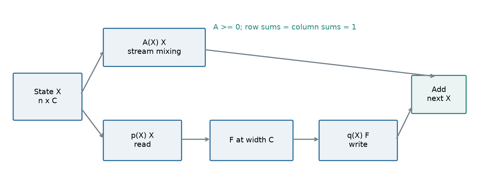
The diagrams and arithmetic examples below are explanatory constructions. The benchmark and ablation charts redraw explicitly tabulated paper values. No model-training results are generated for this review.

2. Prerequisites: streams, norms, and residual paths

For one token, let $X_l\in\mathbb{R}^{n\times C}$ be the state at residual sublayer $l$. A row is a stream; a column is a feature. The expansion factor is $n$, while $C$ remains the width of the expensive function $F_l$. Attention couples tokens elsewhere, but the stream-mixing discussion can be understood with one token at a time. The paper uses $n=4$ in its experiments.

A conventional residual update is $x_{l+1}=x_l+F_l(x_l)$. Unrolling it gives a direct copy of an earlier state plus intervening updates:

$$x_L=x_l+\sum_{i=l}^{L-1}F_i(x_i).$$

This algebra explains the identity route. It does not say that the complete nonlinear network is an isometry, since the update functions can change its derivative substantially. When a paper discusses stability of the shortcut, keep that narrower object separate from stability of the full model.

A matrix norm answers how large an output can become compared with its input. The induced infinity norm is the largest absolute row sum, $\|A\|_\infty=\max_i\sum_j|A_{ij}|$. The induced one-norm is the largest absolute column sum. The spectral norm $\|A\|_2$ is the largest singular value. These quantify different worst-case directions; none alone measures language-model quality.

For nonnegative matrices, row sums and absolute row sums coincide. For signed HC matrices, they need not. The paper describes its Amax statistic in terms of absolute values of row/column sums and visualizes signed mappings. Such a statistic can diagnose large coherent amplification, but cancellation can make it smaller than an induced norm. For example, the row $(10,-9)$ sums to one while its absolute row sum is nineteen. The exact nonnegative mHC argument avoids this ambiguity; the signed HC diagnostic should be interpreted with care.

Two elementary facts will be useful. First, a convex combination uses nonnegative weights that sum to one, so it cannot exceed the scalar range of its inputs. Second, multiplying matrices composes their actions. A modest per-layer gain can therefore become large over depth. A gain of 1.1 repeated sixty times is approximately 304, even before considering the nonlinear branch. This is an illustrative calculation, not a reported HC measurement.

3. What HC changes, and why the shortcut matters

Use $A_l\in\mathbb{R}^{n\times n}$ for residual mixing, $p_l\in\mathbb{R}^{1\times n}$ for reading, and $q_l\in\mathbb{R}^{n\times1}$ for writing. This notation corresponds to the paper’s $\mathcal H^{\mathrm{res}}$, $\mathcal H^{\mathrm{pre}}$, and transposed $\mathcal H^{\mathrm{post}}$:

$$u_l=p_lX_l,\qquad y_l=F_l(u_l),\qquad X_{l+1}=A_lX_l+q_ly_l.$$

The dimensions explain the savings. Reading converts $nC$ stored features into $C$ input features. The large function operates at that width. Writing broadcasts its $C$-dimensional result back into the expanded state using stream-specific coefficients. The architecture increases persistent capacity without making every internal matrix multiplication $n$ times wider.

Let $R_{L:l}=A_{L-1}\cdots A_l$ and define an empty product to be the identity. Unrolling the recurrence gives:

$$X_L=R_{L:l}X_l+\sum_{i=l}^{L-1}R_{L:i+1}q_iF_i(p_iX_i).$$

The multiplication order matters because the matrices do not generally commute. This expression remains an identity along a realized forward trajectory even when coefficients depend on the state. It isolates the direct transport of $X_l$ from later injections. It does not remove the dependence of those injections or matrices on earlier states.

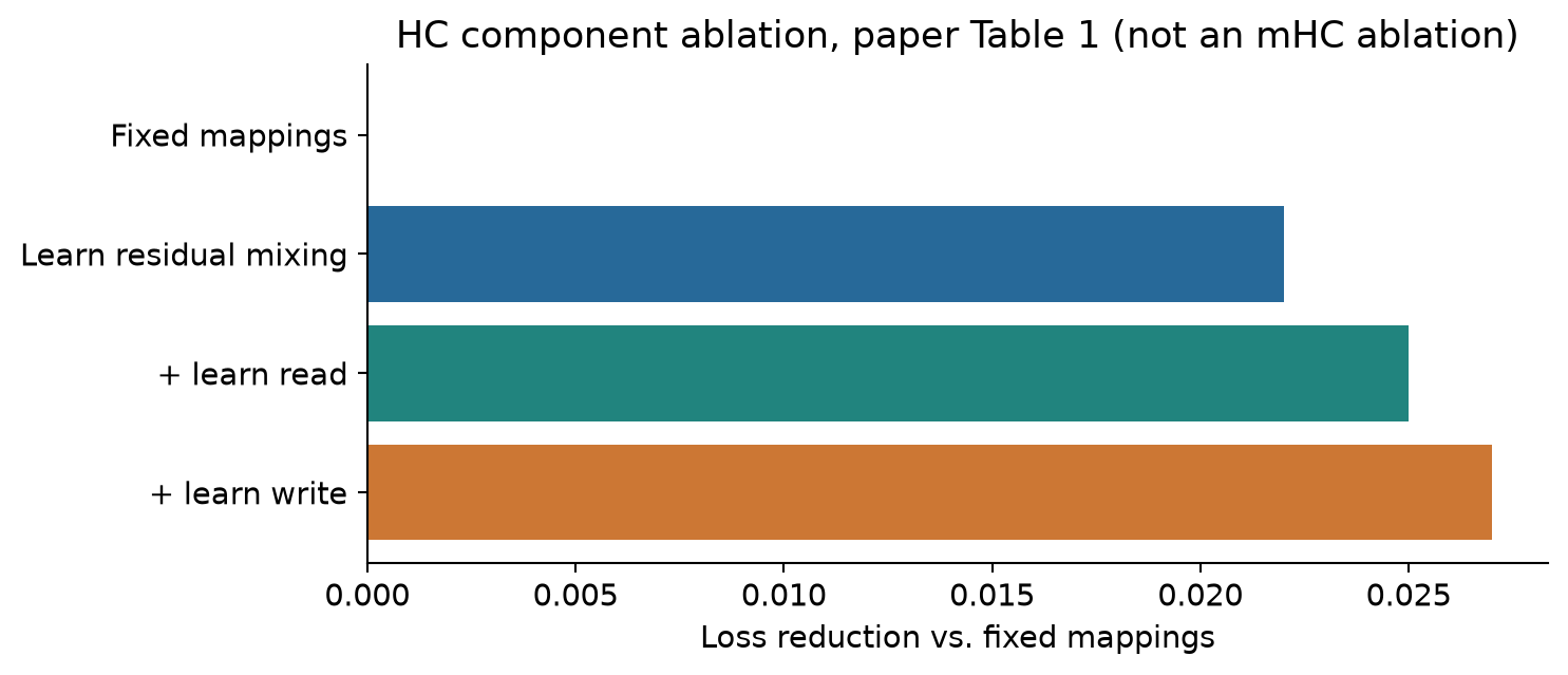
The original HC parameterization combines a static bias with small, input-dependent corrections. mHC keeps the dynamic-plus-static idea but changes the feasible coefficient set. The motivation is supported by paper Table 1: learning only residual mixing produces a loss improvement of 0.022, adding learned reading gives 0.025, and adding learned writing gives 0.027 relative to fixed mappings. These are HC component ablations, not a complete causal decomposition of mHC.

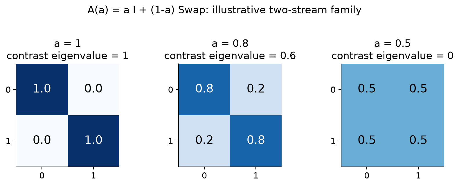
A fixed identity shortcut is the simplest alternative. It has perfect direct transport but prevents learned exchange between the persistent streams through this branch. Unconstrained HC allows richer exchange but lacks a bound on long products. mHC chooses a middle ground: learn mixing inside a restricted nonnegative family. The question is whether that family is expressive enough once the nonlinear branches continue to inject new features.

4. Deriving the doubly stochastic guarantees

Define the feasible set

$$\mathcal B_n=\{A\in\mathbb R^{n\times n}: A_{ij}\ge0,\ A\mathbf1=\mathbf1,\ \mathbf1^TA=\mathbf1^T\}.$$

This is the Birkhoff polytope. Its interior has dimension $(n-1)^2$; the full set includes faces and corners, so the paper’s word “manifold” should not be read as a claim that the entire polytope is a smooth unconstrained surface. The operational object is unambiguous: nonnegative matrices with unit row and column sums.

4.1 Convex averaging and conservation

For feature column $j$, the new value in stream $i$ is $\sum_k A_{ik}X_{kj}$. Row normalization makes this a convex combination. Thus every output lies between the minimum and maximum input value for that feature. Column normalization gives a different property:

$$\bar x'=\frac1n\mathbf1^TAX =\frac1n\mathbf1^TX=\bar x.$$

Row sums control how each destination reads. Column sums control the total weight leaving each source. Only imposing row normalization would not ensure conservation of the mean. For example, a matrix with every row equal to $(1,0,\ldots,0)$ copies the first stream everywhere and discards all other streams.

4.2 Non-expansion in Euclidean norm

For any vector $v$, convexity of the square gives a direct proof:

$$\begin{aligned} \|Av\|_2^2 &=\sum_i\left(\sum_j A_{ij}v_j\right)^2\\ &\le\sum_i\sum_j A_{ij}v_j^2\\ &=\sum_jv_j^2\left(\sum_i A_{ij}\right) =\|v\|_2^2. \end{aligned}$$

The inequality uses the row sums; the final equality uses the column sums. Applying this argument to every feature column yields $\|AX\|_F\le\|X\|_F$. Because $A\mathbf1=\mathbf1$, the largest singular value is actually exactly one for an exact doubly stochastic matrix. Other singular values can be smaller, even zero. “Non-expansion” is consequently more precise than “norm preservation.”

The same conclusion follows from the Birkhoff representation $A=\sum_k\lambda_kP_k$, where $P_k$ are permutation matrices, $\lambda_k\ge0$, and $\sum_k\lambda_k=1$. Each permutation preserves Euclidean norm, and the triangle inequality bounds their convex combination. This interpretation explains why the constraint still allows learned routing: streams can be permuted or blended, although not arbitrarily amplified or subtracted.

4.3 Closure through depth

If $A,B\in\mathcal B_n$, then $AB$ is nonnegative, $AB\mathbf1=A\mathbf1=\mathbf1$, and $\mathbf1^TAB=\mathbf1^TB=\mathbf1^T$. Repeating this reasoning establishes that every finite product is doubly stochastic. It also shows $\|R_{L:l}\|_2\le1$. Transposition preserves the same feasible set, giving the corresponding bound for the frozen linear backward route.

This is a useful depth-independent statement: exact residual transport cannot explode just because many such matrices are multiplied. It is stronger than checking each matrix on a handful of sampled activations. Yet it says nothing positive about the smallest singular value. A stable upper bound on amplification is not a lower bound on information retention.

5. The missing half: what can disappear?

Consider two streams and

$$A(a)=\begin{bmatrix}a&1-a\\1-a&a\end{bmatrix},\qquad0\le a\le1.$$

The mean direction $(1,1)^T$ has eigenvalue one. The contrast direction $(1,-1)^T$ has eigenvalue $2a-1$. Start from $(5,1)^T$, whose mean is three and half-difference is two. With $a=0.9$, after $k$ mixing steps:

$$A(0.9)^k\begin{bmatrix}5\\1\end{bmatrix} =\begin{bmatrix}3+2(0.8)^k\\3-2(0.8)^k\end{bmatrix}.$$

The average survives exactly while the distinction between streams decays. At $a=0.5$, the distinction disappears in one step. At $a=0$, a swap preserves it with alternating sign. All three cases satisfy the same doubly stochastic constraint.

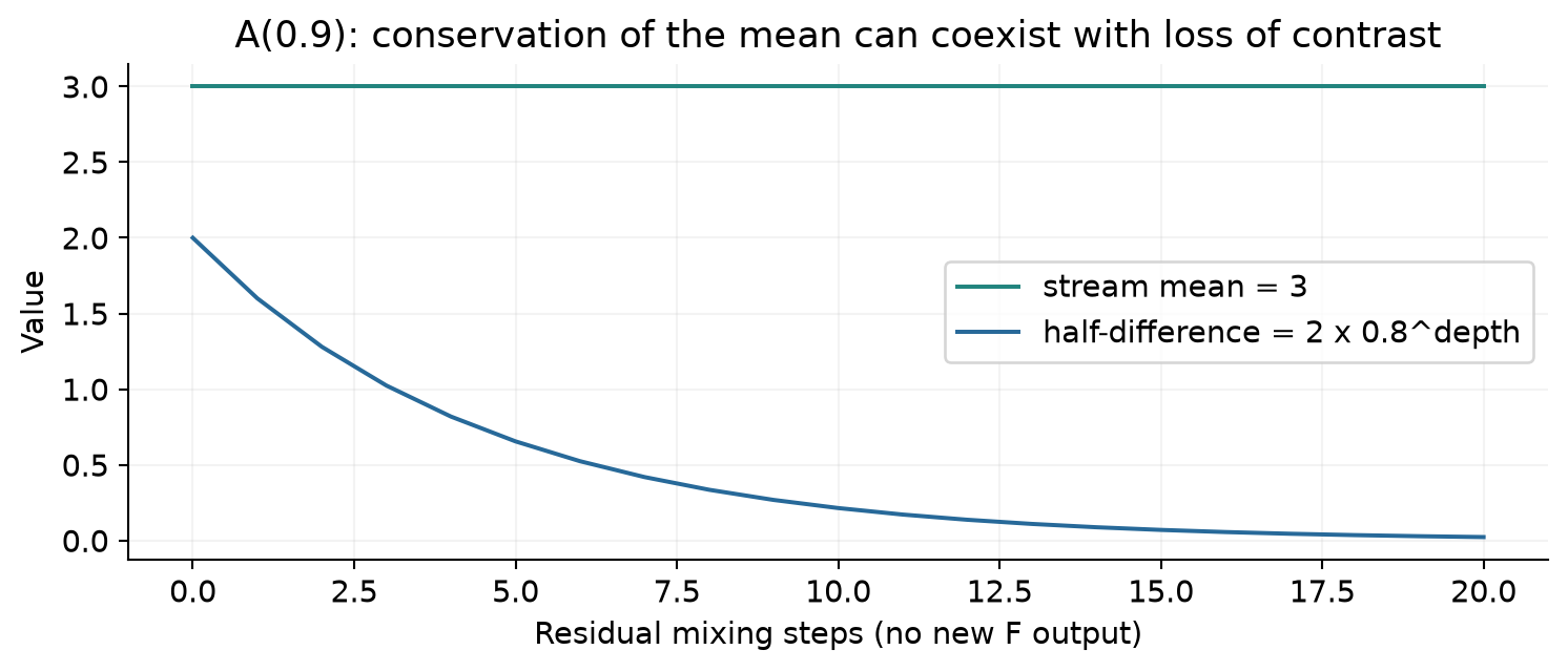
The limiting rank-one map $\mathbf1\mathbf1^T/n$ is perfectly valid and destroys all zero-mean stream directions. Thus exact double stochasticity cannot by itself prevent vanishing gradients in those directions. In the complete model, new features arrive through $q_lF_l$, and data-dependent routing changes from layer to layer, so this counterexample is not evidence that the trained model necessarily collapses. It identifies a behavior the theorem permits and an observable the experiments should measure.

A further subtlety is that consensus need not grow strictly at every layer. A permutation can move streams without mixing them at all. Products of changing matrices can also have behavior that is not summarized by a single eigenvalue. Claims about convergence toward uniform mixing need additional assumptions beyond membership in the polytope. The conservative conclusion is a norm bound and mean conservation for the direct residual route.

6. Parameterization and the actual layer algorithm

mHC computes coefficients from the full flattened state $z_l=\operatorname{vec}(X_l)\in\mathbb R^{1\times nC}$. After RMS normalization, learned projections produce read logits, write logits, and $n^2$ mixer logits. For example,

$$\widetilde A_l=\alpha_l^{\mathrm{res}} \operatorname{mat}(\operatorname{RMSNorm}(z_l)\Phi_l^{\mathrm{res}}) +B_l^{\mathrm{res}}.$$

The read and write formulas have the same structure, with $n$ outputs instead of $n^2$. This full-context parameterization lets a coefficient depend on every stream, not only on the stream that it eventually weights. The projection shapes are $nC\times n$ for each gate and $nC\times n^2$ for mixing. These small output dimensions explain why the extra arithmetic is modest when $n\ll C$, though repeated reads of $nC$ activations remain expensive.

The final maps are

$$p_l=\sigma(\widetilde p_l),\qquad q_l^T=2\sigma(\widetilde q_l),\qquad A_l=\operatorname{SK}(\widetilde A_l).$$

Here SK denotes exponentiation followed by alternating matrix normalization. The read entries lie in $(0,1)$ and the write entries in $(0,2)$ for finite logits. They are not probability vectors: their sums are not constrained to one. Positive coefficients avoid subtraction caused by signed connection weights, but the features being combined can themselves have opposite signs. Nonnegative gates therefore do not eliminate all possible cancellation of activations.

Algorithm 1: One mHC residual sublayer, following paper Eqs. (3), (7)-(9).

1. Receive $X_l$ with shape $n\times C$ and flatten it to $z_l$.
2. RMS-normalize $z_l$; project into $n$, $n$, and $n^2$ coefficient outputs.
3. Apply each learned scalar $\alpha$ and static bias. The reported initial scalar value is 0.01.
4. Apply sigmoid to the read logits and twice sigmoid to the write logits.
5. Apply Algorithm 2 to the mixer logits, using twenty iterations in the reported experiments.
6. Form $u_l=p_lX_l$ and evaluate $y_l=F_l(u_l)$.
7. Produce $X_{l+1}=A_lX_l+q_ly_l$.

This algorithm makes two distinctions explicit. First, the mixing coefficient generator is dynamic, so $A_l$ is not a fixed learned matrix shared by every token. Second, the sublayer function retains its ordinary normalization and computation; normalization used to generate coefficients is a separate operation. Mixing them conceptually would obscure both the math and the activation-memory accounting.

When $n=1$, the mixer is the scalar one. This recovers an identity residual route, as the paper states. It does not automatically make the complete update identical to a conventional residual block, because learned read and write gates can still scale the nonlinear branch. That small distinction matters when designing a clean single-stream control experiment.

7. Sinkhorn normalization: exact limit, approximate execution

Given logits $Z$, begin with the positive matrix $M^{(0)}=\exp(Z)$. Alternately normalize columns and rows. The paper’s Eq. (9) applies column normalization first and row normalization last in each iteration:

$$N_{ij}^{(t)}=\frac{M_{ij}^{(t-1)}}{\sum_k M_{kj}^{(t-1)}},\qquad M_{ij}^{(t)}=\frac{N_{ij}^{(t)}}{\sum_kN_{ik}^{(t)}}.$$

Strict positivity gives the standard convergence setting. At any finite stopping point, the last normalization enforces row sums up to numerical error, while column sums may still deviate from one. Reversing the order exchanges which constraint is exact at the end. That is why a row error near zero does not prove the algorithm has converged.

Algorithm 2: Finite Sinkhorn normalization.

1. Input the $n\times n$ mixer logits $Z$ and iteration count $T$.
2. Set $M=\exp(Z)$; a common scalar shift before exponentiation leaves the exact normalized solution unchanged and can reduce overflow risk.
3. For each iteration $t=1,\ldots,T$, divide each column by its sum.
4. Within the same iteration, divide each row by its sum.
5. Return $A=M$, together with row and column sum residuals if measuring constraint accuracy.
6. Interpret double stochasticity as approximate unless both residuals meet the required tolerance.

The scalar-shift remark is an algebraic numerical consideration, not a claim about the authors’ chosen numerical path. A common shift cannot prevent underflow for arbitrarily separated logits. Very sharp coefficient distributions can slow convergence or worsen finite-precision behavior. A fixed iteration count trades predictable work against an input-dependent approximation error.

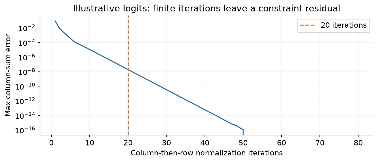
The plot uses rows $(8,1,-1,0)$, $(7,0,1,-2)$, $(0,6,1,-1)$, and $(1,5,-2,0)$. In float64 explanatory arithmetic, the maximum column error after twenty iterations is approximately $1.93\times10^{-8}$. This is deliberately distinguished from the trained-model measurements. The paper reports that twenty iterations leave a composite backward gain as high as approximately 1.6, compared with approximately 3000 for HC in the reported diagnostic. The illustration cannot replace that empirical evidence or imply the same error distribution.

An error budget makes the finite-iteration issue concrete. Suppose $A\ge0$, its row sums equal one, and its maximum column sum is at most $1+\epsilon$. Then

$$\|A\|_2\le\sqrt{\|A\|_1\|A\|_\infty} \le\sqrt{1+\epsilon}.$$

For $K$ such matrices with bounds $\epsilon_l$,

$$\left\|\prod_{l=1}^{K}A_l\right\|_2 \le\prod_{l=1}^{K}\sqrt{1+\epsilon_l} \le\exp\!\left(\frac12\sum_{l=1}^{K}\epsilon_l\right).$$

The final inequality follows from $\log(1+x)\le x$ for $x\ge0$. This worst-case bound is not a prediction of actual gain, because amplifying directions need not align across layers. It does show why one should inspect products or accumulate error budgets instead of treating a small local tolerance as automatically harmless at any depth.

The term “projection” also deserves precision. Sinkhorn rescales a positive matrix into the doubly stochastic set and has an entropy/KL geometry interpretation. It is not generally the nearest matrix under ordinary Euclidean distance. An alternative Euclidean projection would solve a different optimization problem and could yield different sparsity, gradients, and execution costs.

8. Why the full Jacobian remains an open question

For a state-dependent mixer, differentiate $Y(X)=A(X)X$. In a perturbation direction $\Delta X$,

$$DY(X)[\Delta X] =A(X)\Delta X+DA(X)[\Delta X]X.$$

The non-expansion proof controls the first term only. The second term describes the change in routing caused by the perturbation itself. Differentiating the injection $q(X)F(p(X)X)$ adds further terms:

$$\begin{aligned} D[qF(pX)][\Delta X] ={}&Dq[\Delta X]F(pX)\\ &+q\,DF(pX)\left[Dp[\Delta X]X+p\Delta X\right]. \end{aligned}$$

These terms can be large even when every realized $A(X)$ is exactly doubly stochastic. Small initial dynamic scales make the first stages of training less aggressively input-dependent, but learned scales and nonlinear branch derivatives can change later. Thus the paper supplies a controlled transport mechanism and favorable training evidence, not a global Lipschitz theorem for the complete language model.

A useful experimental separation would compare static constrained mixing, dynamic constrained mixing, and dynamic mixing with the coefficient branch detached for a diagnostic derivative calculation. Such a study would distinguish transport effects from routing sensitivity. It would not require assuming the dynamic branch is harmful; that branch may be a substantial source of performance gains. The purpose is to explain which component makes the full optimization behave well.

9. Systems costs: the residual state still has to move

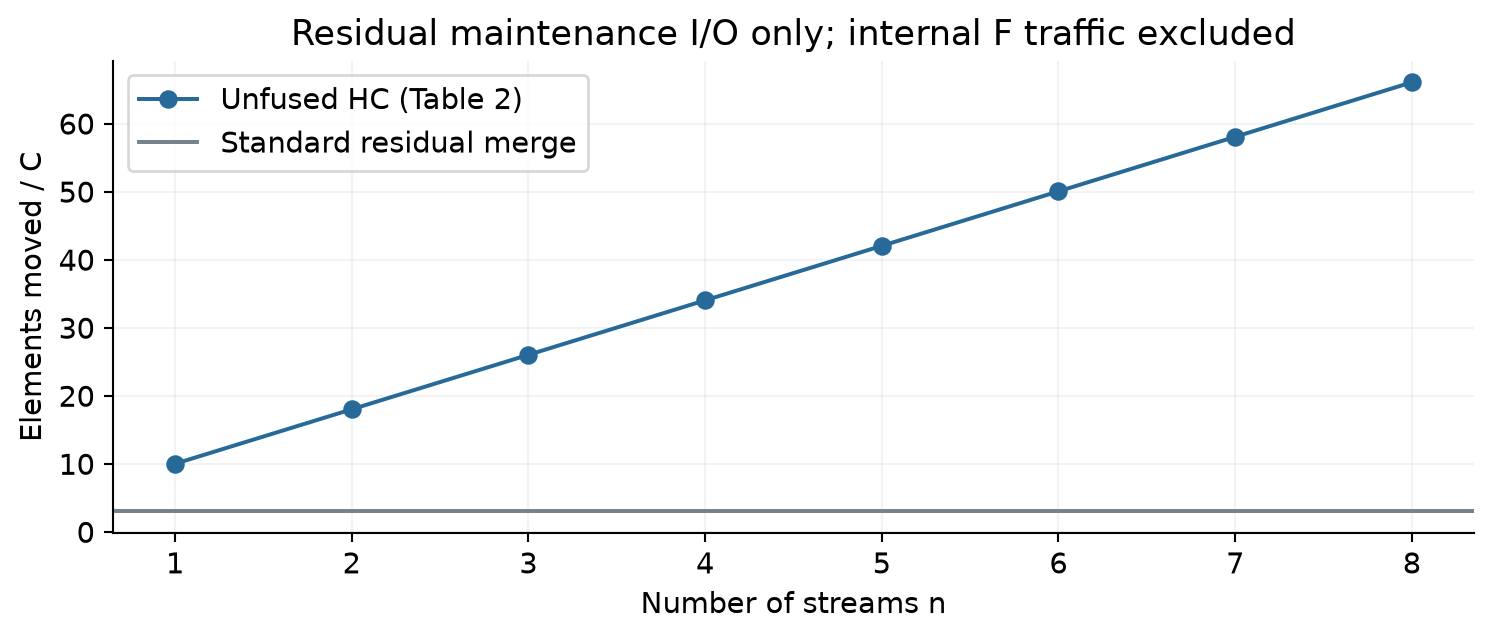
The paper’s Table 2 counts forward memory traffic for residual maintenance, excluding the internal traffic of $F$. A standard merge reads $2C$ elements and writes $C$. For unfused HC, adding the listed operations gives

$$\begin{aligned} R_{\mathrm{HC}}&=(5n+1)C+n^2+2n,\\ W_{\mathrm{HC}}&=(3n+1)C+n^2+2n,\\ R_{\mathrm{HC}}+W_{\mathrm{HC}} &=(8n+2)C+2n^2+4n. \end{aligned}$$

At $n=4$, the leading activation term is $34C$, compared with $3C$ for a standard merge. This ratio, roughly 11.3, is not an end-to-end slowdown prediction. It applies to an unfused subset of operations and says nothing directly about the much larger attention/MLP arithmetic. It explains why counting FLOPs alone gives an incomplete answer.

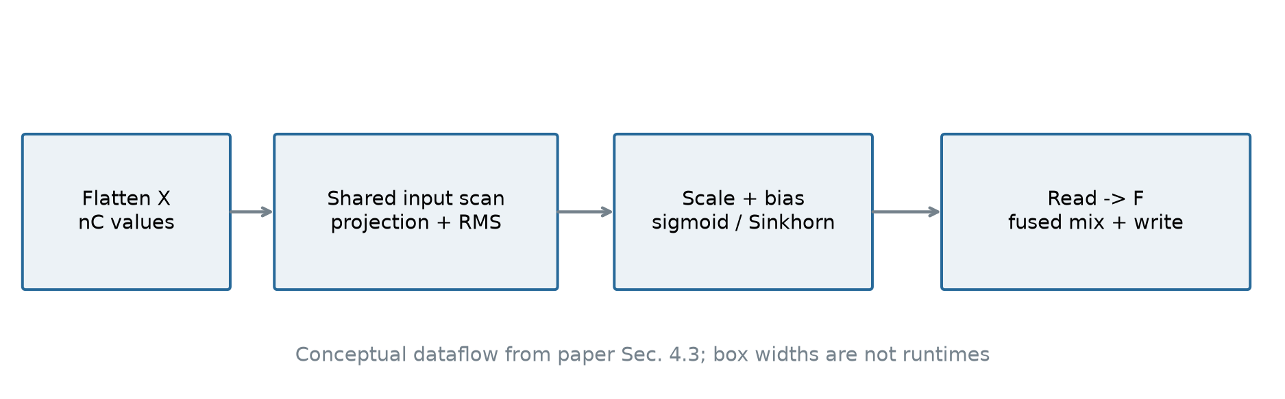
The first optimization moves division by the RMS scale after the small-output projection. If normalized input is $(z\odot\gamma)/r$, then

$$\left(\frac{z\odot\gamma}{r}\right)\Phi =\frac{z\,[\operatorname{diag}(\gamma)\Phi]}{r}.$$

The channel-wise normalization weights can be absorbed into the projection, while the common scalar division applies to the smaller output. This equivalence assumes the same scalar $r$ for the flattened vector; it does not justify rearranging arbitrary nonlinear normalizations. The paper fuses the projection and norm scans, combines lightweight gate operations, and keeps the Sinkhorn iterations in one kernel with recomputation of intermediate states for its backward pass.

The second optimization combines residual mixing, output writing, and addition. The paper reports reducing reads for this combined operation from $(3n+1)C$ to $(n+1)C$, and writes from $3nC$ to $nC$. At $n=4$, this is $25C$ down to $9C$ total elements, a 64% reduction for that particular group. The coefficient-generation and input-reading operations remain, so adding this percentage to an overall speed claim would be incorrect.

Mixed precision is part of this design rather than an incidental detail. Paper Eqs. (10)-(19) identify bfloat16 hidden states, a tfloat32 projection specification, and float32 coefficient-related quantities. The stability of repeated normalizations depends on arithmetic precision as well as iteration count. The paper’s description is sufficient to understand the design tradeoff, but it does not make hardware-independent accuracy or speed guarantees.

10. Recomputing the cheap path and scheduling communication

Saving every expanded state would increase training memory. The proposed strategy keeps the expensive function outputs, stores a wide checkpoint once per group of residual sublayers, and reconstructs intermediate mixing states during backward computation. It does not rerun the heavy function $F$ for this particular recomputation scheme. That distinction is why the design can save memory without proportionally increasing expensive arithmetic.

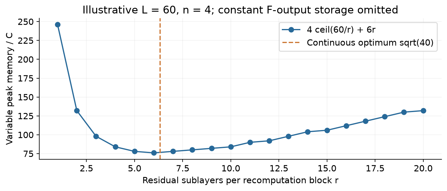
Let a group contain $r$ residual sublayers, with $L$ sublayers in total. Ignoring terms independent of $r$, the paper models peak memory in elements as

$$M(r)=nC\left\lceil\frac Lr\right\rceil+(n+2)Cr.$$

The first term stores wide group-entry states; the second accounts for temporary reconstructed states in the active group. Dropping the ceiling and treating $r$ as continuous gives

$$\frac{dM}{dr}=-\frac{nCL}{r^2}+(n+2)C=0, \qquad r^*=\sqrt{\frac{nL}{n+2}}.$$

The second derivative $2nCL/r^3$ is positive, so this stationary point minimizes the relaxed expression. The derivation does not include all model memory; in particular the per-layer $F$ outputs add storage independent of this choice. Nor does it select the runtime-optimal value when launch overhead, pipeline boundaries, and microbatch concurrency matter.

Algorithm 3: Choosing and using recomputation groups.

1. Count residual sublayers, distinguishing attention and feed-forward sublayers from whole Transformer blocks.
2. Estimate the relaxed optimum from $n$, $L$, and the memory formula.
3. Evaluate nearby legal integer group sizes under pipeline-stage boundaries.
4. During forward computation, retain each group’s entry state and the heavy function outputs needed later.
5. During backward computation, reconstruct the lightweight states for the active group.
6. Release transient states after use and measure the true peak under the actual pipeline schedule.

For the 27B configuration, the appendix lists thirty Transformer blocks, while the stability plots unroll attention and FFN into sixty residual sublayers. Confusing these two conventions introduces a factor-of-two error before any memory calculation begins. The figure’s $L=60$ is an illustrative use of the sublayer convention, not a claim that the authors used groups of six in every pipeline stage.

Pipeline communication exposes a related cost: stage boundaries carry the expanded state. Fusion can remove intermediate GPU reads, but it cannot eliminate the need to convey information required by the next stage. The paper extends DualPipe scheduling, places selected output/mixing work on a high-priority compute stream, avoids long-running persistent attention kernels that would interfere with scheduling, and uses locally cached stage inputs to decouple recomputation from incoming communication.

These measures work only to the extent that useful overlap exists. Faster attention, a slower network, different expert routing, or a smaller microbatch can change which operation dominates. Figure 4 of the paper explicitly uses illustrative block lengths, so its timeline is a dependency explanation rather than a latency measurement. A credible deployment comparison must preserve that distinction.

11. Experiments: what the tables actually establish

11.1 Training configurations

The models are DeepSeek-V3-inspired MoE architectures using MLA, not dense 27B Transformers. Appendix A.1 lists total parameter counts of 2.97B, 9.18B, and 27.0B; the corresponding active parameter entries are 612M, 1.66B, and 4.14B. These entries should retain the appendix’s accounting convention rather than be silently converted into dense-model compute equivalents.

Setting	Blocks	Width	Training tokens	Base learning rate
3B	12	1280	39.3B	$8.6\times10^{-4}$
9B	18	1920	105B	$5.9\times10^{-4}$
27B	30	2560	262B	$4.0\times10^{-4}$
3B long run	12	1280	1.05T	$9.0\times10^{-4}$

All configurations use a sequence length of 4096, expansion factor four, initial dynamic gating scale 0.01, and twenty Sinkhorn iterations for mHC. The appendix specifies AdamW with betas $(0.9,0.95)$, weight decay 0.1, and 2000 warmup steps. The proportional-data runs and the separate long 3B run answer different questions: scaling model/compute together versus continuing token exposure at a fixed model size.

11.2 Downstream evidence

The scores below are transcribed from Table 4. EM means exact match; the DROP score is F1. These are percentage-scale benchmark scores with different evaluation protocols, so their differences are score points, not relative percentage gains.

Task and shots	Baseline	HC	mHC	mHC - HC
BBH, 3	43.8	48.9	51.0	+2.1
DROP, 3	47.0	51.6	53.9	+2.3
GSM8K, 8	46.7	53.2	53.8	+0.6
HellaSwag, 10	73.7	74.3	74.7	+0.4
MATH, 4	22.0	26.4	26.0	-0.4
MMLU, 5	59.0	63.0	63.4	+0.4
PIQA, 0	78.5	79.9	80.5	+0.6
TriviaQA, 5	54.3	56.3	57.6	+1.3

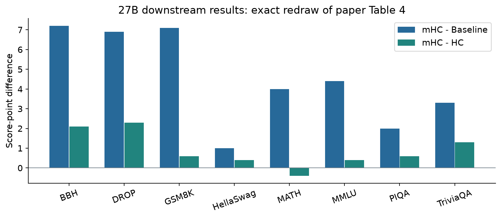
Against the baseline, the gains are 7.2, 6.9, 7.1, 1.0, 4.0, 4.4, 2.0, and 3.3 points in table order. Their unweighted arithmetic average is 4.4875 points, computed here solely as a descriptive summary. It is not a paper-reported aggregate benchmark, and equal weighting does not make tasks equally reliable or equally important. The most persuasive observation is the broad direction of improvement, accompanied by the explicit MATH exception against HC.

11.3 Stability and scaling evidence

Paper Figures 2 and 5 show the HC loss disturbance near step 12,000 and corresponding gradient-norm behavior in the 27B experiment. The mHC trajectory is more stable and finishes 0.021 below the baseline loss. Figure 7 reports approximate conservation along residual mappings, with composite backward gain reaching about 1.6 under finite Sinkhorn iterations. Comparing this with the approximately 3000 HC diagnostic supports a substantial improvement in this measured transport behavior.

However, the plotted matrices and gains are averaged over tokens in a selected sequence. This is not a distribution over all training sequences, nor a full-network Jacobian measurement. An average can conceal outliers, and a sample from one stage of training cannot establish a uniform bound over optimization. The visual evidence is consistent with the mechanism but has a narrower scope than a universal stability guarantee.

The compute-scaling curves span 3B, 9B, and 27B models; the token-scaling curve follows a separate 3B run. They support persistence of the advantage across the reported regimes. They do not provide enough points to establish a new scaling law or a reliable asymptotic crossover. The paper also references in-house large-scale training without exposing comparable detailed configurations for every such run; this review does not infer an undisclosed model size.

12. Limitations of the evidence

Theoretical coverage is narrower than the motivating language. The exact constraint bounds residual transport, yet does not establish invertibility, a lower singular-value bound, or stability of the dynamic coefficient derivatives. Finite Sinkhorn iterations further replace exact feasibility with a measured approximation. These distinctions are especially relevant when moving to deeper networks or sharper learned routing.

The ablation is incomplete for attribution. Table 1 establishes the importance of mixing within HC, but it does not separately attribute the final gain to full-state coefficient generation, nonnegative gates, the factor of two on writing, double stochasticity, and the chosen number of iterations. A row-stochastic control and a static doubly stochastic control would be particularly informative.

The runtime result has a limited portability envelope. The 6.7% overhead is associated with optimized large-scale training. The report does not present a complete hardware-by-model-by-parallelism sensitivity table. A model with cheap internal layers, a network bottleneck, or little overlap opportunity could experience a different overhead. Inference latency and serving memory are separate questions not settled by the training number.

Uncertainty is not quantified by the main benchmark table. Table 4 provides point estimates rather than repeated-seed confidence intervals. Small differences such as 0.4 points should therefore be described as observed differences, without asserting statistical significance. The report also does not establish long-context behavior beyond its listed training length, post-training robustness, or stability across every optimizer configuration.

13. Critical analysis and concrete improvements

13.1 Measure retention alongside amplification

The paper makes a strong case for controlling a dangerous failure mode: explosion along composite residual maps. The next experiment should pair that diagnostic with the nontrivial singular spectrum of those products. Tracking stream covariance, effective rank, and the energy of zero-mean stream components would reveal whether stability is purchased by excessive consensus.

A particularly clean test would freeze the expensive architecture and compare three mixer families: identity, doubly stochastic, and near-permutation doubly stochastic. Holding data, active compute, and tuning budget fixed would help distinguish useful mixing from generic smoothing. If a near-permutation bias improved both retained diversity and downstream performance, the case for managing the lower spectrum would become stronger. If it hurt, the results would indicate that feature blending itself is useful.

13.2 Treat projection accuracy as a measured resource

Twenty iterations are a sensible fixed-work design point, but the paper provides no universal tolerance associated with that choice. A better report would show quantiles of row/column error by layer, token, and training phase, together with rare extremes. It could then compare fixed iteration budgets with a small menu of adaptive budgets chosen from coefficient sharpness or normalization residuals.

Adaptive work is not automatically better. Per-token stopping can cause divergence or scheduling inefficiency on accelerators. A practical alternative is a layer-level or batch-level budget with a small number of discrete choices. The decisive experiment is end-to-end training quality per elapsed time, including any extra reductions used to estimate convergence, rather than normalization accuracy alone.

13.3 Strengthen the causal controls

The complete method changes topology, coefficient generation, constraints, and systems execution together. A factorial study need not explore every possible combination, but it should at least contrast row-only normalization with double normalization, fixed mixing with dynamic mixing, and constrained versus unconstrained read/write gates. The same training recipe and comparable tuning effort should apply to every candidate.

Reporting full-gradient sensitivity separately from frozen-path gain would also sharpen the causal account. The latter can remain controlled while the coefficient generator becomes sensitive. Conversely, the model may learn dynamic routing that improves optimization even though its full derivative lacks a simple worst-case theorem. Measuring both would explain a successful mechanism more convincingly than extending the shortcut guarantee by analogy.

13.4 Price the additional state explicitly

A residual expansion factor is a resource-allocation choice. Compare mHC with spending the same additional wall time or memory on a slightly wider backbone, additional tokens, or a different checkpointing policy. Equal parameter count alone does not price the persistent state, and equal FLOPs does not price communication. Both quality-versus-FLOPs and quality-versus-hours curves are needed.

This comparison should include the point where overlap ceases to hide communication. Record stage-transfer volume, exposed communication time, peak memory, and throughput under several microbatch and pipeline configurations. A system that performs well only when a particular overlap window exists may still be valuable, but its applicability should be stated in those operational terms.

14. A paper-based experimental plan

A future replication should begin by fixing the scientific comparison rather than treating a benchmark score as the entire target. The smallest reported proportional-data configuration provides a starting point: 2.97B total parameters, twelve blocks, width 1280, sequence length 4096, and 39.3B training tokens. This is still a substantial training undertaking, so a smaller pilot could test arithmetic and diagnostics without claiming to reproduce the reported scale.

Algorithm 4: Evaluate the hypothesis with controlled runs.

1. Specify the dataset, tokenization, evaluation prompts, random seeds, model accounting, and training-token budget before comparing architectures.
2. Establish a standard residual baseline and match expensive layer dimensions across HC and mHC.
3. Record coefficient settings, including stream count, gate initialization, normalization iteration count, and arithmetic precision.
4. Measure training loss, full gradient norm, frozen residual-product gains, constraint residuals, and stream-diversity statistics at the same checkpoints.
5. Run downstream evaluations with the exact shot counts and metrics listed in Table 4; retain negative as well as positive task differences.
6. Measure elapsed training time, peak activation memory, and exposed pipeline communication under a documented parallel schedule.
7. Repeat the comparison across seeds or report the uncertainty left by a single run.
8. Compare quality at both equal tokens and equal elapsed budget before drawing a deployment conclusion.

These steps describe a prospective experimental design. The present review performs only source reading, formula derivation, tabulated-value arithmetic, and document checks. The illustrative Sinkhorn and two-stream examples verify mathematical statements in the explanation; they do not replicate the authors’ model training.

The paper appendix is also a useful guard against casual comparisons. It lists a separate 3B long run with a different batch size and learning rate. Combining that loss trajectory with the proportional-data settings as if they were one uninterrupted scaling experiment would erase an important control variable. Likewise, thirty blocks and sixty residual sublayers are two descriptions of the same 27B depth, not two independently reported architectures.

15. Conclusion

mHC is a persuasive example of architectural and systems reasoning meeting at the residual stream. Expanding the persistent state can improve representational flexibility, but stable matrix products and affordable state movement must be designed together. Double stochasticity gives a clear upper bound on exact residual-path amplification and conserves the stream mean. Fusion, recomputation, and scheduling address the costs that FLOP counts miss.

The strongest reading of the evidence is therefore specific: in the reported MoE training settings, constrained mixing improves stability and broad downstream quality at a measured additional runtime cost. The outstanding questions concern retained stream diversity, dynamic routing derivatives, finite normalization error, and portability of the systems result. Those questions make the paper a useful foundation for further work, while keeping its demonstrated gains separate from stronger guarantees that remain unproven.

References and figure provenance

1. Xie et al. mHC: Manifold-Constrained Hyper-Connections, v2. Primary source for the method, experiments, and Appendix A.1. Equation and table references throughout refer to this version.
2. Zhu et al. Hyper-Connections. Contextual antecedent identified in the mHC report; numerical HC results in this review come from mHC’s own comparisons.
3. Sinkhorn and Knopp. Concerning nonnegative matrices and doubly stochastic matrices, Pacific Journal of Mathematics 21(2), 343-348, 1967. Mathematical antecedent cited by the reviewed paper.

Figures 1 and 5 are original explanatory diagrams based on the reported equations and dataflow. Figures 2-4 and 7 are original mathematical illustrations. Figure 6 evaluates the Table 2 traffic expression. Figures 8 and 9 redraw Tables 4 and 1 respectively. No synthetic plot is presented as a model-training observation.