Jacap: Preserving Nonlinear Information in KV-Cache Eviction

Review date: 2026-09-09
Author: Zhongzhu Zhou
Paper reviewed: Jacap: Robust KV Cache Eviction via Jacobian-Based Nonlinear Information Capacity Preservation
Paper authors: Jiaming Yang, Chenwei Tang, Liangli Zhen, Chenyang Zhang, Jiancheng Lv
arXiv: 2609.08131
Venue/Status: Preprint (2026)

1. What problem is the paper solving?

Autoregressive decoding repeatedly attends to every preceding token. To avoid recomputing old hidden states, an inference engine stores a key and value for every layer, attention head, and token. That KV cache grows linearly with context length. At long context or large batch size, capacity is limited by memory before arithmetic throughput is exhausted.

Eviction asks: if only (B) of (N) cached tokens may remain, which ones should survive? Recency, accumulated attention, key norms, and geometric novelty are useful signals, but each is incomplete. They usually rank tokens independently and do not explain how softmax competition changes usefulness.

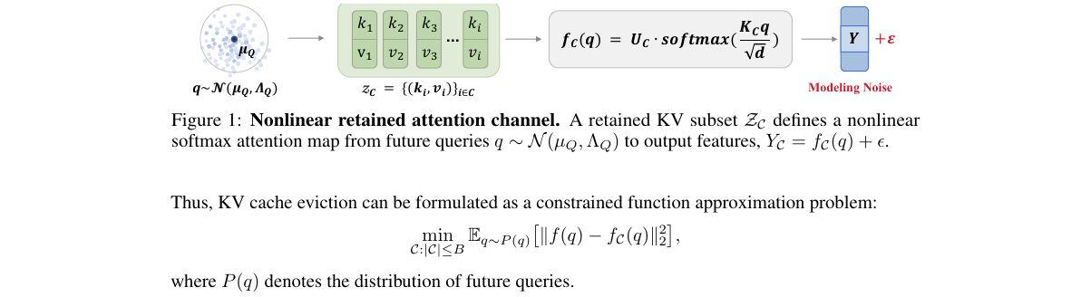
Jacap reframes the cache as a noisy nonlinear communication channel. A future query is the input, retained KV pairs define the channel, and the attention output is the observation. The subset should preserve as much query-dependent information as possible. The paper linearizes attention locally with its Jacobian, derives a Gaussian mutual-information objective, and approximates that expensive objective into an online score.

My verdict: the missing softmax-sensitivity term is real and cleanly derived; results are strongest at aggressive compression. Yet the practical algorithm discards the off-diagonal competition terms that motivate the theory, uses one local query center, and incompletely isolates which approximation causes the gain.

2. Prerequisites: KV caches and attention

For one head at decoding step (t),

$$q_t=W_Qh_t,\qquad k_i=W_Kh_i,\qquad v_i=W_Vh_i,\qquad i\le t.$$

The attention weight and output are

$$\alpha_{t,i} = \frac{\exp(q_t^\top k_i/\sqrt{d_k})} {\sum_{j\le t}\exp(q_t^\top k_j/\sqrt{d_k})}, \qquad o_t=W_O\sum_{i\le t}\alpha_{t,i}v_i.$$

For (L) layers, batch (b), (H_{kv}) KV heads, sequence length (T), head width (d_h), and (s) bytes per scalar,

$$M_{\mathrm{KV}}=2LbH_{kv}Td_hs.$$

Quantization lowers (s); eviction lowers (T). They are complementary.

2.1 Why independent scores are insufficient

If two tokens have nearly identical values, keeping both may double an independent score while adding no new output direction. A moderate-attention token may instead be essential because its value points somewhere absent from the cache. Good eviction must combine:

1. Accessibility: will future queries activate this key?
2. Sensitivity: can a small query change alter its probability?
3. Diversity: does its value add a new output direction?
4. Interaction: does retaining it make another token redundant?

Softmax creates competition: increasing one logit decreases other probabilities because weights sum to one. Attention is not a set of independent channels.

The paper uses compression ratio (c), so the retained count is

$$B=(1-c)N.$$

At (c=0.9), only ten percent remains. Methods can look equal at mild compression yet diverge when one wrong deletion removes unique evidence.

2.2 Future-query statistics

Jacap models

$$q=\mu_Q+\delta q, \qquad \delta q\sim\mathcal N(0,\Lambda_Q).$$

The center (\mu_Q) says where future queries are expected; covariance (\Lambda_Q) says how they vary. A diagonal covariance is practical and makes each key-response variance cheap.

3. Prior art and the missing term

• SnapKV / attention history: cheap and query-aware, but past attention may not predict future use.
• KNorm: large key norm is only a proxy; it ignores query direction and value redundancy.
• KeyDiff: distinct keys need not produce distinct useful outputs.
• Expected Attention: estimates future attention but remains mostly token-wise.
• CapKV: uses linear-Gaussian capacity and leverage scores to capture output diversity.

CapKV assumes

$$Y_C^{\mathrm{lin}}=U_CK_Cq+\epsilon, \qquad \epsilon\sim\mathcal N(0,\Sigma_{\mathrm{noise}}),$$

giving

$$\mathcal L_C^{\mathrm{lin}} = \frac12\log\det \left( I+\Sigma_{\mathrm{noise}}^{-1} U_CK_C\Lambda_QK_C^\top U_C^\top \right).$$

Actual attention inserts softmax between (K_Cq) and (U_C). Normalization saturates dominant tokens and couples every token. Jacap argues that the softmax Jacobian supplies the missing geometry.

4. Nonlinear attention as a local channel

For subset (C), stack keys by row in (K_C) and projected values by column in (U_C), where (u_i=W_Ov_i):

$$f_C(q) = U_C\operatorname{softmax} \left( \frac{K_Cq}{\sqrt{d_k}} \right).$$

Add modeling noise:

$$Y_C=f_C(q)+\epsilon, \qquad \epsilon\sim\mathcal N(0,\Sigma_{\mathrm{noise}}), \qquad q\perp\epsilon.$$

The ideal utility is

$$\mathcal L_C=I(q;Y_C\mid Z_C).$$

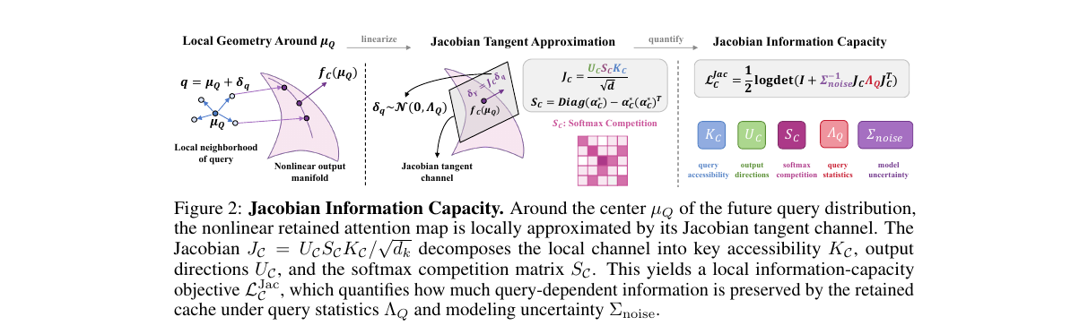
Direct nonlinear mutual information lacks a simple closed form. Let (\delta q=q-\mu_Q). First-order Taylor expansion gives

$$f_C(q) = f_C(\mu_Q)+J_C\delta q +O(\lVert\delta q\rVert_2^2).$$

This tangent approximation is cheap but local; error grows with curvature and distance from the center.

4.1 Deriving the Jacobian step by step

Define

$$z(q)=\frac{K_Cq}{\sqrt{d_k}}, \qquad \alpha(q)=\operatorname{softmax}(z(q)).$$

Since (\alpha_i=e^{z_i}/\sum_j e^{z_j}),

$$\frac{\partial\alpha_i}{\partial z_j} = \alpha_i\left(\mathbf 1[i=j]-\alpha_j\right).$$

Stacking derivatives,

$$\frac{\partial\alpha}{\partial z} = \operatorname{Diag}(\alpha)-\alpha\alpha^\top.$$

Also,

$$\frac{\partial z}{\partial q} = \frac{K_C}{\sqrt{d_k}}.$$

The chain rule evaluated at (\mu_Q) yields

$$J_C = \frac{1}{\sqrt{d_k}}U_CS_CK_C,$$

where

$$S_C = \operatorname{Diag}(\alpha_C^\star) -\alpha_C^\star(\alpha_C^\star)^\top,$$

and

$$\alpha_C^\star = \operatorname{softmax} \left( \frac{K_C\mu_Q}{\sqrt{d_k}} \right).$$

(K_C) maps query perturbations to logits; (S_C) converts logits into coupled probability changes; (U_C) maps those changes into output space.

5. Jacobian information capacity

Under local linearization,

$$Y_C\approx f_C(\mu_Q)+J_C\delta q+\epsilon.$$

The constant bias does not affect mutual information. Conditional and marginal covariance are

$$\Sigma_{Y\mid q}=\Sigma_{\mathrm{noise}},$$ $$\Sigma_Y = J_C\Lambda_QJ_C^\top+\Sigma_{\mathrm{noise}}.$$

For a Gaussian, entropy is

$$h(\mathcal N) = \frac12\log\left((2\pi e)^d\det\Sigma\right).$$

Taking marginal minus conditional entropy cancels the constant:

$$I(q;Y_C\mid Z_C) \approx \frac12 \log \frac{ \det(J_C\Lambda_QJ_C^\top+\Sigma_{\mathrm{noise}}) }{ \det(\Sigma_{\mathrm{noise}}) }.$$

Use (\det(A+B)=\det(A)\det(I+A^{-1}B)):

$$\mathcal L_C^{\mathrm{Jac}} \approx \frac12\log\det \left( I+\Sigma_{\mathrm{noise}}^{-1}J_C\Lambda_QJ_C^\top \right).$$

Substitution gives the paper’s central objective:

$$\mathcal L_C^{\mathrm{Jac}} \approx \frac12\log\det \left( I+ \frac{1}{d_k}\Sigma_{\mathrm{noise}}^{-1} U_CS_CK_C\Lambda_QK_C^\top S_CU_C^\top \right).$$

5.1 Sensitivity, saturation, and competition

Diagonal entries are

$$(S_C)_{ii}=\alpha_i^\star(1-\alpha_i^\star).$$

They vanish as (\alpha_i^\star\to0) or (1), and peak at (1/2). An ignored token and a fully dominant token both have low local sensitivity.

Off-diagonal entries are

$$(S_C)_{ij}=-\alpha_i^\star\alpha_j^\star,\qquad i\ne j.$$

They are negative because increasing one logit suppresses others. The competition matrix also has a useful null-space identity:

$$S_C\mathbf 1=0.$$

This null direction means adding one constant to every logit changes nothing.

For probabilities ((0.5,0.5)),

$$S_C= \begin{bmatrix} 0.25 & -0.25\\ -0.25 & 0.25 \end{bmatrix}.$$

For ((0.99,0.01)), every magnitude falls to (0.0099). High attention is therefore not synonymous with high local information gain.

6. Practical approximation

Exact subset optimization is combinatorial and depends on unknown subset probabilities. Jacap makes four reductions.

6.1 Full-pool attention

Before selection,

$$\bar\alpha_i = \frac{\exp(k_i^\top\mu_Q/(\tau\sqrt{d_k}))} {\sum_{j\in H_t}\exp(k_j^\top\mu_Q/(\tau\sqrt{d_k}))}.$$

This breaks circular dependence, although probabilities will renormalize after eviction.

6.2 Diagonal sensitivity and query response

Replace dense competition by

$$S_C\approx\operatorname{Diag}(\rho_i), \qquad \rho_i=\bar\alpha_i(1-\bar\alpha_i).$$

Replace key-response covariance by

$$K_C\Lambda_QK_C^\top \approx \operatorname{Diag}(\kappa_i), \qquad \kappa_i=k_i^\top\Lambda_Qk_i.$$

Combining them yields

$$w_i = \frac{1}{d_k} \left[\bar\alpha_i(1-\bar\alpha_i)\right]^2 k_i^\top\Lambda_Qk_i.$$

The factors represent center relevance, softmax sensitivity, and variation under likely future queries.

6.3 Capacity matrix and leverage score

With (u_i=W_Ov_i), or (v_i) as a cheaper proxy,

$$A_{\mathrm{Jac}} = I+\sum_{j\in H_t}w_ju_ju_j^\top.$$

Token score is

$$r_i^{\mathrm{Jac}} = w_iu_i^\top A_{\mathrm{Jac}}^{-1}u_i.$$

A direction already represented makes (A_{\mathrm{Jac}}) large there and lowers marginal leverage; a novel direction scores higher.

7. Algorithm 1: one eviction event

Inputs: ({(k_i,v_i)}_{i=1}^N), budget (B), (\mu_Q,\Lambda_Q,\tau).
Output: (C), (|C|=B).

1. Compute (z_i=k_i^\top\mu_Q/(\tau\sqrt{d_k})).
2. Normalize (\bar\alpha=\operatorname{softmax}(z)).
3. Compute (\kappa_i=k_i^\top\Lambda_Qk_i).
4. Compute (w_i=d_k^{-1}[\bar\alpha_i(1-\bar\alpha_i)]^2\kappa_i).
5. Set (u_i=W_Ov_i), or use (v_i).
6. Accumulate (A=I+\sum_iw_iu_iu_i^\top).
7. Factor (A) once; solve (Ax_i=u_i) for every token.
8. Compute (r_i=w_iu_i^\top x_i).
9. Retain the top (B) scores.
10. Reserve mandatory sink/window tokens before filling the flexible budget.

An implementation should use Cholesky solves, not form (A^{-1}), for stability and reuse.

7.1 Why leverage follows from capacity

For a rank-one addition, the determinant lemma gives

$$\det(A+w_iu_iu_i^\top) = \det(A)\left(1+w_iu_i^\top A^{-1}u_i\right).$$

So the log-capacity increment is

$$\Delta_i = \log\left(1+w_iu_i^\top A^{-1}u_i\right).$$

For small increments, (\log(1+x)\approx x), recovering (r_i). Ranking by (x) or (\log(1+x)) is identical for a fixed (A), but Jacap’s one-shot global matrix does not update after each selected token. Sequential greedy selection would better approximate submodular log-determinant maximization but cost more.

7.2 Worked miniature example

Suppose three are three normalized output directions:

$$u_1= \begin{bmatrix}1\\0\end{bmatrix}, \quad u_2= \begin{bmatrix}0.95\\0.05\end{bmatrix}, \quad u_3= \begin{bmatrix}0\\1\end{bmatrix}.$$

Let (w_1=w_2=1) and (w_3=0.7). Independent weighting prefers tokens 1 and 2. Yet they are nearly collinear. The capacity matrix from tokens 1 and 2 has one strong eigenvalue and one weak eigenvalue, while tokens 1 and 3 span both axes. Leverage discounts token 2 because its direction is already covered. This is the structural-diversity contribution that plain attention lacks.

7.3 Complexity and memory

With head width (d_h), diagonal covariance, and (N) candidates:

• logits and weights: (O(Nd_h));
• capacity matrix: (O(Nd_h^2));
• factorization: (O(d_h^3));
• leverage scores: (O(Nd_h^2));
• top-(B): (O(N\log B)) or linear-time selection.

The dominant cost is

$$O(Nd_h^2+d_h^3).$$

Heuristics are usually (O(Nd_h)) or (O(N)). The paper argues (d_h\approx128) and GPU matrix operations make overhead moderate. That can be true for isolated generation, but production serving also pays kernel-launch, synchronization, per-layer invocation, and batching costs.

8. Design choices: why, alternative, boundary

8.1 First-order geometry

Why: it preserves softmax sensitivity and enables closed-form Gaussian capacity.
Alternative: Hessian corrections or Monte Carlo mutual-information estimation.
Boundary: multimodal or rapidly drifting queries may be far from one tangent plane; error scales with curvature and squared displacement.

8.2 Diagonal competition

Why: (\alpha_i(1-\alpha_i)) cheaply retains saturation.
Alternative: keep the exact rank-one correction (-\alpha\alpha^\top), a block approximation, or top-(k) interactions.
Boundary: correlated token groups and normalization effects can be misranked—the discarded term is the explicit competition introduced by the theorem.

8.3 Pre-selection probabilities

Why: full-pool attention resolves dependence on an unknown subset.
Alternative: select greedily and renormalize, or rescore once after a provisional top-(B).
Boundary: at 90% compression, removing competitors can radically change probabilities. Full-pool low-probability tokens may become important after renormalization.

8.4 Values as output proxies

Why: using (v_i) avoids applying (W_O) during eviction.
Alternative: true (u_i=W_Ov_i), a low-rank projected proxy, or residual-stream diversity.
Boundary: (W_O) rotates and mixes head outputs. Diversity before projection need not survive projection.

8.5 Temperature near ten

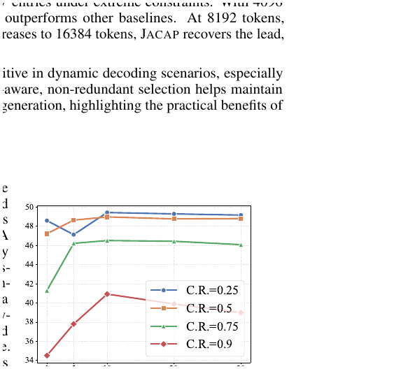
Why: temperature avoids a brittle, excessively sharp center prior. The ablation peaks around (\tau=10).
Alternative: choose (\tau) from attention entropy, layer depth, context length, head role, or compression ratio.
Boundary: one Qwen3-8B LongBench sweep may not transfer across model logit scales.

9. Experimental setup

The evaluation has three complementary views:

1. LongBench: broad long-context quality across single-document QA, multi-document QA, summarization, few-shot learning, synthetic tasks, and code.
2. Needle-in-a-Haystack: sparse retrieval as both context length and needle depth vary.
3. AIME25 online decoding: reasoning while the generated KV cache is dynamically evicted.
4. Runtime: generation of 100 tokens at 8K–64K input lengths and compression ratios 0.6 and 0.8.

Models are Qwen3-8B, Qwen3-14B, Llama-3.1-8B, and Nemotron-7B for AIME25. Baselines include CapKV, SnapKV, Expected Attention, KeyDiff, and KNorm. The appendix reports four RTX Pro 6000 GPUs and Ubuntu 22.04; runtime uses one GPU.

This breadth is valuable: LongBench measures aggregate utility, NIAH exposes location failures, and AIME tests generated-token eviction. But the paper does not report repeated-run uncertainty, memory saved in bytes, throughput under concurrent requests, or end-to-end server tail latency.

10. Results, with quantitative reading

10.1 LongBench

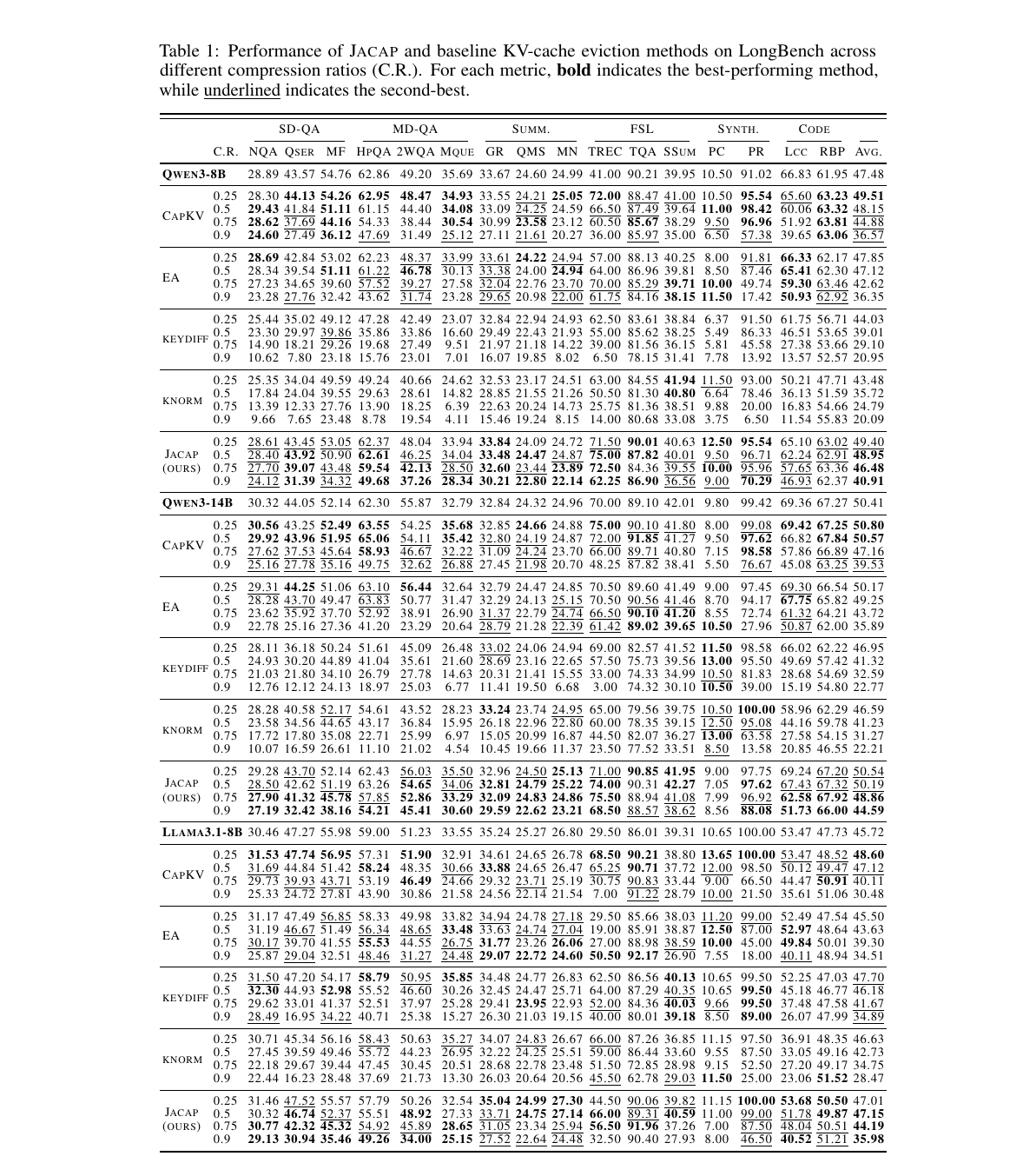
For Qwen3-8B at compression (c=0.75), average scores are Jacap 46.48 and CapKV 44.88. The absolute gain is

$$46.48-44.88=1.60.$$

At (c=0.9), Jacap reaches 40.91 versus CapKV 36.57:

$$40.91-36.57=4.34.$$

This widening gap supports the claim that nonlinear sensitivity matters most when the budget is tight. For Qwen3-14B at (c=0.9), Jacap scores 44.59 and CapKV 39.53, a 5.06-point advantage. On Llama-3.1-8B at (c=0.9), Jacap scores 35.98 versus CapKV 30.48, a 5.50-point gain.

However, “best on average” is not “best everywhere.” At moderate budgets some task columns favor another method, and uncompressed or lightly compressed behavior is already near a ceiling. The evidence supports robust high-compression quality more strongly than universal dominance.

10.2 Needle retrieval

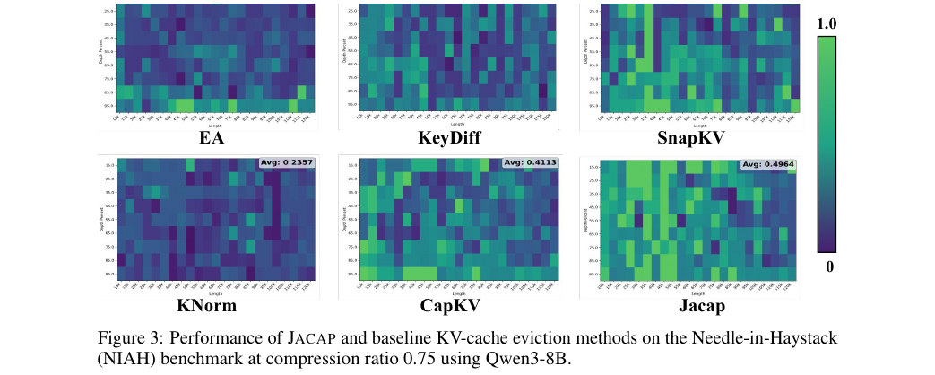
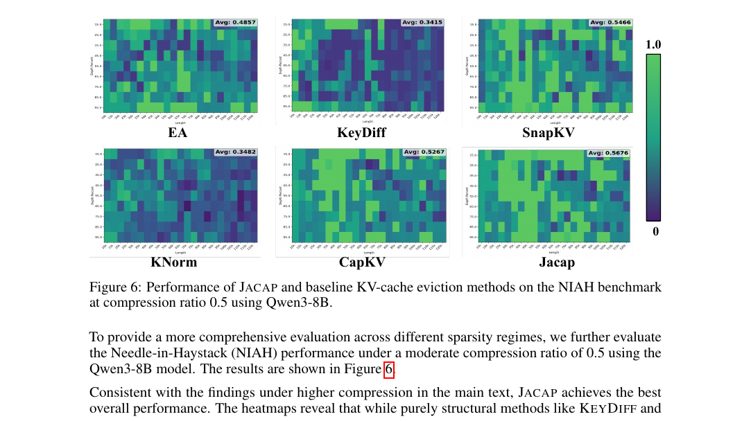
At (c=0.75) on Qwen3-8B, Jacap’s heatmap remains strong over longer contexts and deeper needle positions. KNorm and KeyDiff collapse broadly; attention and CapKV are more competitive but develop holes. This visual benchmark helps because a single average could hide a catastrophic region.

The appendix repeats the comparison at (c=0.5), where Jacap again has the most uniformly successful map.

10.3 Dynamic decoding on AIME25

Reserved-token results for Jacap are 0.30, 0.50, 0.53, and 0.73 at budgets 2048, 4096, 8192, and 16384. CapKV gives 0.20, 0.50, 0.73, and 0.67.

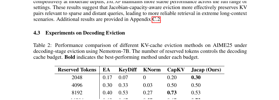
The 8192 reversal is important. It contradicts a monotonic “better theory always wins” story and suggests sensitivity weighting interacts with budget, reasoning phase, or estimation noise. With a small AIME set, score differences may also be only a few problems; confidence intervals are missing.

10.4 Runtime

At 64K context, figure bars place all capacity and heuristic methods in a similar broad range. Jacap does not show prohibitive overhead despite (O(Nd_h^2+d_h^3)) scoring.

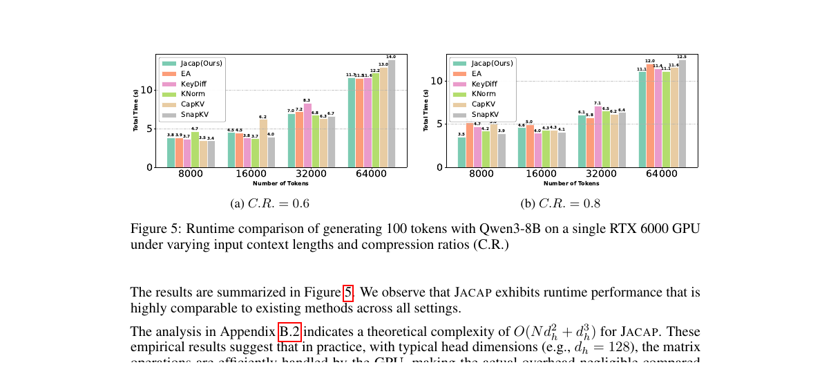
Comparable total time is encouraging, but it is not a complete serving result: prefill/decode separation, peak memory, eviction cadence, batch size, concurrency, and latency percentiles are not reported.

11. Algorithm 2: a serving-safe integration sketch

The paper gives the scoring core, but deployment needs policy around it. A practical control loop is:

1. Initialize per-layer running query mean and diagonal second moment.
2. During decoding, update statistics with an exponential moving average; keep the current request isolated from unrelated tenants.
3. Append new KV entries normally until a high-water mark is reached.
4. Protect mandatory prefix tokens, attention sinks, and a recent sliding window.
5. Run Algorithm 1 only on the remaining candidate region.
6. Fill the flexible budget with highest Jacap scores.
7. Compact or remap physical KV pages without changing logical token positions.
8. Resume decoding and record quality-neutral telemetry: eviction time, retained age distribution, entropy, and memory.
9. Trigger again at a configured interval or high-water mark, not every token.
10. Fall back to a sliding-window policy if factorization fails or exceeds a latency deadline.

The statistics update for mean can be

$$\mu_Q^{(t)} = \beta\mu_Q^{(t-1)}+(1-\beta)q_t,$$

and diagonal second moment

$$m_Q^{(t)} = \beta m_Q^{(t-1)}+(1-\beta)(q_t\odot q_t).$$

Then a nonnegative diagonal covariance estimate is

$$\operatorname{diag}(\Lambda_Q^{(t)}) = \max\left( m_Q^{(t)}-\mu_Q^{(t)}\odot\mu_Q^{(t)},\epsilon \right).$$

The choice of (\beta) is another locality trade-off: high (\beta) is stable but stale; low (\beta) adapts quickly but is noisy.

12. Reproducibility notes

A credible reproduction should fix:

• exact model revisions and tokenizer versions;
• prompt templates and generation parameters;
• which layers and KV heads are compressed;
• whether prompt KV, generated KV, or both are evicted;
• definition of compression ratio and protected tokens;
• update rule for (\mu_Q,\Lambda_Q);
• (\tau), noise scaling, regularization of (A), and numerical precision;
• whether (v_i) or (W_Ov_i) is used;
• eviction cadence and high-water mark;
• task-specific seeds and evaluator versions.

Sanity checks should include:

1. (A) is symmetric positive definite after adding (I).
2. Every (w_i\ge0).
3. Scores are finite under fp16/bfloat16; factorization can remain fp32.
4. Retained count equals budget after protected tokens.
5. Cache remapping preserves RoPE positions and causal semantics.
6. Full-cache mode reproduces the base model.
7. Setting sensitivity to one approximates the CapKV-style structural component.

The paper would be easier to reproduce with released code, explicit query-statistic update details, and a configuration table. The mathematical derivation is more complete than the systems recipe.

13. Limitations and boundary conditions

The authors explicitly acknowledge two approximations: first-order local linearization and token-wise sensitivity in place of pairwise competition. I would add several operational boundaries.

13.1 Query distribution shift

Reasoning traces move through phases: parse, plan, calculate, verify. One center and covariance can average incompatible modes. A token useful for verification may look irrelevant during planning and be evicted before needed.

13.2 Head and layer heterogeneity

Attention heads specialize. Some retrieve delimiters, some copy entities, and some maintain positional or induction patterns. A universal temperature and budget may over-compress rare but critical heads. Layer-level residual mixing also means local head capacity is not identical to end-task utility.

13.3 Softmax saturation is not uselessness

A token with (\alpha_i\approx1) has low local derivative, but deleting it may cause a large discontinuous output change. Jacobian sensitivity measures response to small query perturbations, not leave-one-token-out necessity. Local flatness can coexist with global importance.

13.4 Approximation mismatch after selection

Scores use full-pool attention and a capacity matrix containing all candidates. Once 90% are removed, both normalization and represented output directions change. One-shot leverage is thus evaluated in a geometry that no longer exists.

13.5 Systems cost under load

A single-GPU, one-request runtime plot does not establish throughput under continuous batching. Matrix factorization may serialize with decode kernels or create temporary memory pressure. Eviction can also fragment paged caches and force data movement.

13.6 Evaluation coverage

LongBench and NIAH are useful but aging proxies. They do not cover multi-turn agents, retrieval with distractor semantics, multimodal caches, multilingual long-context generation, or adversarially placed evidence. AIME25 is small enough that several answers alter reported fractions markedly.

14. Critical analysis

14.1 Paper-specific weaknesses and flaws

First, the theory’s signature interaction is removed. The paper motivates Jacap with the dense off-diagonal matrix (-\alpha\alpha^\top), then the algorithm diagonalizes it. The empirical method proves that a squared sensitivity weight plus leverage works; it does not prove that preserving nonlinear competition caused the gain.

Second, ablations are too narrow. The visible ablation varies only temperature. Needed factorial ablations include: CapKV plus sensitivity; sensitivity without leverage; full versus diagonal query covariance; (v_i) versus (W_Ov_i); static versus adaptive query statistics; and one-shot versus rescored selection.

Third, statistical reporting is weak. There are no confidence intervals, repeated seeds, paired significance tests, or NIAH aggregate summaries. AIME fractions particularly need exact counts and uncertainty.

Fourth, notation and implementation linkage are incomplete. The theory contains (\Sigma_{\mathrm{noise}}), but practical scaling is absorbed into weights. The estimator for (\mu_Q,\Lambda_Q), regularization, cadence, and protected-token policy are insufficiently specified for faithful reproduction.

14.2 Limitations understated or omitted

1. Low derivative versus deletion damage: the objective can penalize saturated tokens even when removing a dominant token radically changes output.
2. RoPE and position dependence: future query-key geometry depends on relative positions; a stationary Gaussian query prior may not capture phase rotation over long long horizons.
3. Group-query attention: shared KV heads serve multiple query heads with distinct distributions. Aggregating their statistics may erase minority-head needs.
4. Cache causality: once a token is evicted, later query statistics are generated from a changed model trajectory. The selection policy changes its own future input distribution.
5. Security and reliability: an adversarial prompt may manipulate attention sensitivity to force retention of distractors or eviction of policy-critical content.
6. Energy and temporary memory: headline cache savings can be partly offset by scoring buffers and repeated matrix construction.
7. Calibration across layers: logit scales and entropy vary by layer; fixed (\tau) makes sensitivity incomparable without normalization.

14.3 Concrete improvements

Preserve the rank-one competition correction. Because

$$S=\operatorname{Diag}(\alpha)-\alpha\alpha^\top,$$

the omitted part is structured, not arbitrary dense noise. Derive efficient products (Sx) without materializing (S), and test whether low-rank-aware scores improve difficult budgets.

Use mixture-local query models. Maintain (K) centers and diagonal covariances, assign the current query to a mode, and aggregate worst-case or weighted capacity. This covers planning-to-verification shifts better than one Gaussian.

Rescore after provisional selection. A two-pass method can compute top-(2B), renormalize within that set, rebuild capacity, and select (B). It costs more than one-shot scoring but directly reduces selection-geometry mismatch.

Protect globally important saturated tokens. Blend local sensitivity with a leave-one-out or historical-attention floor:

$$\tilde w_i = \lambda w_i^{\mathrm{Jac}} + (1-\lambda)g_i^{\mathrm{global}}.$$

This guards against confusing local flatness with dispensability.

Allocate budgets per head and layer. Optimize a global memory budget using measured marginal quality or capacity, instead of assigning identical ratios everywhere.

Strengthen evaluation. Add LongBench-v2 or similarly difficult tasks, multi-turn agent traces, retrieval with semantic distractors, batch serving throughput, p50/p99 latency, peak temporary memory, quality-memory Pareto curves, and at least three seeds.

Release a minimal fused implementation. A Triton/CUDA kernel that forms weighted Gram matrices and batched Cholesky solves would make the systems claim testable.

15. What I would measure next

A useful diagnostic separates three errors:

$$E_{\mathrm{total}} \le E_{\mathrm{Taylor}} + E_{\mathrm{diagonal}} + E_{\mathrm{selection}}.$$

Measure (E_{\mathrm{Taylor}}) by comparing actual attention-output changes with (J_C\delta q). Measure (E_{\mathrm{diagonal}}) by comparing full and diagonal Jacobian covariance on sampled subsets. Measure (E_{\mathrm{selection}}) by comparing one-shot top-(B) with iterative greedy selection on small caches where exact search is feasible.

This decomposition would turn “nonlinear capacity helps” into a falsifiable account of where accuracy is gained and lost.

16. Practical takeaways

For an inference engineer, the paper suggests a useful hierarchy:

1. Preserve protected prefixes and a recent window for safety.
2. Estimate likely future-query directions rather than use key norm alone.
3. Include softmax saturation; raw high attention is not always high marginal information.
4. Include output diversity; independent importance duplicates capacity.
5. Use stable factorization and batch head-sized matrix operations.
6. Validate end-to-end latency, not only algorithmic complexity.
7. Under distribution shift, prefer guarded hybrid scores over pure local geometry.

For a researcher, the most interesting result is conceptual: KV eviction can be studied as local information geometry. The Jacobian links attention mechanics to capacity in an interpretable chain. The most important open question is whether a tractable method can retain the competition structure rather than only its diagonal.

17. Conclusion

Jacap advances KV-cache eviction from empirical ranking toward a mechanistic objective. Starting with nonlinear softmax attention, it derives

$$J_C = \frac{1}{\sqrt{d_k}}U_CS_CK_C$$

and the local capacity

$$\mathcal L_C^{\mathrm{Jac}} \approx \frac12\log\det \left( I+\Sigma_{\mathrm{noise}}^{-1}J_C\Lambda_QJ_C^\top \right).$$

Its practical score combines query variability, softmax sensitivity, and leverage-based output diversity. Across three model families, LongBench gains become largest at 90% compression; NIAH heatmaps remain robust; AIME25 shows both wins and an instructive middle-budget loss; runtime appears comparable in the tested single-GPU setup.

The paper is strongest as a derivation and high-compression empirical result. It is weaker as proof that the full nonlinear-competition story survives approximation, and as a production serving evaluation. A low-rank competition correction, multimodal query statistics, two-pass rescoring, and stronger ablations are concrete next steps.

18. Compact derivation map

The complete reasoning chain is:

1. Retained attention is nonlinear: (f_C(q)=U_C\operatorname{softmax}(K_Cq/\sqrt{d_k})).
2. Linearize around (\mu_Q): (f_C(q)\approx f_C(\mu_Q)+J_C\delta q).
3. Chain rule introduces (S_C=\operatorname{Diag}(\alpha)-\alpha\alpha^\top).
4. Gaussian perturbation plus noise yields a log-determinant capacity.
5. Diagonalize sensitivity and query response into token weights (w_i).
6. Build (A=I+\sum_iw_iu_iu_i^\top).
7. Use leverage (w_iu_i^\top A^{-1}u_i) to reward marginal output diversity.
8. Keep top (B), while recognizing renormalization and locality boundaries.

This map is also the checklist for reproducing—or challenging—the method.