Strong Drafts Need Compact Memories: A Technical Review of Memory-Augmented Sliding-Window (MASW) Drafting for Long-Context Speculative Decoding

Review date: 2026-09-06 Paper reviewed: Strong Drafts Need Compact Memories: Long-Context Speculative Decoding with Compressed KV Cache Paper authors: Tong Yuan, Chengxi Liao, Zeyi Wen (HKUST Guangzhou) arXiv: 2608.30252 Venue/Status: EMNLP 2026 Findings

1. What Problem Is This Paper Actually Solving?

Long-context LLM applications — document summarization, multi-turn agents, “deep research” style tool use — routinely condition generation on prefixes spanning tens of thousands of tokens. Autoregressive decoding is already slow because it is memory-bandwidth-bound: each new token requires streaming every model weight and the entire KV cache from GPU HBM. Speculative decoding (SD) tries to fix this by having a cheap draft model propose several tokens, then verifying them all in a single parallel forward pass through the target model. The catch this paper identifies is a genuine dilemma that nobody had cleanly resolved before: SD’s speedup depends on two things pulling in opposite directions as the prefix grows.

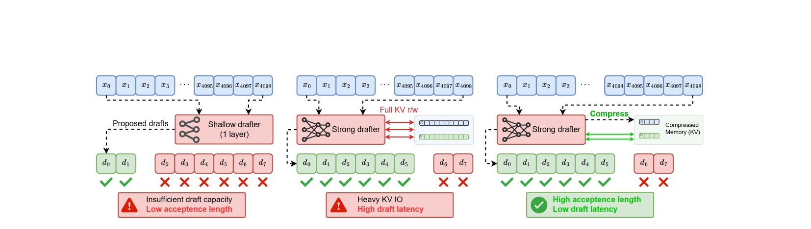
A lightweight draft (the EAGLE family: a single shallow autoregressive layer bolted onto the target) is cheap per step, but its capacity to approximate the target model’s true distribution degrades as context grows — it simply doesn’t have the parameters to track long-range dependencies, so its accepted-token count collapses at long context (the paper’s own Figure 3a shows EAGLE’s accepted length falling from about 2.1 to under 1.0 as context grows from 1K to 32K tokens). A strong, independent draft (e.g., a separate 3B or 8B model) keeps its acceptance length high regardless of context length, because it has enough capacity to genuinely track the distribution — but it pays the price of streaming its own full KV cache at every draft step, and that KV-access cost grows linearly with prefix length, eventually dominating and eroding the very speedup SD was supposed to deliver.

The paper’s contribution, Memory-Augmented Sliding-Window (MASW) Drafting, is a way to get both properties at once: keep a strong, independent draft model’s approximation quality (and thus its high acceptance length), but replace its full historical KV cache with a small, fixed-shape compressed working memory — a sink-token prefix, an exact recent local window, and a chain of periodically materialized “memory slots” that a lightweight trainable adaptor produces to summarize everything older than the local window. The target model’s verifier is completely untouched: it keeps its full, uncompressed KV cache and applies the standard speculative accept/reject rule, so the lossless correctness guarantee of SD is preserved exactly — only the draft side changes. Measured on Llama 3.1-8B and 70B targets at prefixes up to 32K tokens, MASW cuts draft-side memory by over 70% and delivers speedups up to 2.08x (8B target) and 3.33x (70B target) over plain autoregressive decoding, while EAGLE, EAGLE-3, sliding-window attention, and SnapKV baselines all lose speedup (sometimes falling below 1.0x, i.e. slower than no speculation at all) as the prefix grows past 16-24K tokens.

2. Prerequisites: What You Need to Understand First

2.1 Autoregressive decoding and its memory-bandwidth bottleneck

A transformer LLM generates text one token at a time: run a forward pass, sample the next token, append it, repeat. Each forward pass at generation time is memory-bandwidth-bound rather than compute-bound — producing one new token requires reading every model weight, plus every entry currently sitting in the KV cache, from GPU HBM into on-chip memory, while the GPU’s arithmetic units mostly sit idle. This idle-compute gap is exactly what speculative decoding is designed to exploit: if a single forward pass over the target model can verify several candidate tokens at once instead of just one, you get proportionally more useful output per weight-read.

2.2 Speculative decoding, formally

Given a target model $M_t$ and a cheaper draft model $M_d$, one SD iteration runs $M_d$ autoregressively for $L_{\text{draft}}$ steps to propose a candidate continuation, then invokes $M_t$ once, in parallel, over all $L_{\text{draft}}$ candidate positions to compute what the target’s own distribution would have produced at each position. Let $L_{\text{acc}}$ denote the mean number of accepted draft tokens per iteration (accepted meaning: matches what rejection sampling against the target distribution would have produced); ignoring early termination, the mean number of tokens emitted per iteration is $L_{\text{emit}} = L_{\text{acc}} + 1$ (the accepted tokens, plus either a correction token after the first rejection, or a bonus token if everything was accepted). Let $t_d$ and $t_t$ be the single-token latencies of the draft and target models respectively. The decoding speedup over plain autoregressive decoding is:

$$\text{Speedup} = \frac{L_{\text{acc}} + 1}{L_{\text{draft}} \cdot \frac{t_d}{t_t} + 1}. \tag{1}$$

It is worth unpacking why this formula has exactly this shape. The numerator counts how many tokens you get “for the price of” the denominator’s cost. The denominator has two pieces: $L_{\text{draft}} \cdot t_d/t_t$ is the total draft-side wall-clock cost (across all $L_{\text{draft}}$ sequential draft steps), expressed as a multiple of one target-model forward pass; the trailing $+1$ is the cost of the single target verification pass itself, normalized to 1 (since $t_t$ is the unit here). So the whole expression is “tokens emitted” divided by “total wall-clock cost expressed in units of one target forward pass” — a genuinely dimensionless speedup ratio. Two competing levers are visible immediately: raising $L_{\text{acc}}$ (a stronger, more target-faithful draft) helps the numerator; lowering $t_d/t_t$ (a cheaper, faster draft relative to the target) shrinks the denominator. The paper’s entire argument is that these two levers are normally in tension — a stronger draft (higher $L_{\text{acc}}$) tends to be a slower draft (higher $t_d$), and MASW’s job is to decouple them.

2.3 KV cache attention, and why it’s what makes both draft and target slower as context grows

For an ordinary softmax-attention layer, decoding step $t$ needs a key/value cache $K, V \in \mathbb{R}^{T \times d}$ built from every one of the $T$ prior tokens:

$$\text{Attn}(q_t, K_{\le t}, V_{\le t}) = \text{softmax}\!\left(\frac{q_t K_{\le t}^\top}{\sqrt{d}}\right) V_{\le t}. \tag{2}$$

Decomposing single-token decode latency into a fixed weight-loading term and a KV-access term that scales with prefix length $L$:

$$T_{\text{decode}} \approx \alpha d^2 + \beta L d, \tag{3}$$

where $d$ is hidden size. The first term ($\alpha d^2$) is fixed per backbone — loading the model’s own weights from HBM — and does not depend on context length at all. The second term ($\beta L d$) is what actually grows: streaming the historical KV cache means reading $O(L \cdot d)$ floats from HBM per decode step, and this dominates once $L$ gets into the thousands of tokens. The paper’s own empirical decomposition (its Figure 3b) confirms this directly: per-token decode latency for a fixed model scales almost linearly in prefix length, and the slope of that line — not the intercept — is what differs across model sizes. This is the mechanistic reason a strong independent draft model, which is itself a real transformer with its own growing KV cache, becomes slow at long context in exactly the same way the target model would: it is paying the same $\beta L d$ tax, just with a smaller $d$.

2.4 Why the two existing draft strategies each fail at long context (the dilemma, made precise)

Eq. (1) says a draft needs to be simultaneously target-faithful (high $L_{\text{acc}}$) and cheap (low $t_d/t_t$). EAGLE-style methods — a single lightweight autoregressive layer bolted onto the target’s own hidden states — satisfy both at short context: the layer is cheap, and it is accurate enough over a short history to approximate the target well. But its capacity is fixed and shallow, so as the prefix grows into the tens of thousands of tokens, its ability to track long-range dependencies degrades, and $L_{\text{acc}}$ collapses (the paper’s Figure 3a shows this directly, alongside a genuinely independent 3B draft model whose $L_{\text{acc}}$ stays flat across the same range). The independent-draft alternative fixes the capacity problem but reintroduces the KV-access problem of §2.3: because it is a full transformer conditioning on the full historical prefix, its own decode latency grows linearly with $L$ via Eq. (3), exactly like the target, just with smaller constants. Neither strategy alone satisfies both terms of Eq. (1) at long context — this is the design gap MASW is built to close.

3. Method: Memory-Augmented Sliding-Window (MASW) Drafting

3.1 From full-KV drafting to a three-part compact working memory

The starting point is that a pure sliding window (retaining only the most recent $W$ tokens’ exact KV, discarding everything older) is the simplest possible fix for the KV-access cost, but it is too crude: discarding all information beyond the window frontier misaligns the draft’s conditioning with the target model’s true full-prefix conditional distribution, which directly hurts acceptance length. MASW’s design choice is to augment the window rather than replace it outright, with a third component — learned memory slots — that carries forward a compressed summary of everything the window has already evicted.

Formally, at decoding step $t$, the draft’s entire working memory is a union of three disjoint pieces:

$$\mathcal{M}_t = \mathcal{M}_{\text{sink}} \cup \mathcal{M}_{\text{local}, t} \cup \mathcal{M}_{\text{slot}, t}. \tag{4}$$

• $\mathcal{M}_{\text{sink}}$: the exact raw KV of the first $S$ tokens of the sequence (the “sink” set $\mathcal{S} = \{1, \ldots, S\}$), following the sink-plus-local-window structure introduced by StreamingLLM. These stay resident throughout prefill and decoding and are never evicted. Sink tokens are known empirically (from the StreamingLLM line of work) to anchor attention distributions even when their semantic content is otherwise unremarkable — dropping them causes a disproportionate accuracy collapse relative to their small count.
• $\mathcal{M}_{\text{local}, t}$: the exact raw KV of the most recent $W$ non-sink tokens — $\mathcal{M}_{\text{local}, t} = \{(K_i, V_i) \mid \max(S{+}1, t{-}W{+}1) \le i \le t\}$. This is the part that preserves precise, uncompressed recent context, which matters because immediately-preceding tokens tend to carry the highest-precision signal for next-token prediction.
• $\mathcal{M}_{\text{slot}, t}$: the accumulated set of memory slots — compact, dense, fixed-shape KV entries produced by a trainable adaptor, one materialized for every $r$ raw tokens that fall outside sink and local window (the design in §3.2 below).

Because the draft only ever touches $S$ sink entries, $W$ local entries, and $\lfloor t/r \rfloor$ memory slots, its working-set size scales with these three small, bounded quantities — never with the full prefix length $t$ itself. This is the structural reason MASW’s per-step draft latency stays flat as context grows, unlike a full-KV independent draft whose working set (and hence its $t_d$ in Eq. 1) grows linearly with $t$.

3.2 Memory materialization: how a slot is actually produced

Algorithm 1 — Memory-slot materialization (unpacked from the paper’s Eq. 5-6 into explicit numbered steps)

Input: current draft-side memory M_t = (M_sink, M_local,t, M_slot,<m) at
       compression boundary tau_m = m*r (i.e. every r raw tokens, excluding
       sink tokens), frozen draft backbone f_theta with additional trainable
       mirrored projection parameters
Output: a new memory slot g_m appended to M_slot

1. At boundary tau_m, insert a special memory-slot token position g_m into
   the token stream, immediately following the r-th raw token since the
   last boundary.
2. Run g_m through every one of the draft backbone's transformer layers
   under a STRUCTURED attention mask (Appendix C of the paper): g_m may
   attend to M_local,tau_m (the current local window about to be evicted),
   M_sink, and M_slot,<m (all previously materialized slots) -- but NOT to
   ordinary raw tokens outside those sets.
       g_m <- f_theta(M_local,tau_m, M_sink, M_slot,<m)
3. At every transformer layer l, compute g_m's key/value using DEDICATED
   "mirrored" projection matrices W_K,g^(l), W_V,g^(l) that are separate
   from (and initialized as a copy of, then fine-tuned away from) the
   backbone's ordinary raw-token projections W_K,r^(l), W_V,r^(l):
       K_g^(l) = H_g^(l-1) W_K,g^(l),   V_g^(l) = H_g^(l-1) W_V,g^(l)
   Ordinary raw-token KV continues to use the original (frozen) W_K,r^(l),
   W_V,r^(l) -- only the mirrored matrices are trainable.
4. Append (K_g^(l), V_g^(l)) for every layer l to M_slot,t.
5. Evict the raw KV of tokens now outside the retained local window --
   their information is no longer stored verbatim, but remains accessible
   downstream only through g_m's compressed KV.
6. Assign g_m the SAME RoPE position ID as the raw token immediately
   following it (a deliberate duplicate ID, not a shifted one -- this keeps
   subsequent raw-token position IDs unperturbed by slot insertion).
7. Repeat at every subsequent boundary tau_{m+1} = (m+1)*r as decoding
   proceeds; each new slot's forward pass can read all EARLIER slots
   (M_slot,<m), so slots form an incremental compression CHAIN, not
   independent disjoint summaries.

The key design intuition behind step 2-3 is captured by the paper’s phrase “structured attention as write policy”: rather than hand-designing a pooling rule (e.g., averaging evicted tokens’ KV, or some fixed compression formula), the training objective itself — ordinary next-token prediction loss, computed over raw tokens conditioned on the compressed memory $\mathcal{D}_t = (\mathcal{M}_{\text{sink}}, \mathcal{M}_{\text{local},t}, \mathcal{M}_{\text{slot},t})$:

$$\mathcal{L} = \sum_t -\log p(x_t \mid \mathcal{D}_t, x_{<t}), \tag{5}$$

— forces each slot to become whatever representation functionally replaces the evicted raw tokens for the purpose of predicting future tokens, because that is literally the only signal the gradient carries. Memory-slot positions are themselves excluded from the loss (they aren’t prediction targets), so the slot’s entire “job,” as learned, is compression-for-future-prediction rather than summarization-for-its-own-sake or exact reconstruction of individual evicted KV entries.

Why mirrored (not shared) projections — the design choice, unpacked. Using dedicated $W_{K,g}^{(l)}, W_{V,g}^{(l)}$ rather than reusing the backbone’s own $W_{K,r}^{(l)}, W_{V,r}^{(l)}$ decouples two things that would otherwise be conflated: the information-aggregation computation happening inside the slot’s hidden state $H_g^{(l-1)}$ (which flows through the same shared transformer blocks as everything else) from the KV entries the slot actually writes into the cache (which get their own projection). The obvious alternative — just reuse the raw-token projections for slot tokens too — would force the slot’s KV representation to live in exactly the same subspace as ordinary token KV, even though a slot’s job (compress $r$ tokens’ worth of information) is qualitatively different from an ordinary token’s job (represent one token). The paper’s ablation (§3.4, Figure 6 below) shows this design choice matters concretely at the initialization level: whether the mirrored matrices are initialized as an exact copy of the backbone’s pretrained KV projections, or randomly, produces a large and persistent training-loss gap — random initialization never catches up to copy-initialization even after 300 pretraining steps. This is strong indirect evidence that the subspace the mirrored projections start in genuinely matters, not just that they are trainable.

Where this design still costs something. Only the mirrored projection parameters are trainable; the frozen backbone (including its ordinary raw-token projections) is entirely untouched, which keeps training cheap but caps how much the adaptor alone can reshape what information a slot can retain — the paper’s own Limitations section flags that jointly fine-tuning a larger subset of draft parameters (e.g. MLP blocks, or low-rank updates on the backbone) is a natural but unexplored extension that might raise the ceiling on how much each slot can encode.

3.3 Speculative decoding integrated with MASW: prefill and rollback

Algorithm 2 — Full MASW speculative-decoding loop (unpacked into explicit steps)

PREFILL:
1. Target model M_t prefills the full prefix, building its complete,
   unmodified full KV cache (unchanged from standard SD).
2. Draft model M_d (independent backbone) processes the SAME prefix in
   ONE forward pass, using the structured memory-write mask of Appendix C,
   to construct its initial compressed memory M_0 = (M_sink, M_local,0,
   M_slot,0) -- memory slots ARE materialized during this single prefill
   pass, not deferred to decoding.
3. Because the draft is an independent model, its prefill can run
   CONCURRENTLY with the target's prefill (they don't depend on each
   other's KV). Actual wall-clock prefill time is
       T_prefill^MASW = max(P_d, P_t) = P_t   (since P_d < P_t empirically)
   i.e. the (larger) draft-side prefill cost is HIDDEN behind the
   (larger) target prefill and adds zero to time-to-first-token in this
   regime.

DECODING (per speculative iteration):
4. Draft model M_d autoregressively proposes L_draft candidate tokens,
   reading only its compact M_t (sink + local + slots) at every step --
   NOT the full historical prefix.
5. Target model M_t verifies all L_draft candidates in one parallel
   forward pass over its OWN full, uncompressed KV cache -- standard
   accept/reject rejection sampling per Eq. (1)'s SD framework, UNCHANGED
   by any draft-side compression. This is what preserves the lossless
   guarantee.
6. IF the target accepts a prefix of length L_acc < L_draft (rejects at
   least one candidate):
     - Discard the draft's speculative local KV and any memory slots
       materialized strictly after the last accepted position (ROLLBACK).
     - The retained raw-KV rollback window (16 tokens in the paper's main
       config) recovers the draft's active local context after rejection,
       without needing to recompute a full earlier state from scratch.
7. Advance to the next speculative iteration with the (possibly rolled
   back) M_t, repeating steps 4-6.

The one non-obvious design detail worth dwelling on is why concurrent prefill (step 3) is a real win rather than an accounting trick: because the draft and target are independent models with no shared KV, there is no dependency forcing the draft’s prefill to wait for the target’s, so running them on separate compute streams genuinely overlaps their latency rather than merely reordering it. This only pays off, of course, because the draft’s own prefill (even with memory materialization overhead) is empirically faster than the target’s (§5.3’s Table 2 confirms: even an 8B draft with memory materialization prefills faster than a 70B target at every tested prefix length up to 32K) — if the draft were ever slower to prefill than the target, this concurrency benefit would disappear and TTFT would grow.

The obvious alternative, and why the paper rejects it. One might ask: why not skip the sliding window and sink tokens entirely, and let the draft rely purely on memory slots, materializing one every token? The paper’s window-size ablation (§3.4) answers this indirectly — accepted length is not monotonic in local-window size, peaking at $W=128$ and decreasing again at $W=256, 512$ — suggesting that too little exact local context (window too small) loses acceptance from imprecise recent-token representation, while too much (window too large, in the tested range) does not straightforwardly help either, likely because it dilutes how often slots get materialized relative to how much the local window itself can already cover. The three-part design (sink + local + slots), rather than either extreme, is the configuration the paper’s own sweep finds best.

4. Implementation and Experiment Setup

Models and hardware. Target models: Llama 3.1-8B-Instruct and Llama 3.1-70B-Instruct. Independent draft backbones: Llama 3.2-3B-Instruct and Llama 3.1-8B-Instruct (i.e., an 8B model can itself be paired as a draft for the 70B target). MASW equips each draft backbone with the mirrored-projection memory adaptor described in §3.2; the draft backbone stays entirely frozen and only the adaptor parameters are trained. All inference measurements run on a single 8xH100 (80GB) node at batch size 1. MASW configuration: local-window width and sink-token count are both set to $W = S = 128$ (so every memory slot observes the same number of visible raw tokens by construction); a 16-token raw-KV rollback window is used for post-rejection recovery; separate adaptors are trained for nominal $4\times$ and $8\times$ compression ratios (i.e., $r=4$ and $r=8$ raw tokens per materialized slot, roughly).

Training. Two-stage recipe: continued pretraining on 2B tokens sampled from RedPajama (general web-scale text, each document delimited by an end-of-sequence token), followed by supervised fine-tuning (SFT) on task-oriented long-context data drawn from LongAlpaca and BookSum, all sequences truncated to 8K tokens. The training objective is exactly Eq. (5) above: next-token prediction loss over raw tokens conditioned on the compressed draft memory, with memory-slot positions themselves excluded from the loss.

Datasets. Mixed long-input summarization tasks from LongBench-v1: GovReport, QMSum, and MultiNews — all chosen specifically because they require attending to information distributed across the entire prefix rather than concentrated near the boundaries, which is exactly the regime where a naive sliding window (with no memory slots) would be expected to fail.

Baselines, four categories: (1) vanilla autoregressive (AR) decoding; (2) standard SD with an uncompressed full-KV draft; (3) EAGLE and EAGLE-3, the leading short-context SD methods (single lightweight autoregressive layer on the target); (4) component-level draft-side KV-reduction baselines using sliding-window attention (SWA, 1,024-token window) and SnapKV (4,096 retained KV entries, official default configuration).

Metrics. Tok./Iter (mean tokens emitted per speculative iteration — this is exactly $L_{\text{emit}}$ from Eq. 1, not applicable to AR decoding), decoding throughput (tok/s, output tokens divided by decoding wall-clock time, excluding prefill), and Speedup over the AR baseline under matched prefix length. All speculative methods propose 5 draft tokens per iteration in the main comparison (a separate motivation experiment, Figure 3a, uses a 10-token horizon specifically to make EAGLE’s degradation more visible).

5. Results & Analysis

5.1 Main results: MASW is the only method that doesn’t decay with context length

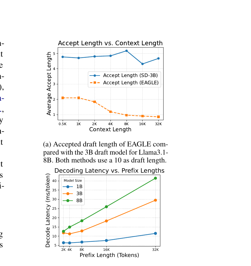
Table 1 (reproduced below) sweeps two target scales (8B, 70B) across four prefix lengths (8K, 16K, 24K, 32K). The qualitative story is consistent across both scales: EAGLE and EAGLE-3 provide little or inconsistent acceleration at long context (EAGLE actually drops to 0.59x at 16K on the 8B target — slower than plain autoregressive decoding), confirming the capacity-collapse mechanism of §2.4. SWA is the most fragile baseline of all, falling to 0.37-0.52x speedup range at long context on the 8B target, because discarding all distant KV (no memory slots to compensate) sharply reduces accepted length. Full-KV SD (an uncompressed independent draft) also loses speedup as the prefix grows, because its own draft-side KV traffic grows with context exactly as Eq. (3) predicts — it starts competitive (1.16-1.18x at 8K) but degrades toward parity (0.91-0.98x) by 24-32K. MASW is the only family of methods whose speedup does not decay with context length; its strongest configurations (Ours 8x L8B on the 8B target, Ours 4x L8B on the 70B target) reach up to 2.08x and up to 3.33x speedup respectively, and — notably — these are the highest speedup values in the entire table at the longest tested context (32K for the 8B target; 16K for the 70B target), i.e. MASW’s relative advantage over every baseline grows rather than shrinks as context lengthens, which is the opposite direction from every other method in the table.

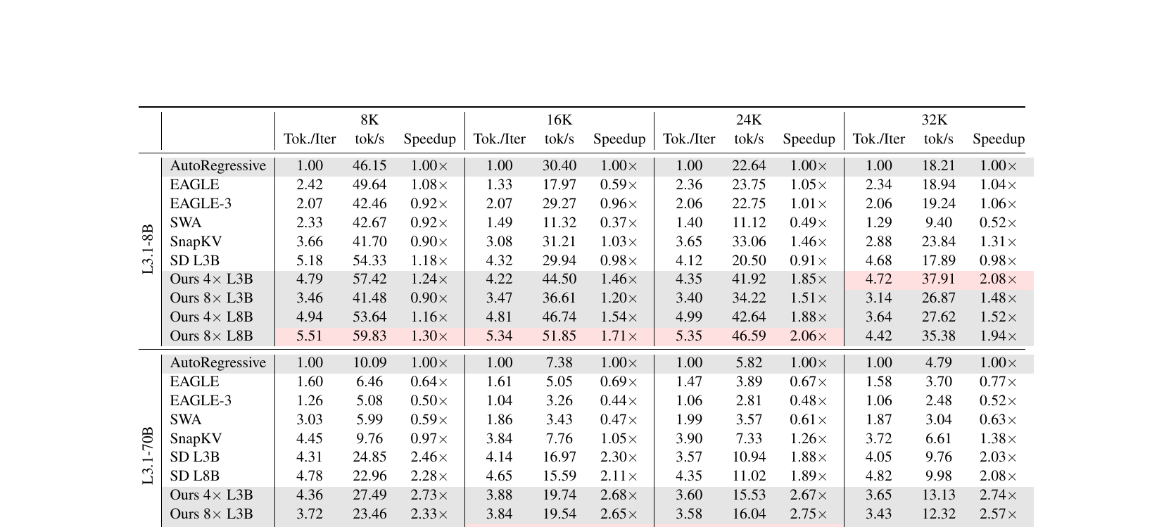
Across the eight MASW variants shown (2 draft backbones x 2 compression ratios x 2 targets), a clear pattern emerges: 4x compression tends to preserve more tokens per iteration (higher Tok./Iter, i.e. closer to full-KV acceptance quality) at the cost of somewhat higher draft latency, whereas 8x compression further reduces draft latency at some cost to Tok./Iter — making the best compression ratio a function of target scale and prefix length rather than a single universally-best setting. Concretely, at 32K on the 8B target, “Ours 4x L3B” achieves the single best speedup (2.08x) with Tok./Iter of 4.72, while “Ours 8x L3B” trades some Tok./Iter (3.14) for a smaller model of savings that doesn’t pay off as well at this particular scale — showing the ratio choice genuinely interacts with target scale rather than being dominated by one setting throughout.

5.2 Draft-side efficiency: where the memory and latency actually go

The paper’s Table 3 (32K prefix, Llama 3.1-70B target) makes the memory story concrete: a 3B draft’s extra peak GPU memory (beyond backbone weights — the KV cache, attention masks, logits, and temporary buffers) drops from 17.21 GB (full-KV) to 4.42 GB (MASW 4x) or 3.98 GB (MASW 8x) — over a 70% reduction — while Tok./Iter falls only modestly, from 4.05 to 3.65 (4x) or 3.43 (8x). The corresponding draft-latency picture is even more dramatic: 41.34 ms (full-KV) collapses to 13.94 ms (4x) or 12.39 ms (8x) — roughly a 3x latency reduction for a Tok./Iter cost of well under 20%. The 8B draft tells the same qualitative story at slightly higher absolute numbers (18.02 GB -> 4.55-5.05 GB extra peak; 54.92 ms -> 14.02-15.37 ms latency; Tok./Iter 4.82 -> 3.77-3.78). This is the concrete numerical evidence behind the paper’s headline “>70% memory reduction” claim, and it shows the memory and latency savings are not merely correlated with a small acceptance-quality hit — they substantially outpace it (a roughly 3-4x resource reduction for a roughly 10-20% Tok./Iter reduction).

Prefill latency, worked through numerically. Table 2 shows the 8B draft’s own prefill latency actually increases substantially when equipped with memory materialization (306.5ms -> 751.6ms at 8K prefix; 1835.2ms -> 7992.5ms at 32K — roughly a 4-4.5x increase, since materializing memory slots during prefill is itself extra computation over the raw prefill forward pass). Naively, this looks like a regression. But because this cost is hidden behind the target’s own (much larger) prefill latency — 2212.9ms at 8K, 12316.4ms at 32K for the 70B target, always larger than even the memory-augmented 8B draft’s prefill time at every tested length — Eq. (4)‘s concurrent-prefill scheduling means this extra draft-side cost adds zero wall-clock time to time-to-first-token in this configuration. This is a good illustration of why the paper reports both the raw draft-prefill cost (which looks bad in isolation) and the scheduling argument for why it doesn’t matter in the end-to-end pipeline (which it does not, provided the draft stays faster than the target, an assumption that could break down for larger drafts or smaller targets than tested here).

5.3 Ablation study: four design choices, unpacked with why/alternative/boundary

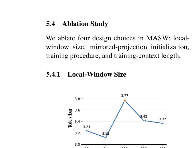
(a) Local-window size (§5.4.1). Sweeping $W=S \in \{32, 64, 128, 256, 512\}$ (with $S=W$ held equal so every slot observes the same local context) at nominal 8x compression on the 70B target at 32K prefix, Tok./Iter is not monotonic: it rises from 3.24 (W=32) to a peak of 3.77 (W=128), then falls back to 3.42 (W=256) and 3.37 (W=512). Why this shape, not simply “bigger window is always better”: a too-small window loses acceptance because too little exact recent context is retained verbatim (the local window is where precision matters most, per §3.1); a too-large window, in the tested range, appears to not help further and even hurts slightly — plausibly because a larger window means fewer materialization boundaries relative to the same total context, giving the memory-slot mechanism fewer opportunities to actually exercise its compression pathway during training and evaluation, though the paper does not give a mechanistic explanation for the exact decline beyond reporting the empirical peak. The alternative (always use the largest window that fits) is directly contradicted by this ablation. The boundary: this sweep is run at one specific compression ratio, target scale, and prefix length; whether 128 is the universally-best window size across all configurations, or an artifact of this specific setup, is not established.

(b) Mirrored projection initialization (§5.4.2). Copy-weight initialization (mirrored $W_{*,g}^{(l)}$ start as an exact copy of the backbone’s own pretrained $W_{*,r}^{(l)}$) versus random initialization, both pretraining the 3B adaptor at nominal 4x compression. Figure 6/Figure 7 (right) shows a large, persistent gap: random initialization starts at roughly 3.5x the loss of copy-weight initialization and never catches up even after 300 pretraining steps; the gradient-norm trace tells the same story — random-init stays elevated and noisy throughout training, while copy-init decays into a small, stable regime within tens of steps. Why this matters: preserving the backbone’s own KV geometry at initialization gives the optimizer a strong starting point that a from-scratch random projection has to rediscover the hard way, and apparently doesn’t fully rediscover even after hundreds of steps under this training budget. The alternative (random init, simpler to implement, no dependency on backbone weight structure) is the one the paper explicitly tested and rejected based on this evidence. The boundary: this is tested on the 3B adaptor at one compression ratio (4x) with a fixed 300-step budget — it’s plausible random init would eventually converge given a much larger training budget, but the paper doesn’t test this, so “never catches up” should be read as “never catches up within this budget,” not as a permanent ceiling.

(c) Training recipe (§5.4.3). Three recipes compared at 16K context across both draft backbones (3B, 8B) and both compression ratios (4x, 8x): pretraining (PT) alone, SFT alone, and the full two-stage PT+SFT pipeline. PT+SFT wins in every one of the four (backbone x ratio) cells, e.g. 4.15 vs. 3.70 (PT-only) vs. 3.23 (SFT-only) for the 3B/4x cell, and the advantage of the two-stage recipe over PT-alone widens under 8x compression (4.78 vs. 3.78 for 3B/8x, a bigger gap than the 4x case’s 4.15 vs. 3.70) — consistent with the paper’s interpretation that when the adaptor must compress more information into fewer slots, the extra alignment SFT provides (matching the memory slots to the actual downstream drafting distribution, not just to general next-token prediction) matters proportionally more. The alternative (SFT alone, skipping pretraining) is consistently the worst of the three recipes across every cell, suggesting supervised data alone cannot teach the adaptor robust general-purpose compressed representations — it needs the broader pretraining signal first. The boundary: this recipe comparison is run at one context length (16K); whether the PT+SFT advantage holds, widens, or narrows at 32K is not directly tested in this ablation (though the main results in §5.1 use the full recipe throughout, so its efficacy at 32K is implicitly confirmed there, just not isolated against the other two recipes at that length).

(d) Training-context length (§5.4.4). Training the 8B adaptor at nominal 8x compression using either 8K-token or 32K-token training sequences (fixed 2B-token total training budget either way), then evaluating both against the 70B target across 8K-32K contexts. The 8K-trained adaptor wins at every evaluated length, including 32K itself (3.77 vs. 3.58 at 32K) — i.e., training on the shorter sequence length generalizes better to the longer evaluation length than training directly on the matching long length does. Why: under a fixed token budget, 8K sequences yield more distinct training instances than 32K sequences do (more documents seen, each shorter), and because MASW’s slot-materialization operation is relative (each slot combines a bounded local window, sink tokens, and earlier slots — an operation with no absolute-position dependence), this relative operation generalizes across context lengths the way, say, RoPE’s relative position encoding generalizes, rather than requiring training data that matches the eventual absolute deployment length. The alternative (train directly at the target evaluation length, the “obvious” choice if one assumed length-matching mattered) is directly falsified by this result. The boundary: this is one specific training-budget/context-length pairing (2B tokens either way); it isn’t established whether an even larger training budget would eventually favor long-sequence training, or whether this data-efficiency argument holds at context lengths far beyond the tested 32K ceiling.

3.4 A worked numerical walk-through of one materialization boundary

It helps to trace through Algorithm 1 with concrete numbers rather than only symbols. Suppose $W=S=128$ and $r=4$ (nominal 4x compression), and decoding has just reached global position $t=4100$, i.e. exactly at a compression boundary $\tau_m = 4100$. Immediately before materialization, the draft’s working memory (Eq. 4) holds: the sink set $\mathcal{M}_{\text{sink}} = \{s_1, \ldots, s_{128}\}$ (positions 1-128, always resident); a chain of previously materialized slots $\mathcal{M}_{\text{slot}, <m} = \{g_4, g_8, g_{12}, \ldots, g_{4088}, g_{4092}\}$ — one slot for every 4 raw tokens processed since the sink, i.e. $(4092 - 128)/4 \approx 991$ slots so far; and the exact local window $\mathcal{M}_{\text{local}, 4100} = \{x_{4092}, \ldots, x_{4099}\}$ (the 8 most recent raw tokens). At this boundary, the draft inserts slot token $g_{4100}$, which attends (per the structured mask of Algorithm 1, step 2) to exactly these three sets — sink, all earlier slots, and the current local window — and nothing else. Its mirrored-projection KV pair $(K_{g_{4100}}^{(l)}, V_{g_{4100}}^{(l)})$ is computed at every layer $l$ and appended to $\mathcal{M}_{\text{slot}, t}$. The raw tokens $x_{4092}, \ldots, x_{4096}$ (those now more than $W=128$… — actually those falling outside the next local window) are evicted once the window advances past them; their information is no longer stored as raw KV, but remains reachable only through $g_{4100}$ and the slot chain behind it. The crucial accounting point: the draft’s total working-set size at this instant is $128 \text{ (sink)} + 8 \text{ (local)} + 991 \text{ (slots)} = 1127$ slot-equivalent entries — versus a full-KV draft’s $4100$ raw entries at the same position — already a roughly $3.6\times$ reduction at this relatively early position, and the ratio keeps improving as $t$ grows further, because sink and local stay fixed size while the raw prefix that a full-KV draft would need to store keeps growing linearly.

6. Limitations & Boundary Conditions

What the authors state explicitly. (1) Training resources are limited to 2B tokens at an 8K training context, leaving open a broader study of adaptor-training configurations — longer training contexts, larger training corpora, and full fine-tuning of the draft model (rather than just the mirrored K/V projections) so it could learn context compression more natively. (2) Training only the mirrored K/V projections keeps the adaptor lightweight but may cap how much information each slot can encode; jointly fine-tuning a larger subset of draft parameters (MLP blocks, or low-rank updates on the backbone) is explicitly flagged as a natural but unexplored extension. (3) MASW currently fixes the local-window size, sink-token count, and slot interval to obtain regular masks, stable cache layouts, and bounded materialization overhead — the paper explicitly notes adaptive allocation of these quantities (e.g., varying slot density based on content, rather than a fixed period $r$) remains future work. (4) The paper explicitly notes MASW “could also compress the draft path in self-speculative decoding” (where the draft is a shallow exit from the target itself, rather than a fully independent model) but flags that using the target model or part of it for long-context drafting may weaken cost-effectiveness, and leaves this trade-off to future work.

What the paper does not fully spell out, but a careful reader should notice. First, all reported speedups are measured at batch size 1 on a single 8xH100 node — production serving systems typically run at much higher concurrency where the target model’s own verification pass is competing for GPU compute across many concurrent sequences, and it is not established whether MASW’s per-sequence draft-latency reduction translates proportionally into system-level throughput gains once the target-side verification (not the draft) becomes the shared bottleneck resource across many requests. Second, the ablations in §5.3 are each run at one specific (backbone, ratio, target, prefix-length) configuration rather than a full factorial sweep — the window-size ablation, for instance, uses only the 70B target at 32K with the 8B draft at 8x compression, so whether $W=128$ remains optimal for the 3B draft, for 4x compression, or at other prefix lengths, is inferred rather than directly demonstrated. Third, the rollback mechanism (§3.3, retaining a 16-token raw-KV window to recover context after a rejection) is described but its own cost — how often rejections occur in practice, and whether frequent rejections near a compression boundary could force expensive re-materialization of slots — is not separately quantified; the main throughput numbers presumably already reflect this cost since they’re measured end-to-end, but the paper doesn’t isolate “rollback overhead” as its own line item the way it does for prefill latency (Table 2) or memory (Table 3).

7. Critical Analysis

(a) Weaknesses and flaws specific to this paper. First, every ablation in §5.3/§5.4 of the paper is a single-point sweep (one backbone, one ratio, one target, one prefix length varied at a time) rather than a factorial design — this makes it genuinely hard to know whether the reported optimal settings ($W=S=128$; copy-weight init; PT+SFT; 8K training context) are robust defaults across the full configuration space the main results table (Table 1) actually sweeps, or whether they happen to be tuned to whichever single configuration each ablation used, with untested interaction effects lurking (e.g., does the optimal window size shift for the 3B vs 8B draft, or for 4x vs 8x compression?). Second, the paper reports Tok./Iter and throughput as its primary metrics throughout, but never reports downstream generation quality (e.g., ROUGE on the summarization benchmarks it evaluates on, or any other task-accuracy metric) — because speculative decoding is provably lossless with respect to the target’s own output distribution, this is defensible in principle (SD guarantees identical outputs to the target, regardless of draft quality, as long as verification is implemented correctly), but the paper never explicitly confirms this equivalence empirically for its own implementation the way, for instance, a bit-exact or distributional-matching check would, leaving a reader to take the lossless claim on faith in this particular codebase rather than seeing it independently verified. Third, the four training-recipe/window/init ablations are all run only for the L3.1-8B/L3.1-70B target pairing at specific scales — there is no cross-family generalization test (e.g., a different model family such as Qwen or Mistral) anywhere in the paper, so it remains unknown whether the design choices (particularly copy-weight initialization, which depends on the backbone having pretrained KV projections in a form the mirrored matrices can meaningfully copy) generalize outside the Llama 3.1/3.2 family tested.

(b) Limitations the authors understate or omit. The paper’s central “70% memory reduction, up to 3.33x speedup” headline is measured exclusively at batch size 1 — this is a common and defensible choice for isolating draft-side mechanics cleanly, but production LLM serving is overwhelmingly a multi-request, batched, memory-contended environment (this is, notably, the exact regime papers like DistServe, Mooncake, and vLLM’s own PagedAttention were built to address), and the paper offers no discussion of how MASW’s savings would interact with, or be diluted by, a serving system’s own batch-level memory management once many concurrent sequences (each needing their own compressed draft memory alongside the target’s own growing batched KV cache) are running simultaneously. Additionally, the paper’s strong headline numbers (2.08x, 3.33x) are the best configuration per (target, prefix-length) cell in Table 1 — a reader skimming the abstract could reasonably assume these numbers are representative of MASW generally, when in fact the same table shows meaningfully lower numbers for other MASW variants at the same settings (e.g., “Ours 8x L3B” only reaches 0.90-1.51x across the same 8B-target sweep, sometimes barely above parity with autoregressive decoding) — the paper is not dishonest about this (the full table is presented), but the abstract’s headline figures do not make clear how variant-dependent the result is.

(c) Concrete, specific improvement suggestions. (1) Run at least one of the four §5.3/§5.4 ablations as a small factorial sweep (e.g., window size x compression ratio, on just one target/prefix-length combination) to directly test whether the reported optimal settings interact, rather than leaving interaction effects to be inferred from single-point sweeps. (2) Report an explicit output-distribution equivalence check (e.g., total-variation distance or exact-match rate between MASW-drafted-and-verified outputs and plain-autoregressive outputs under greedy decoding, on a held-out sample) to empirically substantiate the lossless claim for this specific implementation, rather than relying solely on the general theoretical guarantee of the SD framework. (3) Evaluate MASW under realistic multi-request batched serving (even a modest batch size like 8 or 16, rather than exclusively batch size 1) to establish whether the per-sequence memory and latency savings translate into system-level throughput gains once target-side verification compute is shared and contended across concurrent requests — this is the single most consequential missing experiment for anyone trying to decide whether to deploy MASW in a real serving stack. (4) Test at least one additional model family beyond Llama 3.1/3.2 (e.g., Qwen2.5 or Mistral) to establish whether the copy-weight-initialization advantage and the overall MASW recipe generalize, given that copy-weight init specifically depends on backbone-specific KV-projection structure that may not transfer identically across architectures.

7b. Design-Choice Summary Table

To make the several why/alternative/boundary discussions scattered across §3 easier to scan at a glance:

Design choice	Why it was made	Obvious alternative	Where it breaks down
Three-part memory (sink+local+slots), not window alone	Pure window discards distant info, hurting acceptance	Sliding-window attention only (the SWA baseline)	SWA is the most fragile baseline in Table 1, falling to 0.37-0.52x at long context
Mirrored (dedicated) KV projections for slots	Decouples slot info-aggregation from KV write; lets slot occupy a different subspace than raw tokens	Reuse raw-token projections for slot tokens too	Not tested directly, but copy-init ablation implies backbone KV subspace structure matters a lot
Copy-weight initialization for mirrored projections	Gives optimizer a strong, geometry-aware starting point	Random initialization (simpler, no dependency on backbone)	Random init never catches up within a 300-step budget at 3B/4x
Two-stage PT-then-SFT training recipe	Pretraining gives general compression skill; SFT aligns it to drafting distribution	SFT alone (task data only)	SFT-alone is the weakest recipe in every one of 4 tested cells
Train on shorter (8K) context, not matching (32K) eval context	Relative slot-materialization operation generalizes; more instances per fixed token budget	Train directly at deployment length (32K)	Not established whether this holds far beyond 32K, or with much larger budgets
Fixed local-window/sink/slot-interval hyperparameters	Regular masks, stable cache layout, bounded overhead	Adaptive/content-dependent allocation	Explicitly left as future work by the authors

8. Reproducibility & Practical Notes

The paper does not mention a public code release in the main text; reproducing the results would require re-implementing (a) the structured attention mask described in Appendix C that governs memory-slot writes during prefill and decoding, (b) the mirrored KV projection matrices and their copy-weight initialization scheme, and (c) the two-stage pretrain-then-SFT training recipe (2B RedPajama tokens at 8K context, then SFT on LongAlpaca + BookSum data truncated to 8K), against a specific inference stack that already supports Llama 3.1/3.2 and an independent-draft speculative-decoding path (e.g., a HuggingFace Transformers-based custom SD loop, since the baselines SWA and SnapKV are explicitly reproduced “within the same Hugging Face Transformers framework” per the paper’s Appendix D). Compute requirements for reproduction: the main experiments and all four ablations run on a single 8xH100 (80GB) node at batch size 1 — this is a substantial but broadly accessible academic compute budget, well within reach of a single well-resourced lab, unlike some contemporaneous work requiring multi-node clusters. The paper explicitly reports the fixed hyperparameters needed to reproduce the main configuration: $W=S=128$, 16-token rollback window, 5 draft tokens per speculative iteration in the main sweep (10 for the standalone motivation experiment in Figure 3a), greedy decoding at temperature $T=0$ throughout. Two things a practitioner would need to source independently, since the paper doesn’t fully specify them: the exact LongAlpaca/BookSum SFT data mixture ratio, and the precise learning-rate schedule/optimizer hyperparameters for the two training stages (these are stated to be detailed in “Appendix D,” which per the excerpted text covers baseline implementations and evaluation protocols, but the SFT training hyperparameters themselves are not visible in the main-text excerpt reviewed here).

8c. Glossary of Symbols Used in This Review

Symbol	Meaning
$M_d, M_t$	draft model, target model
$L_{\text{draft}}$	number of draft tokens proposed per speculative iteration
$L_{\text{acc}}$	mean number of accepted draft tokens per iteration
$L_{\text{emit}} = L_{\text{acc}}+1$	mean emitted tokens per nonterminal iteration (“Tok./Iter” in the paper’s tables)
$t_d, t_t$	single-token latency of draft, target
$\mathcal{D}_t$	compact draft-side working memory at step $t$
$\mathcal{M}_{\text{sink}}$	exact KV of the first $S$ raw tokens
$\mathcal{M}_{\text{local},t}$	exact raw-token KV in the local window at step $t$
$\mathcal{M}_{\text{slot},t}$	materialized KV entries for memory slots, accumulated up to step $t$
$S$	sink-token count
$W$	local-window width
$r$	slot interval (one memory slot materialized per $r$ raw tokens)
$g_m$	the $m$-th memory-slot token, materialized at compression boundary $\tau_m = mr$
$d$	transformer hidden size
$L$	prefix length (in the latency model of Eq. 3)
$W_{K,r}^{(l)}, W_{V,r}^{(l)}$	frozen backbone key/value projections used by ordinary raw tokens at layer $l$
$W_{K,g}^{(l)}, W_{V,g}^{(l)}$	trainable mirrored key/value projections used only by memory-slot tokens at layer $l$

This glossary mirrors the paper’s own Appendix E notation table, reorganized here for quick lookup while reading §3’s derivations.

9. Conclusion

MASW’s central contribution is a genuinely clean resolution of a real tension in long-context speculative decoding: lightweight drafts are fast but lose acceptance as context grows past their limited capacity, while strong independent drafts keep acceptance high but become slow for exactly the same KV-access reason the target model itself is slow. Rather than picking a point on that tradeoff curve, MASW decouples the two properties by keeping a strong, independent draft’s full model capacity while replacing its full historical KV cache with a compact three-part working memory — sink tokens, an exact local window, and periodically materialized, trainably-compressed memory slots. The target verifier is left entirely untouched, so speculative decoding’s lossless correctness guarantee survives unmodified. The empirical payoff is substantial and, notably, grows rather than shrinks with context length: over 70% draft-side memory reduction and up to 2.08x/3.33x speedup at 8B/70B target scale, in a regime (32K-token prefixes) where every baseline the paper tests — EAGLE, EAGLE-3, sliding-window attention, SnapKV, and even uncompressed full-KV speculative decoding — is losing ground rather than gaining it. The paper’s own ablations (window size, initialization scheme, training recipe, training-context length) are each individually well-motivated and yield genuinely counter-intuitive findings (training on shorter sequences generalizes better to longer evaluation contexts; window size is non-monotonic, not simply “bigger is better”), though the single-point nature of each sweep leaves real questions about how robustly these specific settings generalize across the full configuration space the paper’s own main results table explores. The most consequential open question for anyone considering deployment is what happens under realistic multi-request batched serving, which the paper’s batch-size-1 evaluation does not address.

References

1. Y. Leviathan, M. Kalman, Y. Matias. Fast Inference from Transformers via Speculative Decoding. ICML, 2023.
2. Y. Li, F. Wei, C. Zhang, H. Zhang. EAGLE: Speculative Sampling Requires Rethinking Feature Uncertainty. ICML, 2024.
3. Y. Li, F. Wei, C. Zhang, H. Zhang. EAGLE-3: Scaling Up Inference Acceleration of Large Language Models via Training-Time Test. NeurIPS, 2026.
4. G. Xiao, Y. Tian, B. Chen, S. Han, M. Lewis. Efficient Streaming Language Models with Attention Sinks. ICLR, 2024.
5. Y. Li et al. SnapKV: LLM Knows What You Are Looking For Before Generation. NeurIPS, 2024.
6. H. Sun, Z. Chen, X. Yang, Y. Tian, B. Chen. TriForce: Lossless Acceleration of Long Sequence Generation with Hierarchical Speculative Decoding. COLM, 2024.
7. R. Sadhukhan et al. MagicDec: Breaking the Latency-Throughput Tradeoff for Long Context Generation with Speculative Decoding. ICLR, 2025.
8. Y. Bai et al. LongBench: A Bilingual, Multi-task Benchmark for Long Context Understanding. ACL, 2024.