HIERA: Teaching LLM Agents Where to Optimize, Not Just How — Workload-Aware Planning Across GPU Implementation Spaces

Review date: 2026-09-03 Author: Zhongzhu Zhou Paper reviewed: HIERA: Workload-Aware Planning Across Implementation Spaces for GPU Kernel Optimization Paper authors: Jinghao Wang, Qiqi Gu, Chenpeng Wu, Jianguo Yao, Haibing Guan, Xijun Li (Shanghai Jiao Tong University) arXiv: 2608.21157 (cs.DC), submitted 2026-08-21 Venue/Status: AAAI 2027 submission (per paper’s copyright notice)

1. Why This Paper, and Why Today

Today is a Thursday, which in my rotating five-topic schedule means ML Systems: distributed training, scheduling, compiler optimization, and memory management. Most weeks I gravitate toward serving-system or training-system papers (disaggregation, pipeline scheduling, KV cache placement). HIERA is a bit different: it sits at the intersection of ML systems and LLM agents for code generation, and it tackles a problem that is quietly becoming load-bearing infrastructure for the entire field — can an LLM agent automatically write a fast GPU kernel, and if so, how should we structure its search so it doesn’t waste its budget?

If you have ever hand-tuned a CUDA kernel, or watched an autotuner (Ansor, TVM) grind through a huge search space, you already know the punch line: the hardest part of kernel optimization is not “how do I make this faster” — it’s “at what level of abstraction should I even be working?” A fused elementwise+reduction op might be genuinely fastest as three lines of torch.compile-friendly PyTorch; a stencil computation with unusual data-reuse patterns might only be fast if you hand-roll shared-memory tiling in raw CUDA. HIERA’s core insight is to make that choice an explicit, learned, per-workload decision inside the agent loop, rather than a fixed a priori commitment baked into the tool.

This review is written for a reader who knows roughly what a “GPU kernel” and an “LLM agent” are, but has not necessarily worked with autotuning frameworks (TVM/Ansor), agentic CUDA-optimization pipelines (CUDAForge, KernelBench-Caesar), or RL-trained kernel generators (CUDA-L1, Kevin). Section 2 builds up that background before we get into HIERA itself.

2. Prerequisites

2.1 What is a “GPU kernel,” and why is writing a fast one hard?

A GPU kernel is a small program that runs on thousands of parallel threads across a GPU’s streaming multiprocessors (SMs). When you call torch.matmul(a, b) in PyTorch, under the hood this dispatches to a highly-tuned kernel from a vendor library (cuBLAS). When you write a custom operation — say, a fused “multiply, add bias, then GELU” — PyTorch’s default eager execution may run three separate kernels, materializing an intermediate tensor to GPU memory between each. Because GPU compute is often much faster than GPU memory bandwidth (this is the “memory wall” — see the AI-hardware survey arXiv:2608.28048 that appeared in the same week as HIERA for a broader treatment), avoiding unnecessary memory round-trips by fusing operations into one custom kernel can produce large speedups, often without doing any less arithmetic — the win comes purely from not writing/reading intermediate results.

There are, broadly, three “altitudes” at which you can implement a piece of GPU computation, and this ladder is exactly the axis HIERA reasons over:

1. High-level framework operators (PyTorch torch.nn.functional.*, torch.compile): You express the computation using existing building blocks. Low effort, portable across GPU generations, but you inherit whatever fusion/scheduling decisions the framework makes for you, and you cannot express computation patterns the framework doesn’t already support well.
2. Optimized vendor/community libraries (cuBLAS, cuDNN, CUTLASS, Triton-compiled kernels): A level down — you still call a pre-built, expert-tuned routine, but the routine itself was written by specialists to squeeze near-peak throughput out of GEMMs, convolutions, etc. This is a narrower, more specialized set of “shapes” of computation than #1.
3. Custom, handwritten (or LLM-generated) CUDA kernels: You write the raw kernel yourself — control thread/block layout, shared-memory tiling, warp-level primitives, memory coalescing, Tensor Core mma instructions. Maximum flexibility and maximum potential performance, but also maximum chance of writing something that is slower than the library baseline, or that doesn’t compile, or that is numerically wrong.

Crucially, no single level dominates across all workloads. A single elementwise activation function is often fastest expressed as plain PyTorch (framework fusion via torch.compile handles it fine, and hand-written CUDA adds no benefit and real risk). A large GEMM is almost always fastest via cuBLAS/CUTLASS — reimplementing matrix multiplication from scratch rarely beats decades of vendor tuning. But a workload with an unusual data-reuse pattern (like a stencil with unusual overlap structure, or a custom sparse attention pattern) may only reach its true performance ceiling in hand-tuned CUDA, because no library primitive matches its exact access pattern.

2.2 KernelBench: the benchmark this whole line of work is built on

KernelBench (Ouyang et al. 2025, ICML) is the standard evaluation harness for “can an LLM write a fast GPU kernel?” It ships 250 tasks split into three levels of increasing complexity:

• Level 1 (100 tasks): single PyTorch operators (e.g., a single matmul, a single softmax).
• Level 2 (100 tasks): fused multi-operator patterns (e.g., conv → batchnorm → ReLU as one task).
• Level 3 (50 tasks): full model-level architectures (e.g., a small transformer block or ResNet stage).

For each task, the agent is given a PyTorch reference implementation and must produce an alternative implementation (in any mixture of custom CUDA / library calls / PyTorch) that is (a) functionally correct — it must match the reference outputs within numerical tolerance — and (b) faster than the reference when both are benchmarked on the same GPU. KernelBench defines three headline metrics that essentially every downstream paper (including HIERA) reports:

• $\text{fast}_0$: fraction of tasks for which the agent produced at least one valid (compiling, correct) implementation — this measures reliability, not speed.
• $\text{fast}_1$: fraction of tasks whose best valid implementation is faster than the reference (speedup $> 1\times$) — this is the headline “did it actually help” metric.
• $\text{fast}_2$: fraction of tasks whose best valid implementation achieves more than $2\times$ speedup — a stricter bar for “genuinely impressive” acceleration.

The reason all three matter simultaneously, and why $\text{fast}_0$ is not a throwaway metric, is that a system exploring more aggressive optimization spaces (like raw CUDA) tends to produce more invalid candidates — a very common failure mode for LLM-generated CUDA is code that compiles but silently produces wrong numerical results, or that simply crashes. A system can look impressive on $\text{fast}_2$ while quietly failing on 40% of tasks entirely (low $\text{fast}_0$); HIERA’s central claim is precisely that naive “always search raw CUDA” strategies fall into this trap.

2.3 The lineage of LLM-driven kernel optimization

To place HIERA, you need the three families of prior systems it’s compared against and positioned relative to:

• KernelBench-Caesar — the reference iterative baseline shipped with KernelBench itself: generate a candidate, run it, feed back the error/performance, repeat. It operates without any fixed abstraction-level commitment beyond “generate whatever the model wants,” using execution feedback as the only steering signal.
• CUDAForge (Zhang et al. 2025) — an agentic “Coder–Judge” framework that iteratively refines custom CUDA implementations only, using compiler diagnostics, GPU hardware specs, and Nsight Compute (NCU) profiling metrics as feedback. This is a strong system, but by design it commits to the “raw CUDA” implementation space for every task, regardless of whether that’s the right altitude for a given workload.
• CUDA-L1 (Li et al. 2026) and Kevin (Baronio et al. 2026) — these use reinforcement learning (contrastive RL and multi-turn RL respectively) to train a model’s weights to prefer correct, fast CUDA. This requires an RL training run — expensive, and the resulting preferences are baked into model parameters rather than being inspectable/adjustable at inference time.

HIERA’s positioning: it is training-free (no RL, no fine-tuning — works with any off-the-shelf base LLM via prompting/orchestration) and treats the implementation-space choice itself as an explicit planning decision, rather than fixing it (like CUDAForge) or leaving it fully unconstrained (like KernelBench-Caesar).

2.4 Nsight Compute (NCU) profiling, briefly

NVIDIA Nsight Compute is a kernel-level profiler that reports hardware counters: achieved occupancy, memory throughput vs. peak, warp stall reasons, instruction mix, Tensor Core utilization, etc. HIERA’s feedback loop uses NCU output (not just wall-clock latency) so that the optimization agent can reason about why a candidate is slow — e.g., “memory-bandwidth-bound at 40% of peak” vs. “compute-bound but low occupancy” — rather than only observing an aggregate timing number.

3. Problem Formulation

HIERA states its optimization objective formally, and it’s worth walking through carefully because the notation recurs throughout the method section.

Given a kernel optimization task $\tau$, a reference implementation $f_\tau$, a target hardware platform $H$, and a finite search budget $B$ (i.e., the agent may generate at most $B$ candidate implementations total), define $C_B(\tau)$ as the set of candidate implementations explored within that budget, and let

$$\text{Valid}(x; \tau) \in \{0, 1\}$$

indicate whether a candidate $x$ compiles successfully and satisfies the interface/semantic requirements of $\tau$ (i.e., produces numerically correct output matching the reference within tolerance, when run through the task’s test harness).

For any valid candidate, its speedup relative to the reference is defined as a ratio of measured execution latencies on the target hardware:

$$s(x; \tau, H) = \frac{t(f_\tau; H)}{t(x; \tau, H)} \tag{1}$$

where $t(\cdot; H)$ denotes wall-clock execution latency measured on hardware $H$. Intuitively: if the reference takes 10 ms and your candidate takes 5 ms, $s = 2$, i.e., a $2\times$ speedup. If your candidate is slower than the reference (say it takes 20ms), $s = 0.5 < 1$ — a “speedup” below 1 actually denotes a slowdown, which is why KernelBench’s $\text{fast}_1$ metric specifically asks whether $s > 1$.

The overall optimization objective, then, is to find the fastest valid candidate within the budget:

$$x_\tau^{*} = \arg\max_{x \in C_B(\tau)} s(x; \tau, H) \quad \text{s.t.} \quad \text{Valid}(x; \tau) = 1 \tag{2}$$

Why this formulation matters, and what it deliberately leaves implicit: notice that Eq. (2) is a constrained argmax — invalid candidates are simply excluded from consideration, not penalized via some soft loss term. This is a modeling choice with real consequences: it means a search strategy that finds one valid-but-mediocre candidate (say, $s = 1.05\times$) beats a strategy that finds nine invalid candidates and one that would have been extremely fast but never compiles. This asymmetry — valid-but-modest beats invalid-but-theoretically-great — is exactly why HIERA’s authors argue that implementation-space selection (which directly controls the probability of producing a valid candidate) deserves to be treated as a first-class part of the search, not an afterthought behind “generate anything and see what sticks.”

A second thing worth noticing: $C_B(\tau)$, the set of explored candidates, is generally much smaller than the full space of possible implementations — for Level 3 (whole small model architectures), the space of “ways to implement this in CUDA/libraries/PyTorch” is combinatorially enormous, and $B$ (typically 18 in HIERA’s experiments) is minuscule by comparison. This is the crux of the paper’s argument: when your exploration budget is this small relative to the space, the single highest-leverage decision you can make is choosing which region of the space to spend that budget in — that’s a planning problem, not a search-refinement problem, and it should be treated as one.

4. Method

Figure 1: HIERA’s Reframing of the Search Space

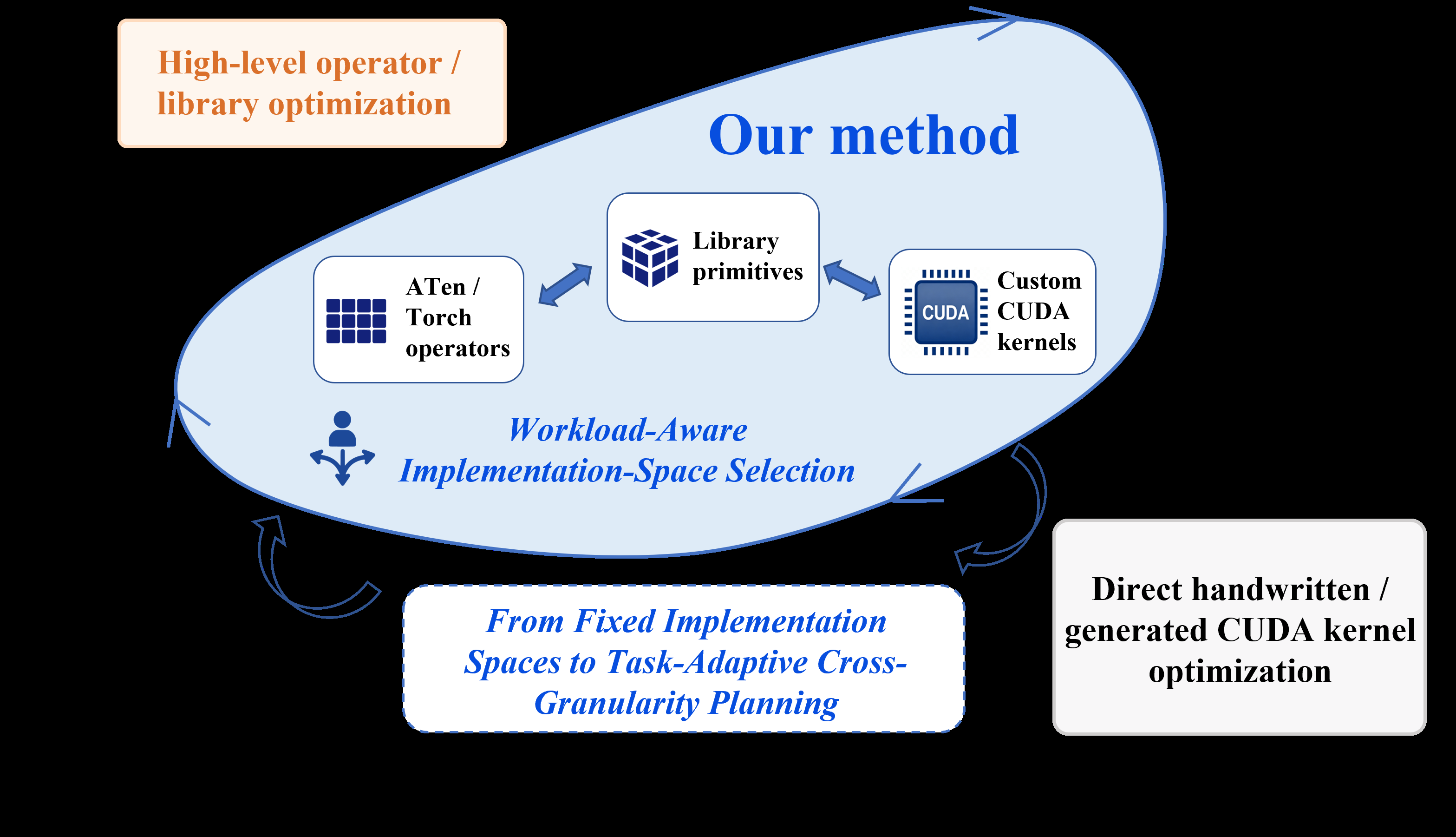
Figure 1 is the paper’s conceptual pitch, before any of the mechanism is introduced: existing methods sit either in the “high-level operator / library optimization” corner (safe, portable, capped upside) or the “direct handwritten / generated CUDA kernel” corner (highest ceiling, highest failure rate). HIERA’s claim is that the right move for a given workload is not always in the same corner — it should be chosen per-task, and even per-refinement-step, based on workload characteristics and profiling feedback.

4.1 Overall Architecture — Four Agents, One Feedback Loop

Figure 2: The HIERA Pipeline

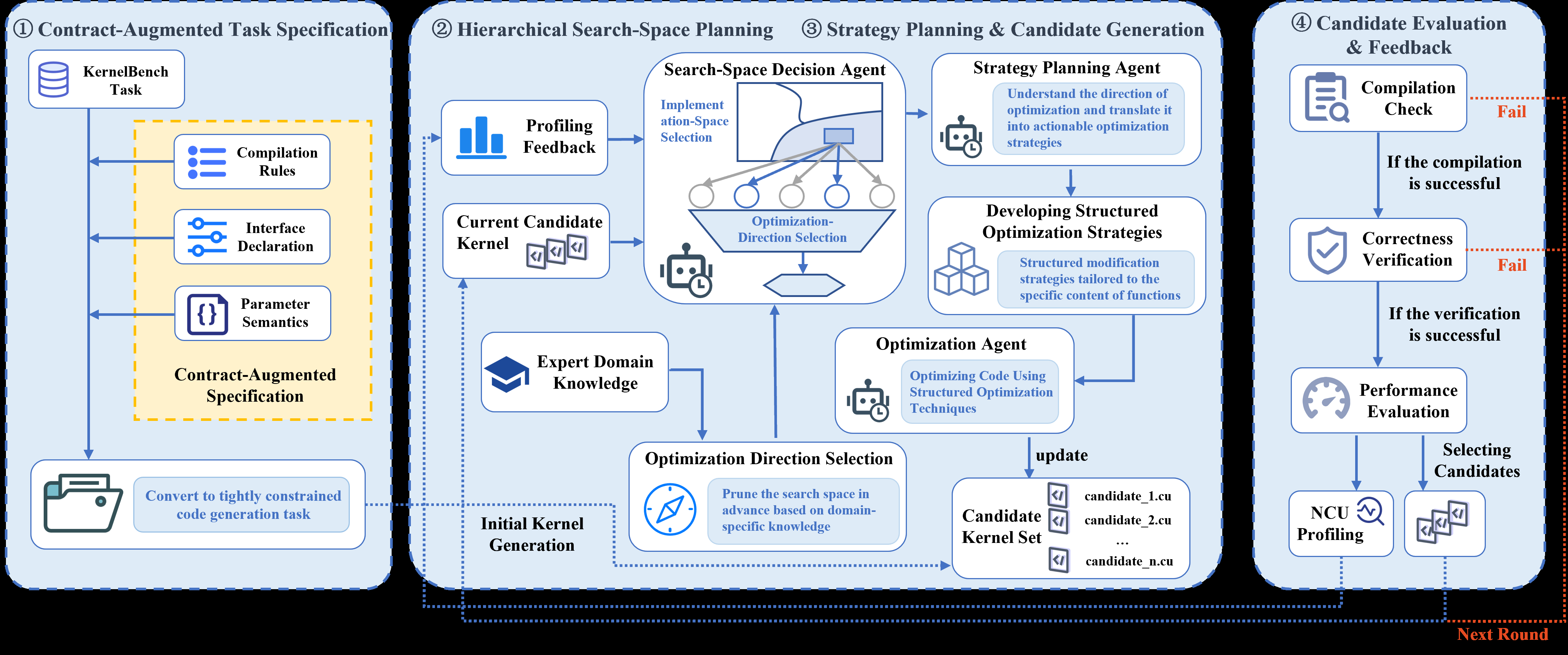
HIERA is organized as four cooperating components (the paper calls the two central ones “agents” — in practice, all four are LLM calls with different prompts/roles, orchestrated by a control loop):

1. Contract-Augmented Task Specification (a preprocessing step, not really an “agent” — deterministic).
2. Search-Space Decision Agent (SSDA) — decides where to search: which implementation space, and within it, which optimization direction.
3. Strategy Planning Agent (SPA) — translates the chosen direction into a concrete, actionable optimization strategy (specific code transformations).
4. Optimization Agent (OA) — actually writes the candidate kernel code implementing that strategy.

After generation, candidates go through compilation checking → correctness verification → performance evaluation → NCU profiling, and the results feed back into the next round’s SSDA call. Let’s unpack each piece, since this is exactly the kind of design that clause 15 of my writing guidelines asks me to break apart rather than gloss over.

4.2 Contract-Augmented Task Specification — Why Bother?

Here’s a subtle but important engineering point the paper makes: if you literally hand a raw KernelBench task to an LLM and say “write a fast version,” the model has to also reconstruct a pile of boilerplate that has nothing to do with optimization — host-side Python wrappers, PyTorch C++ extension bindings, input-generation/test-harness code, and the reference implementation’s exact calling convention. Every token spent regenerating that boilerplate is a token not spent reasoning about the actual optimization, and every place the model deviates from the expected interface (wrong argument order, wrong return type, wrong dtype) is a new way for the candidate to fail compilation or correctness checking for reasons that have nothing to do with whether the optimization idea was good.

HIERA’s fix: for every task, freeze a set of contract files that the model never has to (and is not allowed to) regenerate:

• torch_demo.py — the PyTorch-extension wrapper.
• cpp_source.cpp — the C++ binding source connecting Python to the CUDA kernel.
• groundtruth.py — the correctness reference.
• params_semantics.json — only for Level 2/3 tasks — a structured description of argument roles, shapes, constraints, and dependencies between parameters (Level 1 tasks skip this file because a single operator’s parameter semantics are inferable directly from its interface).

Given these fixed artifacts, the LLM’s job narrows to producing exactly one file: cuda_source.cu, containing the candidate implementation, via a structured response format. This is then automatically stitched together with the frozen contract files and compiled through the standard KernelBench harness.

Design-choice discussion — why this works, the obvious alternative, and where it can fail:

• Why it works: it removes an entire class of “correct optimization idea, wrong plumbing” failures, and it makes the LLM’s context budget go further, since it isn’t re-deriving unchanging boilerplate every round.
• The obvious alternative: let the model generate a complete, self-contained runnable program each time (what KernelBench-Caesar effectively does). This is simpler to implement but, per the ablation in Section 6.4, costs dearly on validity for the harder task levels.
• Where it can fail: the contract is only as good as params_semantics.json’s coverage. If the auto-derived parameter semantics for a Level 2/3 task are subtly wrong (e.g., mis-describing a broadcasting rule), the contract itself becomes a source of correctness bugs that the model has no way to detect or override — a failure mode the paper does not discuss (more on this in Section 9).

4.3 Cross-Granularity Search-Space Planning — the Central Mechanism

This is HIERA’s headline idea, formalized as follows. At each refinement step $t$, the Search-Space Decision Agent (SSDA) selects one of three nested implementation spaces, ordered by increasing permissiveness:

1. Pure CUDA — only custom, handwritten CUDA kernels are allowed.
2. CUDA Libraries — additionally permits calling optimized vendor libraries (cuBLAS, etc.).
3. CUDA Libraries + PyTorch — additionally permits falling back to high-level PyTorch operators.

Note the nesting: space 3 ⊇ space 2 ⊇ space 1 in terms of what’s allowed, but this is inversely related to how much low-level control the agent has — space 1 gives maximum control but maximum implementation burden; space 3 gives minimum burden but caps how much can be squeezed out through custom fusion/tiling.

Denote the selected space at step $t$ as $g_t$. This choice matters before any code is written, because it changes what the Optimization Agent is even allowed to propose — for a composite Level-3 workload, choosing $g_t =$ “CUDA Libraries + PyTorch” upfront means the agent doesn’t have to spend its limited budget re-deriving the operator dependency graph and intermediate data flow from scratch in raw CUDA; it can compose known-good building blocks and reserve custom-CUDA effort for the one or two genuinely bottlenecked sub-operations.

4.4 Domain-Guided Optimization-Direction Pruning

Within whichever space $g_t$ was selected, HIERA further narrows the search by choosing an optimization direction from a fixed taxonomy of five recurring GPU-performance bottleneck categories, distilled from prior GPU-optimization literature and expert practice:

• C — Control-flow and boundary specialization: eliminating warp divergence from conditional branches, specializing boundary-handling code paths (e.g., separate kernels for interior vs. edge tiles in a stencil) so the common case avoids branch overhead.
• P — Thread- and warp-level parallelism: ensuring enough independent work is exposed to saturate the GPU’s SMs — e.g., increasing grid/block dimensions, restructuring loops to expose more parallel work per thread.
• M — Memory transaction efficiency: coalescing global memory accesses, avoiding bank conflicts in shared memory, aligning access patterns to hardware transaction granularity.
• R — Data reuse and data-movement pipelining: tiling to maximize on-chip (shared memory/register) reuse of loaded data, and overlapping compute with memory transfers (double buffering, cp.async-style pipelining).
• T — Tensor Core and instruction-pipeline utilization: restructuring computation to hit hardware matrix-multiply-accumulate (mma) units, or improving instruction-level pipelining/scheduling to avoid stalls.

Let $D = \{C, P, M, R, T\}$. At step $t$, the SSDA scores every direction using the task specification $\tau$, the selected space $g_t$, the current candidate $x_t$, profiling feedback $F_t$ (from NCU), curated expert knowledge $E$, and a fixed scoring rubric $R$:

$$s_t = \text{SSDA}(\tau, g_t, x_t, F_t, E; R) = \big(s_t^d\big)_{d \in D} \tag{3}$$

i.e., the output is a vector of five relevance scores, one per direction. The primary direction chosen for this step is simply the argmax:

$$d_t^{*} = \arg\max_{d \in D} s_t^{d} \tag{4}$$

Design-choice discussion: why a fixed, five-category taxonomy rather than letting the model freely describe whatever bottleneck it perceives in natural language? The fixed taxonomy makes the direction-selection step structured and comparable across steps — the SSDA’s five scores are directly analogous to a lightweight classification head, which (a) makes the decision auditable/loggable in a consistent schema, and (b) lets the downstream Strategy Planning Agent draw on a matching library of expert-curated strategies indexed by exactly these five categories (see next section), rather than having to interpret arbitrary free-text bottleneck descriptions. The obvious alternative — free-form bottleneck diagnosis — is strictly more expressive (a workload might genuinely be bottlenecked by something the five categories don’t cleanly capture, e.g. instruction-cache pressure or atomic-contention on cross-block reductions) but sacrifices this structure. The paper is explicit that the taxonomy is “operational rather than exhaustive,” i.e., the authors acknowledge this is a practical five-bucket approximation of a much richer bottleneck space, deliberately trading completeness for reliability of downstream strategy retrieval.

4.5 Strategy Planning Agent — From Direction to Actionable Strategy

Given the primary direction $d_t^{*}$, the Strategy Planning Agent (SPA) produces a concrete, structured strategy:

$$\pi_t = \text{SPA}(\tau, g_t, x_t, F_t, d_t^{*}, E), \quad \pi_t \in \Pi_{g_t, d_t^{*}} \tag{5}$$

Here $\Pi_{g_t, d_t^*}$ denotes the space of strategies that are valid given the current implementation space and direction — e.g., a “restructure for Tensor Core mma utilization” strategy ($d^* = T$) is only meaningful if $g_t$ = Pure CUDA or CUDA Libraries (Tensor Core intrinsics aren’t something you invoke from a plain PyTorch call). This constraint-typing of the strategy space is what prevents the SPA from proposing something the OA structurally cannot execute given the chosen space.

4.6 Optimization Agent — Generating the Next Candidate Batch

Finally, the Optimization Agent (OA) takes the strategy $\pi_t$ and applies it, generating the next batch of candidate kernels:

$$X_{t+1} = \text{OA}(\tau, g_t, x_t, F_t, \pi_t) \tag{6}$$

Note this produces a set $X_{t+1}$ of candidates (not a single one) — HIERA’s experiments use a “population” style loop where multiple candidates are generated per round (six per round in the main comparison protocol) and the survivors are carried forward as parents for the next round.

4.7 Feedback-Driven Evaluation Loop, Written Out as Pseudocode

Putting Sections 4.2–4.6 together, here is the full HIERA loop, spelled out step-by-step (my own reconstruction from the paper’s prose description, not verbatim from the paper, since the paper describes this loop across several sub-sections rather than as a single algorithm block):

Algorithm 1: HIERA Optimization Loop
Input:  task τ, reference f_τ, hardware H, total budget B,
        rounds R, candidates-per-round K  (paper: R=3, K=6, B=RK=18)
Output: best valid candidate x*_τ found within budget

 1: spec  ← ContractAugment(τ)                 # freeze wrapper/binding/reference files
 2: x_0   ← InitialCandidate(spec)              # seed candidate (e.g. naive translation)
 3: g_0   ← SSDA.select_space(spec, x_0, F=∅, E)   # first implementation-space choice
 4: best  ← x_0 if Valid(x_0; τ) else NONE
 5: for t = 0 .. R-1:
 6:     s_t     ← SSDA.score_directions(spec, g_t, x_t, F_t, E; R)   # Eq. 3
 7:     d*_t    ← argmax_d s_t[d]                                     # Eq. 4
 8:     π_t     ← SPA.plan(spec, g_t, x_t, F_t, d*_t, E)              # Eq. 5
 9:     X_{t+1} ← OA.generate(spec, g_t, x_t, F_t, π_t, K)            # Eq. 6, K candidates
10:     for each candidate x in X_{t+1}:
11:         if not Compiles(x, spec):           continue   # discard: compile failure
12:         if not Valid(x; τ):                 continue   # discard: wrong output
13:         measure t(x; τ, H) on H                          # latency
14:         F_x ← NCU_profile(x, H)                          # hardware counters
15:         compute s(x; τ, H) = t(f_τ;H) / t(x;τ,H)          # Eq. 1
16:         if best is NONE or s(x;τ,H) > s(best;τ,H):
17:             best ← x
18:     x_{t+1} ← best-of-round(X_{t+1})        # strongest surviving candidate as new parent
19:     F_{t+1} ← NCU_profile(x_{t+1}, H)       # feedback carried into next round's SSDA call
20:     g_{t+1} ← SSDA.select_space(spec, x_{t+1}, F_{t+1}, E)   # re-decide space each round
21: return best

A few things worth calling out explicitly, since they’re easy to miss on a first read of the paper:

• The implementation-space decision is re-made every round (line 20), not fixed once at the start. This means HIERA can, e.g., start a Level-3 task in the permissive “CUDA Libraries + PyTorch” space to quickly get something valid and measured, then progressively narrow toward “Pure CUDA” for the specific sub-operation profiling reveals as the bottleneck — a coarse-to-fine strategy the paper explicitly frames as its intended usage pattern.
• Invalid candidates are silently discarded, not penalized or “explained away.” There is no soft credit for a nearly-correct-but-not-quite candidate; per the Eq. (2) formulation, only valid candidates compete on speed at all.
• The budget accounting is entirely candidate-count-based ($B = R \times K$), not wall-clock-time-based — this matters for interpreting the “budget $B \in \{1, 6, 12, 18\}$” curves in Section 6, since those are extracted retrospectively from the same generation trajectories rather than independently re-run with different budgets.

5. Experimental Setup

• Benchmark: all three KernelBench levels (250 tasks total: 100 / 100 / 50 for Levels 1/2/3).
• Base LLMs: DeepSeek-V3.2, Qwen3.6-Plus, Gemini-3.6-Flash — three different underlying models, to test whether HIERA’s benefit is model-agnostic (a training-free method should, in principle, transfer across base models without retraining, unlike CUDA-L1/Kevin).
• Baselines: KernelBench-Caesar (the unconstrained iterative baseline), CUDAForge (the fixed pure-CUDA agentic baseline), and CUDA-L1 (the RL-trained baseline, reported once since it doesn’t vary by base LLM).
• Budget: $R = 3$ refinement rounds, $K = 6$ candidates/round, for a maximum $B = 18$ candidates per task, with cumulative results also reported at smaller sub-budgets $B \in \{1, 6, 12\}$ by truncating the same trajectories.
• Hardware: a single NVIDIA A100-PCIe-40GB per task (Table 1 in the paper gives full software versions: CUDA 12.8, PyTorch 2.7.1, cuDNN 9.5.1).
• Evaluation protocol: each valid candidate is benchmarked in FP32 with 3 warm-up runs followed by 100 measurement runs; the fastest valid candidate within the full budget is reported.

Two additional controlled studies isolate specific design components:

• Implementation-space comparison (RQ2, cross-granularity): on 90 sampled tasks (30 per level), HIERA is compared against three fixed-space variants — always Pure CUDA, always CUDA Libraries, always CUDA Libraries + PyTorch — with every other setting (base LLM = Qwen3.6-Plus, contract specification, direction-planning procedure, budget) held constant. This isolates the marginal value of adaptive space selection, holding everything else fixed.
• Ablations: “HIERA w/o Contract” (drops the frozen-artifact specification, forcing the model to regenerate boilerplate) and “HIERA w/o Planning” (drops the hierarchical SSDA/SPA planning entirely, replacing it with one fixed, unconstrained optimization prompt).

6. Results

6.1 RQ1 — Main Comparison: Sample Efficiency and Overall Quality

Figure 3: Limited-Budget Performance Curves

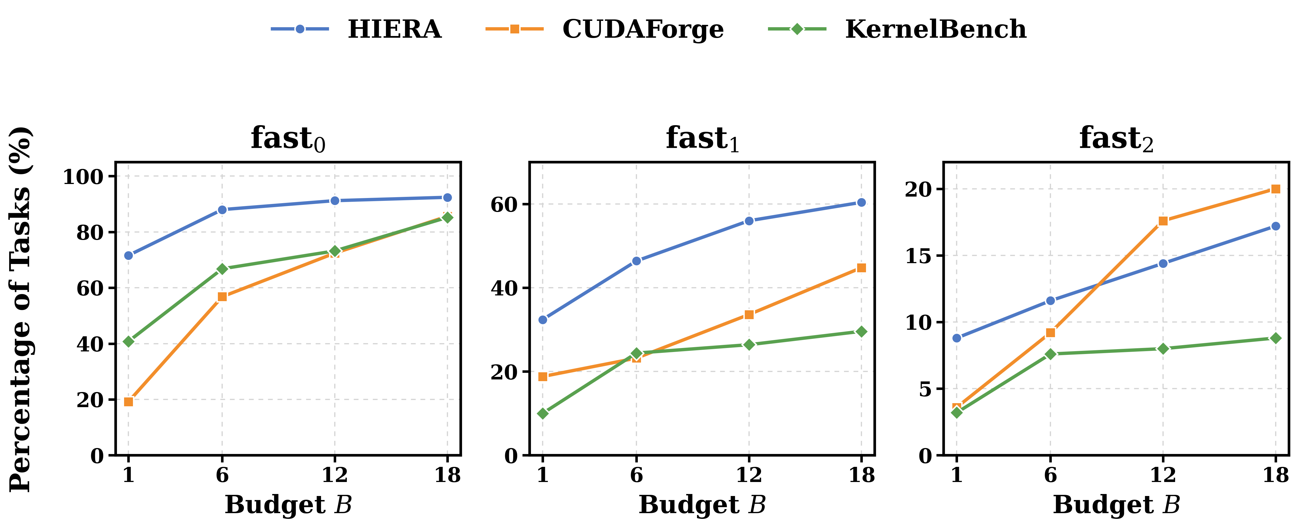
The headline number: at $B=1$ (i.e., after generating just a single candidate, before any iterative refinement at all), HIERA already achieves $71.6\%$ $\text{fast}_0$ and $32.4\%$ $\text{fast}_1$ — beating KernelBench-Caesar by $+30.8$ and $+22.4$ percentage points respectively, and CUDAForge by $+52.4$ and $+13.6$ points. This is a striking result: it says that HIERA’s very first guess, informed by its space-and-direction planning step, is already dramatically more likely to be both valid and fast than a full round of iterative refinement from the baselines. This advantage persists but narrows somewhat at $B=18$: HIERA reaches $92.4\%/60.4\%$ vs. KernelBench-Caesar’s $85.2\%/29.6\%$ and CUDAForge’s $85.6\%/44.8\%$.

Interestingly, on the stricter $\text{fast}_2$ metric ($>2\times$ speedup), HIERA’s lead is present but smaller and, at large budgets, CUDAForge actually catches up and slightly surpasses HIERA (see Table 2 below and the boxplot in Figure 4) — a nuance the paper reports honestly rather than glossing over, and one I’ll return to in the critical analysis (Section 9), because it complicates the “HIERA is strictly better” narrative.

6.2 Cross-Model Comparison (Table 2, reproduced and discussed)

Base LLM	Method	L1 fast0/fast1/fast2	L2 fast0/fast1/fast2	L3 fast0/fast1/fast2
DeepSeek-V3.2	HIERA	91/56/22	90/35/9	64/42/10
DeepSeek-V3.2	KernelBench-Caesar	77/17/3	80/34/5	46/12/2
DeepSeek-V3.2	CUDAForge	90/22/6	78/27/15	60/32/10
Qwen3.6-Plus	HIERA	97/68/18	99/62/20	70/42/10
Qwen3.6-Plus	KernelBench-Caesar	91/21/6	90/40/13	64/26/6
Qwen3.6-Plus	CUDAForge	90/47/18	88/45/28	72/40/8
Gemini-3.6-Flash	HIERA	95/63/20	96/50/14	68/40/12
Gemini-3.6-Flash	KernelBench-Caesar	80/19/4	85/32/11	52/14/2
Gemini-3.6-Flash	CUDAForge	92/45/16	91/40/20	70/34/8
(any)	CUDA-L1 (RL-trained)†	74/19/10	81/36/13	72/50/6

†CUDA-L1 does not vary with the base-LLM column and is reported once.

Reading this table carefully (rather than just quoting the paper’s summary “best or tied-best in 22 of 27 comparisons”) reveals genuine texture: HIERA’s advantage is largest and most consistent on $\text{fast}_1$ across every base model and level — it is the strongest system at “did this actually get faster than the reference” in all nine level×model combinations shown. But on $\text{fast}_2$ (the $>2\times$ bar), CUDAForge wins outright on DeepSeek-V3.2/L2 (15 vs 9), Qwen3.6-Plus/L2 (28 vs 20), and Gemini-3.6-Flash/L2 (20 vs 14) — in every case on Level 2 specifically. And CUDA-L1, despite requiring no per-task planning at all, wins outright on Level-3 $\text{fast}_2$ (6% vs HIERA’s 10% — wait, HIERA actually wins there too when compared to CUDA-L1’s 6%, but CUDA-L1 wins L3 fast1 at 50% vs HIERA’s best of 42%). So a fair reading is: HIERA is the best all-around, most-reliable system, but it does not universally dominate every metric on every level — the RL-trained CUDA-L1 retains an edge on the hardest ($\text{fast}_2$, Level 3) tail, likely because its training process specifically optimizes for exactly that objective (deep, aggressive CUDA rewrites) at the cost of the generality HIERA provides.

6.3 RQ2 — Isolating the Value of Adaptive Space Selection

Figure 4: Speedup Distribution by Fixed vs. Adaptive Implementation Space

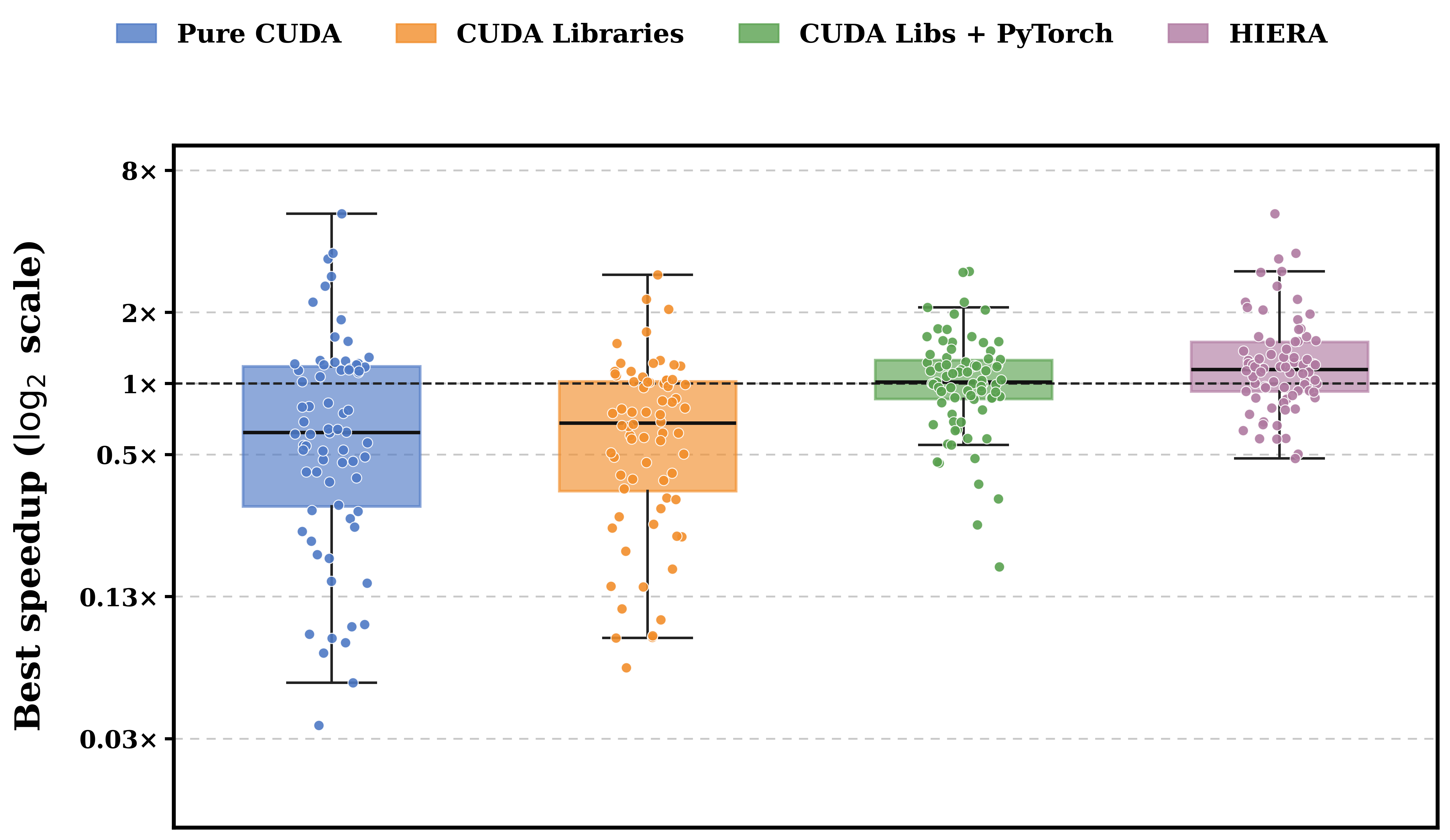
This is, in my view, the most information-dense figure in the paper, and it directly supports the core thesis. Reading the box-and-swarm plot:

• Pure CUDA (always-custom-CUDA) has the highest ceiling — its maximum observed speedup is $9.32\times$, the best single number in the whole comparison — but its mean is only $1.00\times$ and its median is $0.62\times$ (i.e., for the typical task, “always write raw CUDA” is actually a net slowdown relative to the PyTorch reference!), with the largest variance (1.79). This is the empirical evidence behind the paper’s motivating claim: unconstrained low-level search burns budget on implementations that end up worse than doing nothing.
• CUDA Libraries (allowing library calls) roughly halves the variance (to 0.27) versus Pure CUDA but keeps a similarly modest mean/median.
• CUDA Libraries + PyTorch (most permissive, framework-heavy) achieves the lowest variance (0.26) and improves mean/median to $1.10\times$/$1.01\times$, but its observed ceiling caps out at $2.98\times$ — safety comes at the cost of upside.
• HIERA (adaptive) achieves the best of both worlds on the aggregate statistics: highest mean ($1.42\times$) and highest median ($1.15\times$) among all four, while cutting variance by $23.4\%$ relative to Pure CUDA — i.e., it captures much of Pure CUDA’s upside potential (its swarm plot shows several points above $2\times$, up to a maximum near $5\times$) while avoiding the “worse than doing nothing” tail that plagues the fixed-Pure-CUDA strategy.

Design-choice discussion: this figure is the strongest evidence in the paper, and it’s worth being precise about why it’s convincing: it’s a controlled experiment (same 90 tasks, same base LLM, same everything except the space-selection policy), so the difference is attributable specifically to the adaptivity, not to some confound like a stronger base model or a bigger budget. The obvious alternative to this ablation design would be a full head-to-head against a completely different agent framework, but that would conflate “does adaptive space selection help” with “is this framework’s prompt engineering/orchestration better overall” — the controlled 90-task comparison isolates the one variable the paper wants to claim credit for.

6.4 Ablation Studies

Figure 5: Ablating the Contract-Augmented Specification

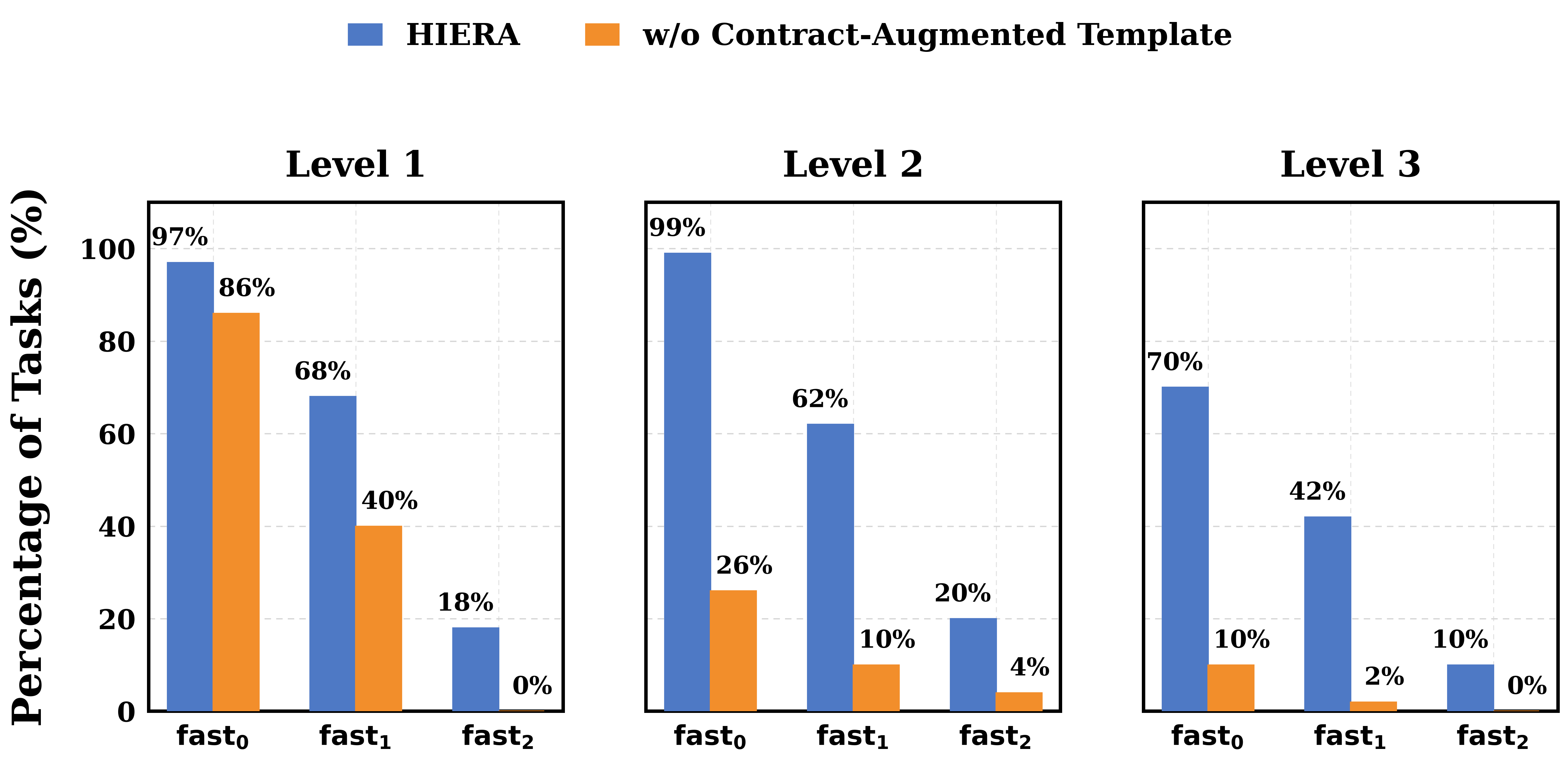
Removing the frozen contract files (“w/o Contract-Augmented Template”) degrades performance at every level, but the size of the degradation scales sharply with task complexity: Level 1’s $\text{fast}_0$ drops from 97% → 86% (an 11-point hit, tolerable), but Level 2 drops 99% → 26% (a 73-point collapse) and Level 3 drops 70% → 10% (a 60-point collapse). The intuition: Level 1 tasks are single operators, so even without a frozen contract, there isn’t much boilerplate to get wrong; Level 2/3 tasks require reconstructing complex operator dependency graphs and multi-file bindings from scratch, and that reconstruction is exactly where models go wrong when they aren’t given a fixed scaffold.

Figure 6: Ablating Hierarchical Search-Space Planning

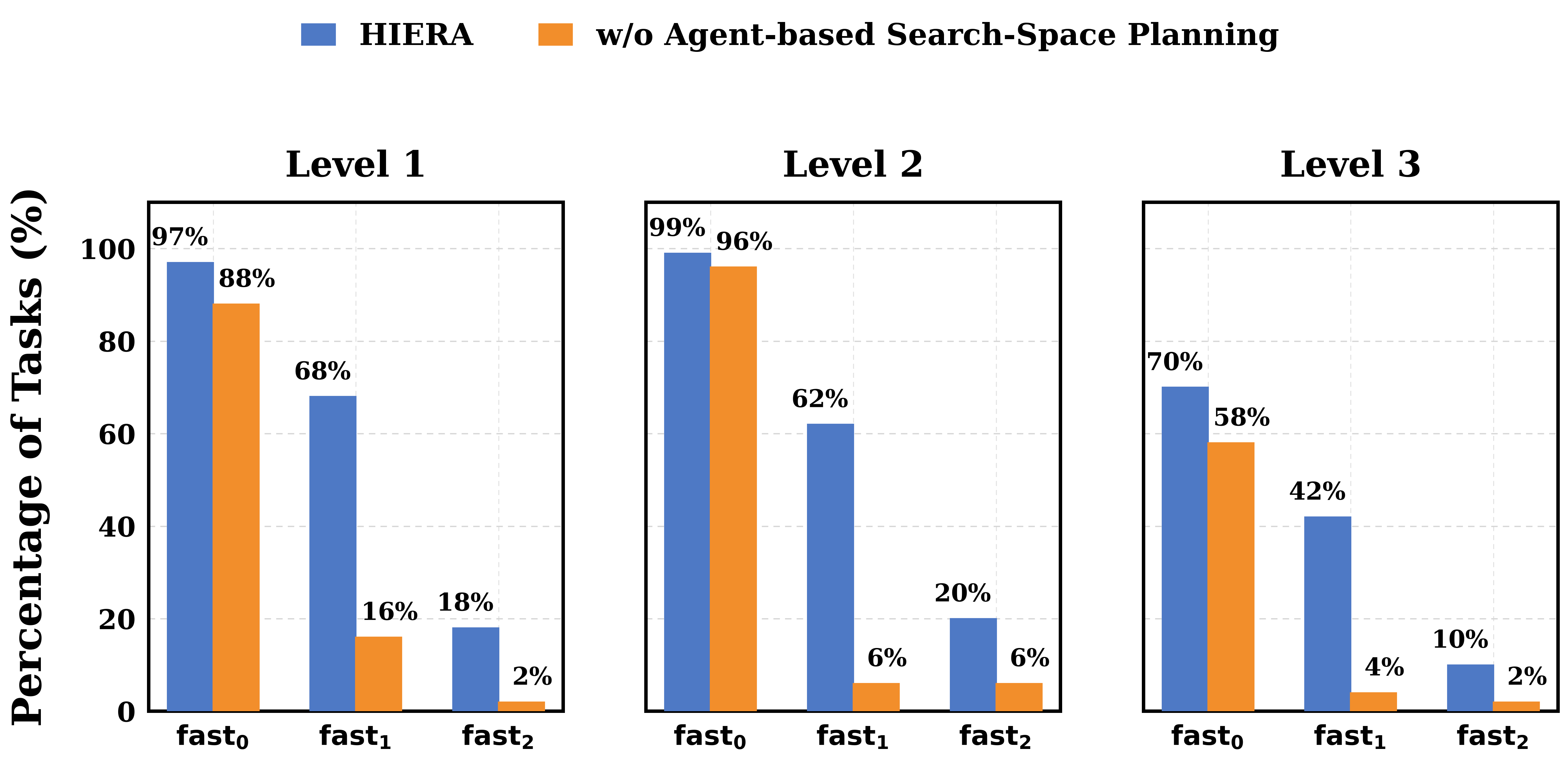
This ablation tells the opposite story, and the contrast between Figures 5 and 6 is itself instructive. Removing hierarchical planning (replacing it with one fixed, unconstrained optimization prompt) barely touches $\text{fast}_0$ (Level 2: 99% → 96%, a mere 3-point drop) — the model can still usually produce something valid without guidance. But $\text{fast}_1$ and $\text{fast}_2$ collapse: Level 2 $\text{fast}_1$ falls from 62% → 6%, and Level 1 $\text{fast}_1$ drops by 52 points, Level 3 by 38 points. In other words: planning doesn’t primarily help you produce working code — it helps you produce working code that is also actually faster. The paper’s own summary captures this nicely: “contract augmentation primarily preserves feasibility, whereas hierarchical planning improves acceleration” — these two components address genuinely different failure modes, which is a satisfying, falsifiable claim (and it’s nice that the paper’s ablation design was set up in a way that could have shown these two components doing the same thing, but empirically didn’t).

6.5 RQ3 — Case Study: A Stencil Computation from Scientific Computing

Figure 7: Beyond ML Workloads — a 2D Box Stencil

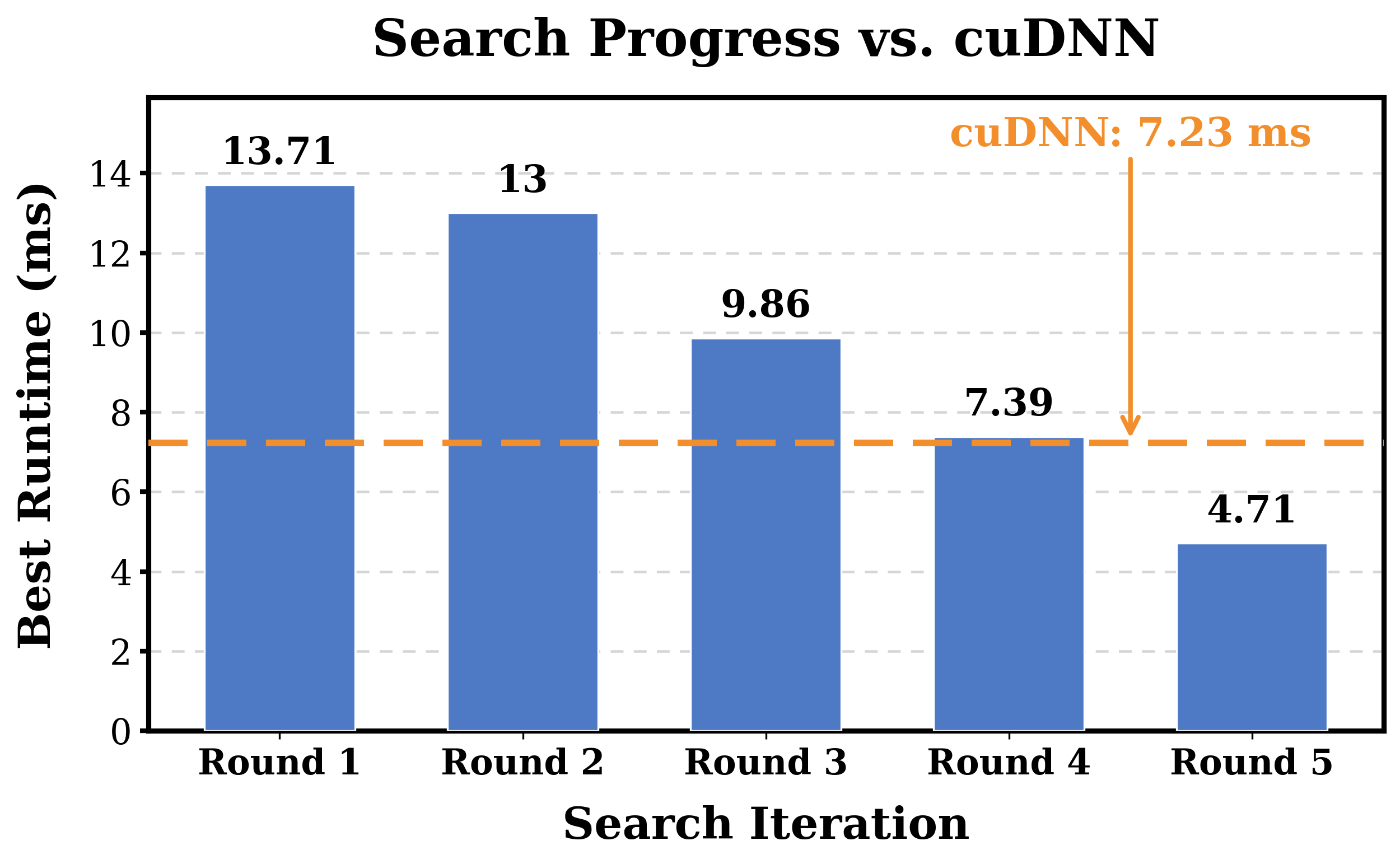
This is a nice generality check: the paper steps outside KernelBench entirely to ask whether HIERA’s approach transfers to non-ML GPU workloads. The task: a 2D box stencil with radius $R=3$ (a $7\times 7 = 49$-point neighborhood), input size $10240 \times 10240$, repeated $10{,}240$ times, with per-step latency reported (amortized). The chosen dense-computation baseline is cuDNN’s cudnnConvolutionForward, configured as a single-channel $7\times7$ zero-padded cross-correlation in FP64 — a legitimate way to compute a stencil via convolution, and a genuinely strong, vendor-tuned reference (7.23 ms/step).

Search proceeds over 5 rounds with population size 10 (total budget 50 candidate evaluations — notably larger than the $B=18$ used in the main KernelBench comparison, since this is a single deep-dive case study rather than a broad benchmark run). Runtime falls monotonically: $13.71 \to 13.00 \to 9.86 \to 7.39 \to 4.71$ ms. The candidate doesn’t beat cuDNN until round 5, where it lands at 4.71 ms — a $34.8\%$ improvement over cuDNN, i.e., a $1.53\times$ speedup, and a $65.6\%$ reduction from the very first candidate.

Design-choice discussion — is this a fair comparison? The paper is explicit and appropriately modest here: it frames this as “evidence of feasibility rather than comprehensive validation,” and rightly so — this is one operator, one configuration, one GPU. A stencil with $R=3$ has a specific, favorable structure for shared-memory tiling (regular, small, symmetric neighborhood) that plays directly into where custom CUDA tends to beat generic dense-convolution formulations; it would be a different (and much harder) test to try, say, a stencil with a highly irregular or data-dependent access pattern, or a genuinely large-radius stencil where register/shared-memory pressure becomes a binding constraint.

7. Limitations (as Stated by the Authors)

The paper’s own “Scope and Limitations” section is commendably direct, and I’ll enumerate it faithfully before adding what I think it leaves out (Section 9):

1. Single GPU architecture: all experiments run on NVIDIA A100 GPUs; performance characteristics (occupancy targets, memory-bandwidth-to-compute ratios, Tensor Core generation) differ meaningfully on H100/B200-class hardware, and the paper does not claim the learned direction taxonomy or space-selection heuristics transfer without re-validation.
2. Single precision format for the main benchmark: KernelBench evaluation uses FP32 throughout; the stencil case study uses FP64. Lower-precision formats (FP16/BF16/FP8), which dominate real LLM training/inference workloads, are explicitly flagged as unexplored.
3. No multi-GPU evaluation: every task is assigned to a single GPU; multi-GPU kernels (which introduce inter-GPU communication as a new, dominant cost axis) are out of scope.
4. Stochasticity of candidate generation: the paper notes latency measurements are repeated (3 warmup + 100 measurement runs) to control for hardware/measurement noise, but candidate generation itself remains stochastic — re-running the same pipeline could plausibly produce a different trajectory, and the paper does not report variance across repeated end-to-end runs (as opposed to variance across the 90 sampled tasks within one run).
5. The stencil case study is a single operator/configuration, explicitly described as “feasibility” evidence rather than a validated general capability for scientific-computing workloads.

8. Reproducibility Notes

• Benchmark/tasks: KernelBench is publicly available (github.com/ScalingIntelligence/KernelBench); the 250 tasks and their reference implementations are open.
• Base models: DeepSeek-V3.2 and Qwen3.6-Plus are accessible via API/open weights depending on release terms; Gemini-3.6-Flash is API-only — full bit-exact reproduction requires access to the exact model snapshots used (which can drift/deprecate over time on hosted APIs — a common reproducibility hazard for any paper benchmarking against commercial LLM endpoints).
• Hardware: the paper specifies A100-PCIe-40GB, driver 565.57.01, CUDA 12.8, PyTorch 2.7.1+cu126, cuDNN 9.5.1 (Table 1) — this level of detail is good practice and should make like-for-like re-runs on comparable hardware plausible.
• Not released (as of this review): the paper does not mention a public code/artifact release for HIERA’s own orchestration code (the SSDA/SPA/OA prompts, the contract-generation tooling, or the params_semantics.json derivation process), which is the actual novel artifact of this work. Without that, independent reproduction requires re-implementing the four-agent loop and the five-direction expert-knowledge base from the paper’s prose description alone — feasible (I did exactly that to write Algorithm 1 above) but nontrivial, and almost certainly not bit-for-bit identical to the authors’ internal prompts.
• Sampling temperature: fixed at 0.3 across methods for fairness — worth preserving if attempting a re-run, since kernel-generation quality is sensitive to sampling temperature in ways that are easy to accidentally vary between conditions.

9. Critical Analysis

(a) Weaknesses and flaws specific to this paper.

• The headline “22 of 27 comparisons” framing partially obscures a real, level-specific weakness. As I traced out in Section 6.2, HIERA loses to CUDAForge on $\text{fast}_2$ specifically on Level 2, across all three base LLMs — not a one-off fluke. Level 2 (fused multi-operator patterns) is arguably the level where “compose CUDA libraries with light custom fusion” (HIERA’s adaptive approach) trades off against “go all-in on custom CUDA fusion” (CUDAForge’s approach) most directly, and the data suggests that for the specific goal of “extreme” ($>2\times$) speedups, committing hard to custom CUDA can still win. The paper’s summary statistic (“22 of 27”) is technically accurate but a reader skimming only the abstract/conclusion would not learn that this loss is systematic and level-specific rather than noise.
• The five-direction taxonomy’s coverage is asserted, not measured. The paper states the $\{C, P, M, R, T\}$ taxonomy is “operational rather than exhaustive,” which is an honest hedge, but there’s no experiment quantifying how often the SSDA’s actual bottleneck diagnosis (from NCU profiling) falls outside all five categories, or what happens when it does — does the SSDA just pick the least-bad-fitting category, silently degrading strategy quality? This would have been a cheap, illuminating experiment: log the raw NCU stall-reason breakdown for a sample of tasks and check how often it maps cleanly onto one of the five buckets.
• “90 sampled tasks” for the headline cross-granularity comparison (Figure 4) is 36% of the full 250-task suite, and the sampling procedure (“30 tasks from each of Levels 1–3”) is described as random but the actual random seed / task IDs are not listed in the paper, which matters for exact reproduction of Figure 4 specifically (as opposed to the main Table 2 results, which use the full 250-task suite).
• No confidence intervals or statistical significance testing anywhere in the results. Every number in Table 2 and the RQ1/RQ2 figures is a point estimate from a single run per (method, base-LLM, level) combination. Given that candidate generation is explicitly acknowledged (in the Limitations section) to be stochastic, and that several of the reported gaps between methods are in the single-digit percentage-point range (e.g., DeepSeek-V3.2/L3: HIERA 64% vs CUDAForge 60% $\text{fast}_0$ — a 4-point gap), it’s genuinely unclear which differences would survive a repeated-run variance analysis.

(b) Limitations the authors understate or omit.

• Cost/latency of the four-agent pipeline itself is never reported. HIERA makes (at minimum) one SSDA call, one SPA call, and one OA call per refinement round per task, plus NCU profiling overhead — this is meaningfully more LLM-inference cost per candidate than a single “generate and check” baseline like KernelBench-Caesar. The paper reports zero numbers on wall-clock time-to-result, total token cost, or dollar cost of running HIERA vs. the baselines at matched budget $B$. For a paper whose entire premise is about efficient use of a limited budget, budget measured purely in “candidate count” while ignoring the very different per-candidate cost of a four-LLM-call pipeline vs. a single-call baseline is a real gap — it’s plausible that at matched compute/dollar budget (rather than matched candidate-count budget), some of HIERA’s advantage would shrink, since each of its candidates costs more to produce.
• The interaction between the contract-augmentation ablation and the planning ablation is not tested jointly. We know contract-alone matters a lot (Figure 5) and planning-alone matters a lot (Figure 6), but there’s no reported “w/o both” condition, so we can’t tell whether their effects are additive, sub-additive (some overlap in what failures they each prevent), or even super-additive. This is a one-line addition to an already-run ablation grid.
• The paper doesn’t discuss what happens when the SSDA’s space/direction choice is simply wrong — e.g., it commits to “Pure CUDA” + direction “T” (Tensor Core) for a workload where Tensor Cores genuinely aren’t applicable (e.g., odd, non-tile-friendly shapes). Does the system recover within the remaining rounds via the profiling feedback loop, or can a bad early planning decision permanently waste budget? Given the small round count ($R=3$), a single bad early decision could plausibly dominate the whole trajectory, and the paper provides no failure-case analysis to check.

(c) Concrete, specific improvement suggestions.

1. Report cost-normalized comparisons. Add a budget axis measured in total LLM tokens (or wall-clock seconds, or API dollars) alongside the existing candidate-count axis, and re-plot Figure 3 with that x-axis. This directly answers “is HIERA’s advantage still there at matched cost, not just matched candidate count” — the single most important missing piece of evidence for anyone trying to decide whether to adopt this in production.
2. Add a joint “w/o Contract AND w/o Planning” ablation cell to Figures 5/6’s comparison grid — trivial to run given the ablation infrastructure clearly already exists, and it directly answers the additivity question raised above.
3. Instrument and report SSDA “direction-taxonomy miss rate”: for a sample of tasks, compare the SSDA’s chosen direction against the raw NCU bottleneck classification, and report how often the top-scoring direction actually matches the empirically dominant stall reason. This would validate (or falsify) the taxonomy’s coverage claim with data instead of a qualitative hedge.
4. Extend the stencil case study to at least 3–5 operators/configurations spanning a spread of “how favorable is this to hand-written CUDA” (e.g., vary the stencil radius, try an irregular/data-dependent access pattern, try one workload where a library baseline is expected to win) — a single R=3 stencil case study, chosen without stating the selection criteria, invites the (fair) question of whether it was chosen because it was known in advance to be a good showcase.
5. Report repeated-run variance for at least the main Table 2 numbers on one representative (base-LLM, level) cell — even 3 repeated runs would let readers gauge whether the smaller reported gaps (single-digit percentage points) are meaningful or within noise.

10. Conclusion

HIERA’s central contribution is a reframing, not a new low-level optimization trick: it argues, and backs with a genuinely controlled ablation (Figure 4), that which abstraction level to search in is itself the highest-leverage decision available to a budget-constrained LLM kernel-optimization agent — more leverage, in fact, than how you search within a fixed level. Combined with a pragmatic, low-friction fix for boilerplate-induced correctness failures (the contract-augmented specification), this training-free system beats prior training-free baselines broadly and even edges out an RL-trained baseline (CUDA-L1) on most metrics without any weight updates. The honest caveats — a level-specific loss on the strictest speedup bar, unreported cost overhead of the four-agent pipeline, and a single-operator generality case study — mean this is best read as convincing evidence for a design principle (treat granularity as a decision, not a constant) rather than a finished, drop-in production tool. If you’re building or evaluating agentic kernel-optimization systems, the actionable takeaway is concrete: don’t hardcode your agent to one implementation altitude, and if you do give it the freedom to choose, measure the distribution of outcomes (mean/median/variance), not just the best-case ceiling — Figure 4’s boxplot is the single most useful figure in the paper precisely because it makes that distributional argument impossible to miss.