Review date: 2026-09-02 | Author: Zhongzhu Zhou Paper reviewed: Verification-Aware Training for Speculative Decoding Paper authors: Geonmo Gu, Byeongho Heo, HeeJae Jun, Yoohoon Kang, Sangmin Lee, Sangdoo Yun, Dongyoon Han (NAVER AI Lab, NAVER AI Search Platform, Korea University) arXiv: 2608.30135 Venue/Status: Preprint, submitted 31 Aug 2026
Why This Paper Matters
Every time you serve an LLM at any real scale, you eventually run into the same wall: autoregressive decoding forces one forward pass per output token, and forward passes are expensive. Speculative decoding (SD) has become the default fix — a small “drafter” model proposes a handful of candidate tokens cheaply, and the big “target” model verifies all of them in a single parallel forward pass, accepting a prefix and rejecting the rest. If the drafter is good, you get several tokens per big-model forward pass instead of one, and — this is the part people sometimes forget — the output distribution is provably identical to running the target model alone, token by token. It’s not an approximation; it’s free lossless speed, contingent entirely on how many draft tokens survive verification.
That “how many survive” number is called the acceptance length, and it is the single number that determines your speedup. The obvious next question a systems person should ask is: if acceptance length is what we care about, why do we train drafters on something else? This paper’s entire contribution flows from noticing that the standard training recipe for state-of-the-art drafters — EAGLE-3, DFlash, and basically everyone else — trains with plain per-position cross-entropy imitation of the target model, using a fixed, hand-picked decay schedule that discounts later positions a little, uniformly, for every training example, regardless of what actually happens during verification for that example. The training objective has no idea that verification is sequential (a rejection at position 3 makes positions 4, 5, 6… worthless regardless of their individual quality) and no idea where, for this particular sample, the rejection will actually occur.
Verification-Aware Training (VAT) closes that gap. It is a training-time-only, architecture-agnostic, inference-unchanged plug-in: you keep your existing drafter (autoregressive EAGLE-3 or diffusion-based DFlash), you keep the target model, you keep the inference procedure byte-for-byte — you only change what the loss function pays attention to during training. Applied on top of EAGLE-3 and DFlash across three target models (Qwen3-4B, Qwen3-8B, LLaMA-3.1-8B) and eight benchmarks spanning math, code, and chat, VAT improves average acceptance length by up to 11.4% and wall-clock speedup by up to 8.7%, for a training-time cost of roughly 1–6% extra compute per step and zero extra inference cost. That’s a genuinely rare kind of result in efficiency research: a free lunch on the inference side, paid for entirely (and cheaply) at training time.
flowchart LR
    subgraph SD["Standard speculative decoding (unchanged by VAT)"]
        D["Drafter proposes K tokens<br/>(cheap, autoregressive or parallel)"]
        V["Target verifies all K in parallel<br/>(one expensive forward pass)"]
        A["Accept prefix up to first rejection,<br/>resample the rest"]
        D --> V --> A
    end
    subgraph Train["What VAT changes: only the drafter's training loss"]
        T1["Old: fixed per-position weight<br/>w_k, same schedule for every sample"]
        T2["New: simulate verification during training,<br/>find first-rejection position k*, re-anchor weights there"]
        T3["New: add a verification head that<br/>predicts 'will this token survive verification?'"]
        T1 -.replaced by.-> T2
        T2 --> T3
    end
    A -.->|"acceptance length is what<br/>speedup actually depends on"| Train
Figure 1 (self-drawn): The core insight of this paper in one picture — speculative decoding’s speedup is entirely governed by acceptance length, but existing drafter training objectives ignore both the sequential, all-or-nothing nature of verification and where the rejection actually happens for each training example. VAT fixes exactly this training/inference mismatch without touching inference at all.
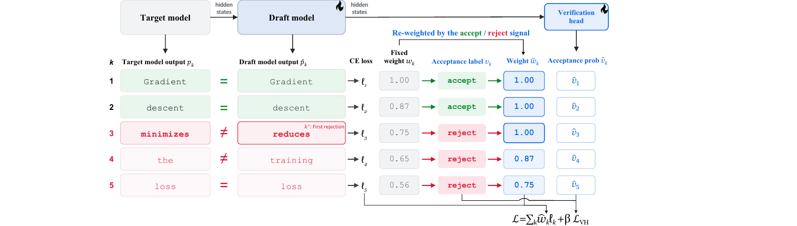
Figure 2 (paper Fig.1, original): The paper’s own diagram. At training step k, the target’s token (“minimizes”) and draft’s token (“reduces”) first disagree at position k*=3. Everything from k=3 onward gets an accept label of 0 (i.e., reject), which feeds into both a re-weighted per-position loss ŵ_k and a verification head that learns to predict acceptance probability v̂_k directly from the draft’s own hidden states.
Prerequisites
The mechanics of speculative decoding, precisely
Speculative decoding (Leviathan et al., 2023; Chen et al., 2023) accelerates autoregressive generation by splitting each decoding step into a drafting phase and a verification phase. Given a prefix, a lightweight draft model proposes candidate tokens autoregressively (or, for diffusion-style drafters like DFlash, in a single parallel forward pass). The target model then evaluates all candidates plus the actual prefix in one parallel forward pass — this parallelism is the entire reason SD is fast: verifying a fixed sequence of tokens costs about the same as verifying one token, on modern accelerators, because attention and matrix multiplies both parallelize over the sequence dimension. Verification then proceeds sequentially through the positions: at position , the drafted token is accepted with probability where are the target’s and drafter’s probabilities for token at that position, given the same prefix (this is standard rejection sampling, and it’s exactly what makes SD’s output distribution match running alone). The first time a token is rejected, every subsequent drafted token is discarded regardless of how “good” it individually was — that’s the crucial and easy-to-underappreciate detail — and a corrected token is resampled from the residual distribution at that position, after which a new drafting round starts from there.
The number of tokens accepted per verification cycle is the average acceptance length, denoted in this paper. Since every verification cycle has roughly fixed overhead (one target forward pass), a higher directly means fewer verification cycles per generated token and hence higher throughput. This is the single most important quantity in the whole SD literature, and it’s the quantity this paper’s method is built to directly optimize.
Two families of state-of-the-art drafters: EAGLE-3 and DFlash
EAGLE (Li et al., 2024) and its successors EAGLE-2 and EAGLE-3 replaced Medusa’s independent parallel decoding heads with a lightweight autoregressive drafter operating at the feature level — i.e., it consumes the target model’s own hidden states rather than raw tokens, which lets it track the target’s internal “reasoning” more closely than a token-only drafter could. EAGLE-3 further improves training by exposing the drafter to its own multi-step rollouts (a training-time test) and fuses features from multiple target-model layers.
DFlash (Chen et al., 2026) takes an entirely different architectural bet: instead of drafting autoregressively (one token conditioned on the previous), it uses a block diffusion model that generates all draft tokens simultaneously in a single forward pass. This removes the drafter’s own sequential bottleneck, at some cost in per-token draft quality relative to an autoregressive drafter conditioned on its own earlier tokens.
Despite this architectural gulf, EAGLE-3 and DFlash share exactly the same training-objective skeleton:
where is a cross-entropy loss between the draft model’s prediction and the target model’s output at position (EAGLE-3 uses the target’s full soft output distribution as the label; DFlash uses the target’s sampled hard token), and is a fixed, predetermined, sample-agnostic per-position weight — EAGLE-3 uses , DFlash uses . Both schedules encode the same intuition: earlier positions are more likely to be accepted (because verification hasn’t rejected anything yet by position 1), so weight them more.
Why is a fixed schedule a real problem, not just an inelegance?
This is worth deriving carefully, because it’s the crux of the paper’s motivation and it is easy to wave away as “just a heuristic that works fine in practice.” Consider two training examples, A and B, drafting tokens each. Suppose for example A, the drafter and target genuinely agree all the way to position 7 before disagreeing (rejection at ) — a great draft. For example B, they disagree starting at position 2 () — a poor draft. Under the fixed schedule , position 7 in example A gets weight — a small weight — even though this position genuinely determines example A’s acceptance length and is exactly the position where an improved prediction would extend the accepted prefix. Meanwhile, position 7 in example B gets the same weight , even though example B’s verification would never reach position 7 at inference time at all (it was already invalidated at ), so any gradient signal at position 7 for example B is essentially wasted training compute that could have gone toward positions that matter.
In other words: the fixed schedule decays from for every sample, but the position that actually matters for a sample’s acceptance length is its own , and is different for every sample. A schedule that ignores systematically under-weights exactly the positions (near each sample’s own rejection point) that most directly determine that sample’s contribution to acceptance length, and over-invests gradient signal on positions past that inference will never reach anyway. This is a genuine train/inference mismatch, not a cosmetic one — and it’s the paper’s clean formalization of a well-known but previously unquantified intuition in the SD literature.
What This Paper Does (Core Idea)
VAT introduces exactly two coordinated components, both training-only:
- A verification head: a lightweight binary classifier bolted onto the draft model’s own hidden states, trained (jointly, with backprop flowing into the draft model) to predict, for each position , whether that token would survive sequential verification at inference — i.e., whether .
- Verification-adaptive weighting: instead of decaying from for every sample, VAT finds each sample’s own first-rejection position (simulated during training, using the same acceptance rule used at inference) and re-anchors the decay curve to start there — full weight for every position before , and the same decay shape as before but shifted to begin decaying from instead of from .
Neither component changes the draft architecture, the target model, or the inference procedure at all. VAT is purely a change to what signal the training loss carries, layered on top of any existing drafter.
Method Details
Component 1: Simulating verification at training time
The key enabling trick, without which neither of VAT’s two components would be possible, is realizing that you can simulate the exact same verification process at training time that will run at inference time, because you have both the draft and target distributions available during training (the target model is used anyway to produce distillation labels). Concretely, at every training position , both models produce a distribution: (draft) and (target). Following the same rejection-sampling rule used at inference, define a per-position acceptance indicator:
Because sequential verification propagates failure forward — a single rejection invalidates every later position regardless of individual quality — the actual first-rejection point is:
and the resulting acceptance label — the thing that actually matters, since it reflects the outcome of sequential verification, not just per-position agreement — is:
Equation 4 is the whole conceptual pivot of the paper stated in one line: (would this individual token be accepted in isolation) is not the quantity that determines whether position contributes to acceptance length; (would this token survive given everything before it also survived) is. A position can have (the draft and target genuinely agree at ) and still have , if some earlier position already failed — and in that case, that agreement is inference-irrelevant, because verification will never even reach position once it stops at an earlier rejection. This is precisely the property the fixed schedule in Eq. (1) cannot see, because depends only on , never on where actually landed for that sample.
Numbered pseudocode for the simulated-verification step, run once per training batch, per sample, per forward pass:
Algorithm 1: Simulate verification and derive labels
Input: draft distributions p̂_1..K, target distributions p_1..K, drafted tokens x_1..K
Output: acceptance labels v_1..K, first-rejection position k*

1.  for k = 1 to K:
2.      # Standard speculative-sampling acceptance test (same rule as inference)
3.      accept_prob_k <- min(1, p_k(x_k) / p̂_k(x_k))
4.      m_k <- Bernoulli(accept_prob_k)   # or thresholded/deterministic under greedy verification
5.  k* <- min { k : m_k = 0 }   # first index where m_k fails; K+1 if none
6.  for k = 1 to K:
7.      v_k <- 1 if k < k* else 0
8.  return v_1..K, k*
Design choice worth flagging explicitly: the paper’s main experiments use greedy decoding to generate the training corpus and simulate verification with the deterministic top-1-agreement rule (i.e., iff draft and target pick the same top-1 token), rather than the stochastic rejection-sampling rule of Eq. (2). Appendix B shows the two rules are nearly interchangeable (Pearson correlation > 0.92 throughout training, final speedup/τ differing by at most 0.02), which is a nice piece of due diligence — it means the method is robust to this implementation detail rather than fragile to it.
Component 2: The verification head
Why does supervising directly (rather than relying only on the reweighted cross-entropy) add anything? The paper’s argument, stated precisely: under the plain cross-entropy objective of Eq. (1), the draft model receives no gradient signal that distinguishes two qualitatively different situations at position — (a) a position whose entire prefix has been accepted so far, where a correct prediction here genuinely extends the accepted run, versus (b) a position whose prefix was already invalidated earlier, where the prediction is verification-irrelevant no matter how accurate. Cross-entropy against the target’s output treats both cases identically (modulo the fixed weight , which — as established above — is blind to ).
The verification head is a single dense layer mapping the draft model’s own last hidden state at each position to a predicted acceptance probability , trained with binary cross-entropy against the simulated labels :
Here’s the subtle but important mechanism: even though the head itself is a training-time auxiliary structure (not used at inference by default), the gradient from flows back through the shared hidden states of the draft model itself. This means the head doesn’t just learn to read out an existing signal — it actively reshapes the draft model’s internal representations toward features that are informative about whether a token will survive verification, a property the plain next-token loss never explicitly asks for. The paper’s Figure 2 (reproduced below) shows this reshaping is real and measurable: with the verification head attached, the average first-rejection position across training shifts later (more consecutive tokens survive verification), and — this is the less intuitive part — the number of post-rejection tokens that still happen to match the target stays stable over training with the head, while it steadily declines without it. In other words, without the extra supervision, the model appears to slowly specialize its capacity toward positions before the (increasingly late) rejection point at the cost of quality further out; the head’s gradient counteracts this drift.
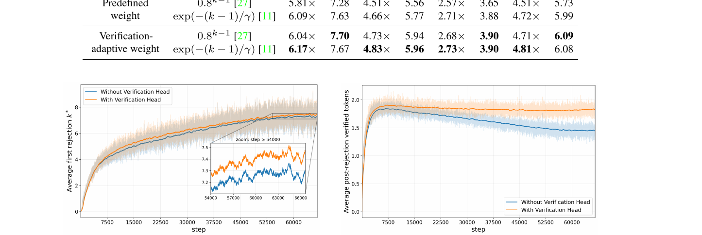
Figure 3 (paper Fig.2, original): Left — average first-rejection position climbs higher (more tokens survive verification) when the verification head is present (orange) versus absent (blue), and the gap widens over training (inset zoom). Right — the number of post-rejection tokens that still coincidentally match the target degrades over training without the head, but stays flat with it, evidence that the head’s gradient is doing real representational work, not just providing a redundant readout.
Component 3: Verification-adaptive weighting
This is the component that directly answers the motivating problem worked through above. VAT replaces the fixed schedule with an instance-adaptive schedule , conditioned on each sample’s own :
Reading this equation carefully: for every position before the first rejection, the weight is simply 1 — full credit, no decay at all, because every such position genuinely contributes to this sample’s acceptance length regardless of how far into the sequence it sits. From onward, VAT reuses the exact same decay function the base method already had ( for EAGLE-3, for DFlash) — but re-indexed to start counting from rather than from . Since both base schedules satisfy , this also means the first-rejection position itself gets full weight — a deliberate design choice, because is “the nearest correctable failure”: it’s exactly where verification actually fails for this sample, so an improved prediction right there directly extends the accepted prefix, making it at least as valuable to get right as any pre- position.
Numbered pseudocode:
Algorithm 2: Verification-adaptive weighting
Input: base schedule function w(.), simulated first-rejection position k*, sequence length K
Output: per-position weights ŵ_1..K

1.  for k = 1 to K:
2.      if k < k*:
3.          ŵ_k <- 1.0                    # full credit, pre-rejection
4.      else:
5.          ŵ_k <- w(k - k* + 1)          # re-anchored decay, starting at k*
6.  return ŵ_1..K
The full combined objective
VAT’s final training objective combines the reweighted, dual soft+hard-label cross-entropy with the verification head loss:
where is cross-entropy against the target’s full output distribution, is cross-entropy against the target’s sampled token, and (set to 1.0 throughout) balances the auxiliary verification-head loss against the reweighted draft loss. The use of both soft and hard labels together (a standard knowledge-distillation combination) is itself a small but real design choice the paper ablates independently: DFlash originally trains with hard labels only, and adding the soft label alone raises from 5.73 to 5.82 in the ablation table, because matching the target’s full distribution (not just its argmax) turns out to carry extra useful signal about the target’s confidence.
Putting it together: the full training-time data flow
flowchart TD
    P["Training batch: prefix + target-generated response"]
    P --> DR["Draft model produces p̂_1..K<br/>(K candidate positions)"]
    P --> TG["Target model produces p_1..K<br/>(same K positions, teacher signal)"]
    DR --> SIM["Algorithm 1: simulate verification<br/>compute m_k, k*, v_k"]
    TG --> SIM
    SIM --> WT["Algorithm 2: verification-adaptive<br/>weighting -> ŵ_k"]
    SIM --> VH["Verification head loss L_VH<br/>(BCE against v_k, Eq.5)"]
    DR --> CE["Reweighted CE loss<br/>Σ ŵ_k (ℓ_soft_k + ℓ_hard_k)"]
    WT --> CE
    CE --> LOSS["Total loss L (Eq.7)"]
    VH --> LOSS
    LOSS --> BP["Backprop into draft model<br/>+ verification head weights only"]
    BP -.->|"target model frozen,<br/>no inference-path changes"| INF["Inference: unchanged SD loop<br/>(optionally: head enables early exit)"]
Figure 6 (self-drawn): The complete VAT training-time data flow — every new component (simulated verification, adaptive weighting, verification head) sits entirely inside the training loop and feeds a single combined loss; nothing here touches the target model’s weights or the inference-time drafting/verification procedure, which is precisely what makes VAT a drop-in addition to an existing pipeline.
Why not simpler alternatives? Design-choice discussion
The paper is unusually thorough about testing alternatives to Eq. (6), which is worth walking through because it clarifies why this particular functional form, rather than something simpler, was chosen (all comparisons on DFlash + Qwen3-4B, 1-epoch budget, Table A in the paper):
- Prefix-only (zero weight from onward, i.e., drop the “decay, don’t eliminate” idea entirely): this collapses below the baseline (speedup 2.44× vs. baseline 4.27×). The failure mode is intuitive once you see the training dynamics in Figure 2: early in training, tends to be small for most samples (the untrained drafter disagrees with the target quickly), so zeroing everything past throws away almost all of the gradient signal exactly when the model needs it most. This tells you decayed-but-nonzero signal past is not optional — it’s load-bearing.
- Hard cutoff (full weight at , then exactly zero after): recovers most of the gap (4.44× vs. VAT’s 4.61×) but still trails VAT, showing that positions past still carry some useful learning signal when decayed rather than eliminated outright — full elimination is still a small amount of wasted information.
- Unshifted decay (apply the base schedule from as usual, i.e., don’t re-anchor at all — effectively “keep the original schedule but don’t otherwise change anything”): 4.46× vs. 4.61×, isolating specifically the value of re-anchoring, independent of the decay function’s shape.
- Marginal-contribution weighting (a more principled-looking alternative: weight each position by the exact derivative of expected acceptance length with respect to that position’s correctness, which naturally discounts positions whose preceding prefix is already uncertain): 4.38× — close to unshifted decay, but still below VAT’s hard -anchoring. The paper’s implicit argument here is that a soft, continuous, confidence-based estimate of “how likely is this position to matter” is a noisier training signal than the hard, ground-truth obtained by actually simulating verification, even though the marginal-contribution scheme is in some sense more theoretically principled.
- GRIFFIN-style masking (zero the loss wherever the drafted token falls outside the target’s top-, a criterion from prior work that is local — evaluated independently per position, not conditioned on prefix survival): 4.32×, the weakest alternative other than prefix-only, reinforcing that a criterion which ignores the sequential all-or-nothing structure of verification (unlike ‘s definition in Eq. 4) systematically under-performs one that respects it.
Where does VAT plausibly still fail, or trade off? The ablation table shows the residual margin between VAT and hard-cutoff/unshifted-decay is real but not huge (roughly 0.15–0.3× speedup), meaning most of the benefit comes specifically from re-anchoring at (the core idea), and the “decay rather than eliminate” refinement past is a smaller, secondary improvement on top. A fair critique is that the paper doesn’t report the standalone re-anchoring-with-hard-cutoff variant combined with the verification head to isolate exactly how much of the total 8–11% acceptance-length gain the weighting scheme itself is responsible for versus the head, though Table 2 (discussed next) does show both factors are individually positive and roughly additive when combined.
A formal look at why acceptance length is the metric to optimize
It’s worth deriving explicitly why (average acceptance length) is not merely “a nice proxy” but the exact quantity that determines end-to-end speedup, since this is the load-bearing assumption behind the entire paper’s motivation. Assume, for simplicity, a fixed per-cycle overhead: one target-model forward pass costs (regardless of how many draft tokens accompany it, since verification of positions in parallel costs about the same as verifying one, as noted in the Prerequisites section above), and one drafting round costs (small, since the draft model is lightweight). If a verification cycle accepts, on average, tokens before hitting a rejection, then generating tokens total requires roughly verification cycles, each costing . Compare this to the non-speculative baseline, which needs target forward passes, each costing . The resulting speedup is:
Two things fall directly out of Eq. (8). First, speedup is linear in , holding the cost ratio fixed — so an 11.4% improvement in should translate to a roughly proportional improvement in speedup, modulo the fact that itself is not perfectly constant across methods (e.g., DFlash’s constant-cost parallel drafting versus EAGLE-3’s -step autoregressive drafting have different profiles, which is part of why the paper’s speedup percentage gains and percentage gains in Table 1 track closely but are not numerically identical — e.g., EAGLE-3 on Qwen3-4B: improves 8.0% but speedup improves 7.9%, an extremely close match consistent with Eq. (8), while DFlash’s larger post-training overhead delta suggests itself changed slightly under VAT training, since DFlash’s early-exit variant explicitly changes how much drafting compute is spent per cycle). Second, and this is the point that most directly justifies training a drafter to maximize rather than, say, per-token accuracy or perplexity: Eq. (8) contains no term at all for how “correct” or “fluent” individual draft tokens are in isolation — only how many of them survive the sequential, all-or-nothing verification process before the first failure. A drafter that produces beautiful, highly plausible tokens that just happen to disagree with the target slightly earlier in the sequence is strictly worse, by this formula, than a drafter that produces slightly blander tokens that happen to survive one position longer. This is precisely the gap between (individual-position correctness) and (survives-the-prefix correctness) formalized in Eq. (4), and it is the single clearest argument for why optimizing directly (via the verification head) and reweighting toward each sample’s own (via Eq. 6) are the theoretically correct things to do, rather than merely convenient engineering hacks.
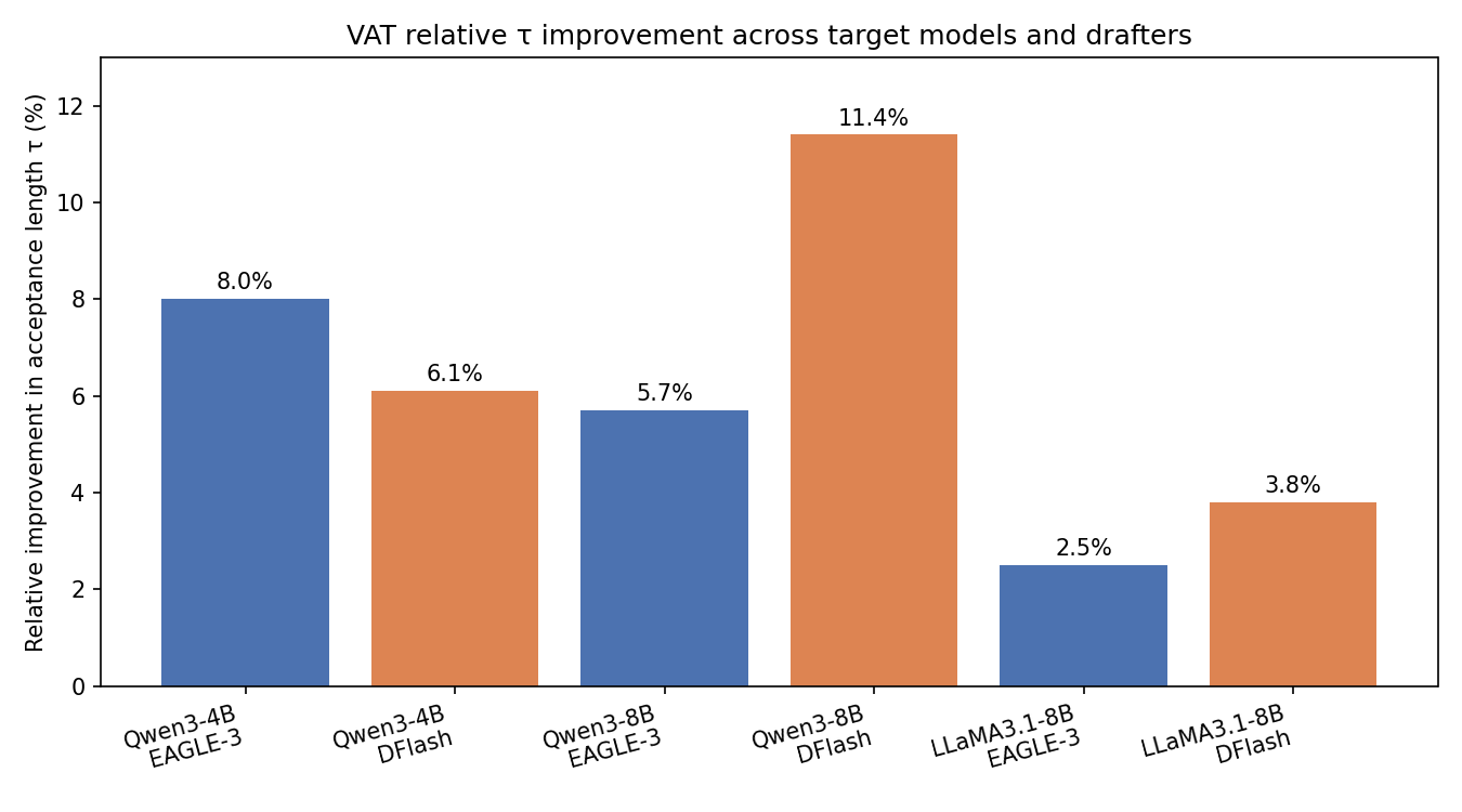
Figure 7 (self-drawn): Plotting the six speedup combinations from Table 1 as relative τ improvement makes the uneven-gain pattern visually obvious — blue bars (EAGLE-3) and orange bars (DFlash) range from 2.5% to 11.4%, and the ranking does not follow a single consistent rule tied purely to baseline strength, as discussed below.
Per-model breakdown: reading the headline numbers carefully
To make the “uneven relative gain across target models” pattern concrete rather than just asserted, here is a compact summary table distilled from the paper’s Table 1 (temperature = 0, averaged over all eight benchmarks):
| Target model | Method | Baseline τ | +VAT τ | Δτ | Baseline speedup | +VAT speedup | Δspeedup |
|---|---|---|---|---|---|---|---|
| Qwen3-4B | EAGLE-3 | 6.28 | 6.78 | +8.0% | 4.07× | 4.39× | +7.9% |
| Qwen3-4B | DFlash | 5.73 | 6.08 | +6.1% | 4.54× | 4.81× | +5.9% |
| Qwen3-8B | EAGLE-3 | 6.12 | 6.47 | +5.7% | 4.04× | 4.24× | +5.0% |
| Qwen3-8B | DFlash | 5.51 | 6.14 | +11.4% | 4.47× | 4.86× | +8.7% |
| LLaMA-3.1-8B | EAGLE-3 | 6.08 | 6.23 | +2.5% | 4.17× | 4.33× | +3.8% |
| LLaMA-3.1-8B | DFlash | 5.57 | 5.78 | +3.8% | 4.08× | 4.22× | +3.4% |
Reading this table row by row surfaces a pattern the paper’s prose doesn’t fully unpack: the largest single gain in the entire table (DFlash on Qwen3-8B, +11.4% τ) belongs to the combination with the lowest baseline τ among the DFlash rows (5.51, versus 5.73 for Qwen3-4B and 5.57 for LLaMA-3.1-8B) — consistent with a “more headroom when baseline acceptance is already weaker” story, though this pattern doesn’t hold cleanly on the EAGLE-3 side, where LLaMA-3.1-8B has the lowest baseline τ (6.08) among EAGLE-3 rows but also the smallest relative gain (+2.5%). This inconsistency between the two drafter families is itself informative: it suggests the size of VAT’s benefit is not simply “inversely proportional to how good the baseline already is,” and is more plausibly tied to some interaction between the target model family’s output distribution shape (Qwen3 vs. LLaMA-3.1 use different tokenizers, different training corpora, and reportedly different confidence calibration behavior) and each drafter architecture’s specific failure modes — a mechanism the paper does not investigate directly, and a natural next experiment for follow-up work (see Critical Analysis below).
Experiments and Results
Setup
VAT is evaluated on top of two structurally different SOTA drafters — autoregressive EAGLE-3 and diffusion-based DFlash — with three target models (Qwen3-4B, Qwen3-8B, LLaMA-3.1-8B-Instruct), across eight benchmarks spanning math (GSM8K, MATH-500, AIME25), code (HumanEval, MBPP, LiveCodeBench), and chat (MT-Bench, Alpaca), using each baseline’s original published hyperparameters (e.g., DFlash’s ) so the comparison is apples-to-apples on top of already-tuned baselines, not against a weakened baseline. Training data pairs PerfectBlend prompts with target-model-generated responses, matching prior work’s recipe.
Headline results
Table 1 in the paper (not reproduced verbatim here for space, but summarized): averaged over all eight benchmarks at temperature 0, EAGLE-3 + VAT improves acceptance length by 8.0% on Qwen3-4B (6.28 → 6.78), 5.7% on Qwen3-8B, and 2.5% on LLaMA-3.1-8B; DFlash + VAT improves by 6.1%, 11.4%, and 3.8% on the same three models respectively. Wall-clock speedup tracks the same pattern: EAGLE-3’s speedup on Qwen3-4B rises from 4.07× to 4.39× (+7.9%), and DFlash’s rises from 4.54× to 4.81× (+5.9%). The gains hold consistently across every one of the 3 models × 2 baselines × 8 benchmarks combinations at both temperature 0 and temperature 1 evaluation — there is no combination in the paper’s tables where VAT makes things worse, which is a meaningfully strong claim for a method this simple.
Two patterns are worth noting in the per-model breakdown. First, the relative gain is uneven across target models — largest on Qwen3-4B and Qwen3-8B, smallest on LLaMA-3.1-8B (2.5–3.8%). The paper doesn’t explicitly explain this gap, but a plausible reading is that Qwen3’s drafters (both baselines) may already have somewhat more headroom for re-weighting to help, given the family’s training data and vocabulary characteristics differ from LLaMA’s — this is worth flagging as underexplained rather than glossing over it, since a reader trying to predict “how much will VAT help my model” cannot straightforwardly extrapolate from these three data points. Second, the paper’s per-benchmark breakdown shows AIME25 (hardest math benchmark) consistently has the smallest absolute gains and even in a couple of cells (e.g., LLaMA-3.1-8B temperature 1) a smaller relative uplift than easier benchmarks — plausibly because harder reasoning has inherently lower drafter/target agreement regardless of training objective, leaving less room for any training-time fix to move .
Ablations that isolate each component’s contribution
Table 2 in the paper (factor analysis, DFlash + Qwen3-4B) shows each of the three ingredients — verification head, verification-adaptive weighting, soft+hard labels — improves on its own (from a 5.73 baseline to 5.87, 5.91, and 5.82 respectively), and combining any two compounds the gain further, with all three together reaching the best result (6.08, +6.1% over baseline). This “each factor helps alone, and they roughly stack” pattern is reassuring evidence against the alternative, less charitable hypothesis that the gains are really coming from just one dominant trick dressed up as three.
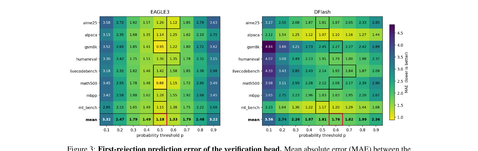
Figure 4 (paper Fig.3, original): Heatmaps of mean absolute error between the target’s true first-rejection position and the verification head’s predicted first-rejection position, per benchmark, as the decision threshold varies from 0.1 to 0.9. The mean row (bottom) is minimized at for EAGLE-3 (MAE 1.18 tokens) and for DFlash (MAE 1.76 tokens) — small enough that the head is a genuinely useful cheap proxy for where verification will actually stop.
A genuinely useful side benefit: early-exit drafting
Because the verification head, once trained, is a cheap forward-pass byproduct that predicts per-position acceptance probability, the paper explores using it at inference time (optionally — it’s not required) to terminate drafting early once a rejection is predicted, rather than always drafting the full tokens and then discovering some were wasted. For DFlash, which drafts all tokens in one parallel pass regardless, “early exit” means sending only the predicted-accept prefix to the target for verification (saving verification compute, not drafting compute). For EAGLE-3, which drafts autoregressively, early exit can also terminate the drafting loop itself, saving both drafting and verification compute.
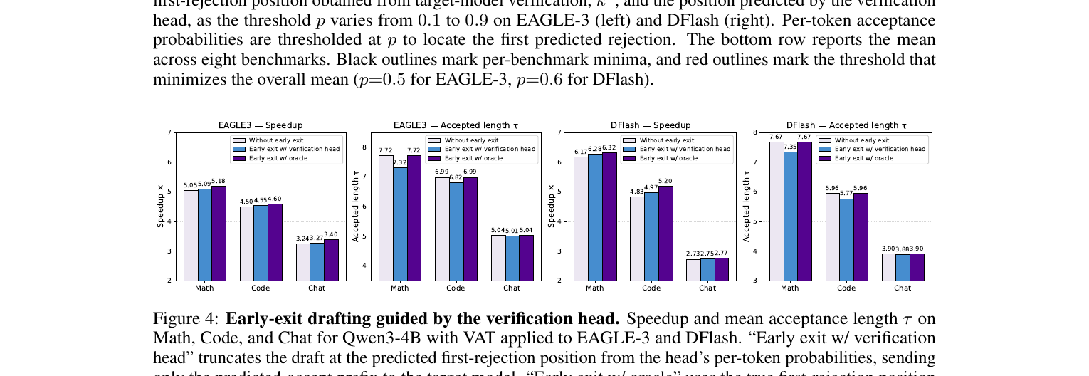
Figure 5 (paper Fig.4, original): “Early exit w/ verification head” (blue) sits between the no-early-exit baseline (white) and an oracle upper bound using the true first-rejection position (purple) — e.g., on DFlash Code, 4.83× → 4.97× vs. an oracle ceiling of 5.20×, with a small, expected drop in acceptance length (7.67 → 7.35 on DFlash Math) from occasional false early rejections. This is a genuinely useful free extra the head buys as a training-time-optional feature, though notably it is the one part of VAT that does touch inference behavior if enabled — everything else is training-only.
Training overhead: the honest cost side of the ledger
Table D in the appendix quantifies the training-time cost directly: VAT adds only 1.2% per-step wall-clock time to EAGLE-3 (0.511s → 0.517s/step) because EAGLE-3 already computes the target’s soft-label distribution for its existing loss, so VAT’s simulated verification reuses that computation almost for free — only the lightweight verification head adds cost. DFlash pays more (0.511s → wait, 1.044s → 1.108s/step, +6.1% time, and a larger memory jump from 23.8GB to 31.5GB peak) because DFlash’s original training never computes the target’s full output distribution at all (it trains on hard labels only), so simulating verification requires an entirely new extra target-model forward pass per training step that DFlash didn’t previously need. This is a legitimate, disclosed cost — not hidden in a footnote — and it’s the kind of detail that matters if you’re deciding whether to adopt VAT: the overhead is asymmetric depending on what your existing training pipeline already computes, and DFlash users should budget for a real (if modest, single-digit-percent) training slowdown, not assume it’s free just because inference is unaffected.
Limitations
The authors are candid about scope limits, and there are a few worth restating and extending:
- Model scale ceiling. All experiments are on target models up to 8B parameters (Qwen3-4B/8B, LLaMA-3.1-8B). The paper explicitly flags scaling to “significantly larger models” as future work. Whether the acceptance-length gains persist, shrink, or grow at 70B+ scale — where drafter/target capacity gaps are typically larger and acceptance rates behave differently — is genuinely unknown from this paper alone.
- Only two drafting paradigms tested. EAGLE-3 (autoregressive, feature-level) and DFlash (block-diffusion, parallel) are both strong, recent baselines, but they don’t cover every architecture family in the SD literature (e.g., Medusa-style independent heads, retrieval-augmented drafters like REST). The claim that VAT is “architecture-agnostic” is plausible given the mechanism (it only touches the loss, not the forward pass), but it is empirically demonstrated on exactly two points in a much larger design space.
- Training corpus dependency. The training set is built by pairing PerfectBlend prompts with target-model-generated responses at greedy decoding, and Appendix B shows robustness to swapping the corpus-generation temperature and verification rule — but this only tests robustness within the paper’s own corpus-construction recipe, not against qualitatively different training-data distributions (e.g., real user traffic logs, adversarial prompts, or domains far from math/code/chat).
- The uneven per-model gain pattern (2.5% to 11.4%) is reported but not explained, as noted above. A method whose benefit varies by nearly 5x across three target models without a stated mechanism for why is harder for a practitioner to reason about a priori than one with a consistent effect size and an explained cause.
Critical Analysis
Weaknesses and flaws specific to this paper. The single most notable gap is the missing ablation connecting verification-adaptive weighting combined with the verification head against the isolated hard-cutoff and unshifted-decay baselines from Table A — Table A only tests weighting variants without the head, so we don’t know whether the ~0.15–0.3x margin VAT’s weighting has over simpler alternatives holds, shrinks, or grows once the head is also present and potentially already captures some of the same “which positions matter” information the weighting redesign targets. There’s a real risk of information redundancy between the two components that the current ablation structure (Table 2 tests presence/absence of each component against the original fixed-weight baseline, not against each other’s near-neighbors) can’t cleanly rule out. Second, the paper reports averages across eight benchmarks in its headline numbers but the per-benchmark tables (Table 1) show real heterogeneity — Alpaca and MT-Bench (chat) consistently show the smallest absolute speedup gains and even occasional near-flat or slightly negative deltas on LLaMA-3.1-8B at temperature 1 (e.g., DFlash: 1.78× → 1.85×, +0.07 in speedup, +0.14 in τ — positive but marginal) — and the paper does not discuss whether chat-style, open-ended generation (where target-drafter disagreement patterns likely differ structurally from math/code, which have more deterministic “correct” continuations) is a systematically harder regime for this class of method.
Limitations the authors understate or omit. The paper frames VAT as broadly “architecture-agnostic,” but this claim rests on a mechanism argument (VAT only touches the loss function) rather than broad empirical coverage — the paper tests exactly two drafter families, both from a fairly narrow “feature-conditioned neural drafter” design space. Methods with fundamentally different training signals — e.g., retrieval-based drafters that don’t produce a full output distribution over the vocabulary at all, or n-gram/lookup-table drafters — would need non-trivial adaptation of Eq. (2)‘s acceptance-probability computation, which assumes access to well-calibrated probability distributions from both models. The paper also doesn’t discuss what happens if the verification rule used during deployment differs from greedy top-1 agreement (e.g., nucleus sampling with a different top-p at inference than was simulated during training) beyond the temperature-1 corpus-generation experiment in Appendix B, which tests corpus generation temperature, not deployment-time sampling policy — these are related but distinct axes, and conflating them slightly overstates how thoroughly the robustness claim has been tested.
Concrete, specific improvement suggestions. (1) Run the missing cross-ablation: verification-adaptive weighting combined with the head, versus hard-cutoff combined with the head, versus unshifted-decay combined with the head — this would directly settle whether the weighting redesign’s benefit is independent of, or partially subsumed by, the head’s contribution. (2) Extend the scaling study to at least one model in the 30–70B range, even with a smaller benchmark subset, since acceptance-length dynamics are known in the broader SD literature to shift non-trivially with target model scale (larger targets tend to have sharper, more peaked distributions, which can change how often saturates at 1). (3) Report a breakdown of where the 2.5%-vs-11.4% variance across target models comes from — e.g., is it correlated with the baseline acceptance length (models that already accept more have less headroom), with tokenizer/vocabulary differences between Qwen3 and LLaMA-3.1, or with something about the training corpus’s coverage of each model family’s typical outputs? Even a correlation-based post-hoc analysis using data the paper already has (Table 1) would meaningfully strengthen the “why does this work when it works” story. (4) For the early-exit inference-time use of the verification head (Figure 4), report end-to-end latency (not just speedup relative to autoregressive decoding) including the extra head forward pass cost, since a reader deciding whether to enable early exit in production needs the full latency accounting, not just the relative-speedup framing used in the paper.
A worked numeric example of the weighting schemes
To make the difference between the fixed schedule, hard cutoff, and VAT’s verification-adaptive weighting completely concrete, consider draft positions under the EAGLE-3-style base schedule , for a single training sample whose simulated first rejection lands at :
| Position | Fixed schedule (Eq. 1) | Hard cutoff | Unshifted decay applied past | VAT (Eq. 6) |
|---|---|---|---|---|
| 1 | 1.00 | 1.00 | 1.00 | |
| 2 | 1.00 | 0.80 | 1.00 | |
| 3 | 1.00 | 0.64 | 1.00 | |
| 4 () | 1.00 | 0.51 | ||
| 5 | 0.00 | 0.41 | ||
| 6 | 0.00 | 0.33 |
Reading across this table row by row makes the paper’s argument tangible. Under the plain fixed schedule, position 3 — which genuinely precedes the rejection and contributes fully to this sample’s accepted prefix — gets discounted to 0.64, identical to what it would get in any sample regardless of where that sample’s own rejection actually lands. VAT instead gives positions 1–3 full weight (they are all pre-), matching the hard-cutoff column exactly up to ; the two methods diverge only from onward, where VAT applies the same decay shape as before but restarts the exponent count from (so position 5, one step past , gets rescaled to the position-2 weight in the re-indexed sequence, i.e. ), whereas hard cutoff simply zeroes those positions outright. This worked example is exactly why the ablation results in Table A make sense qualitatively: hard cutoff and VAT agree on the “don’t discount the pre-rejection prefix” fix, which is where most of the improvement over the fixed schedule comes from, while VAT’s extra edge over hard cutoff comes specifically from the smaller, secondary refinement of keeping some (decayed) signal on positions 5 and 6 rather than discarding them completely.
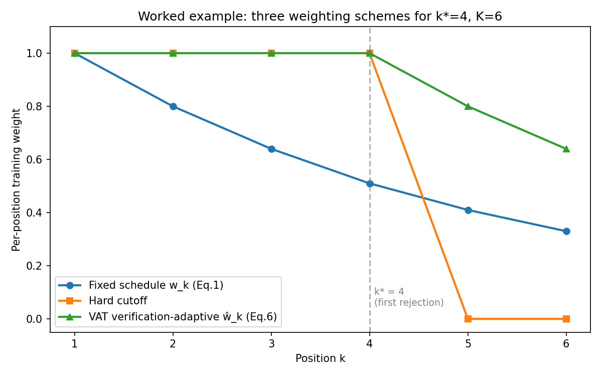
Figure 8 (self-drawn): Plotting the worked-example table above as a line chart makes the qualitative difference between schemes obvious at a glance — the fixed schedule (blue) decays from position 1 onward, discounting positions 2 and 3 even though they are still pre-rejection; hard cutoff (orange) holds full weight up to but zeroes everything after; VAT (green) also holds full weight up to , but keeps decayed (not eliminated) signal past it — the only one of the three that satisfies both “don’t discount the pre-rejection prefix” and “don’t discard all post-rejection signal.”
Broader Context: Where VAT Sits in the Speculative Decoding Landscape
It’s worth situating VAT against the wider families of related work the paper cites but discusses only briefly, since understanding why VAT’s specific combination of ideas is distinct helps clarify what a practitioner gains (and doesn’t gain) by adopting it over alternatives.
Architecture-focused lineage (EAGLE family, Medusa, Hydra, DFlash). The dominant axis of innovation in speculative decoding to date has been drafter architecture: Medusa attaches independent parallel prediction heads directly onto the target’s hidden states (cheap, but heads don’t condition on each other, limiting acceptance length for longer drafts); Hydra adds sequential dependence between those heads (closing some of that gap at added complexity); EAGLE replaces heads entirely with a lightweight autoregressive model operating on the target’s own feature space rather than raw tokens, exploiting the intuition that the target’s hidden state already encodes most of what determines its next-token choice; EAGLE-3 further fuses multi-layer features and exposes the drafter to its own rollouts during training (closing a different mismatch — train/inference mismatch in rollout distribution, not verification-outcome distribution, which is VAT’s target); DFlash abandons autoregressive drafting altogether in favor of block-diffusion parallel generation. VAT is orthogonal to every method in this lineage — it doesn’t propose a new drafter architecture at all, it proposes a new training signal for whatever drafter architecture you already have. This is precisely why the paper can demonstrate compatibility with both an autoregressive drafter (EAGLE-3) and a diffusion drafter (DFlash) without modification: the architectural lineage and the training-objective lineage are genuinely separable axes.
Training-objective lineage (the smaller, more directly comparable body of work). A much smaller set of papers has previously touched the training objective rather than the architecture. DistillSpec examines knowledge distillation between draft and target distributions generally, without reference to the verification-outcome structure. HASS and EAGLE-3’s own training-time test address a related but distinct mismatch: they expose the drafter to sequences generated from its own rollouts during training (rather than always conditioning on ground-truth/teacher-forced prefixes), closing the classic train/inference exposure-bias gap familiar from sequence generation more broadly — but even after this fix, both retain the same uniform, sample-agnostic per-position weighting VAT critiques. Judge Decoding, SpecDec++, and AutoJudge use accept/reject information, but as an inference-time signal (e.g., to decide when to stop drafting or how to weight acceptance decisions at serve time), not as a training-time supervision target — this is an important distinction: VAT’s verification head could plausibly serve a similar inference-time role (and the paper does explore exactly this in its early-exit experiments), but its primary purpose is reshaping training gradients, which is a fundamentally different lever than post-hoc inference-time gating. Two works the paper flags as genuinely concurrent — PARD-2 and D-PACE — are the closest prior art in spirit: both replace fixed positional weighting with adaptive per-position weights. The key technical distinction VAT draws (and it is a real, checkable distinction, not just marketing language) is that PARD-2’s weights derive from the target’s cumulative confidence over the preceding prefix (a soft, probabilistic proxy for “how likely is this prefix to survive”) while D-PACE derives weights from a differentiable surrogate of expected acceptance length based on the draft’s own confidence — both are continuous, confidence-based estimates of importance. VAT instead conditions its weighting on the observed, hard, ground-truth first-rejection position obtained by literally simulating the verification rule, and additionally couples this with the verification head’s explicit supervision of the cumulative outcome , which neither PARD-2 nor D-PACE includes. The ablation study discussed above (Table A) directly tests a D-PACE-style confidence-based weighting inside VAT’s own framework and finds it underperforms the hard-anchored version (4.52×/5.89 vs. VAT’s 4.61×/6.03) — a meaningful, controlled comparison rather than an assumption.
Where this leaves the field. The practical takeaway for a systems engineer choosing between these options: if you already have a working drafter (any architecture) and are looking for a training-time-only improvement with essentially no inference-side cost or risk, VAT’s specific combination — hard -anchored reweighting plus an auxiliary verification head — is currently the most rigorously ablated option in this specific sub-area, per the comparisons the paper itself runs against PARD-2-style and D-PACE-style alternatives within a controlled setting. Whether VAT’s edge over these very recent concurrent methods (PARD-2, D-PACE) holds up under a head-to-head comparison run by an independent third party, on each method’s own preferred hyperparameters rather than reimplemented inside VAT’s framework, remains to be seen — the comparison in Table A, while informative, is necessarily VAT-favorable in its framing (all a la carte weighting schemes are evaluated as drop-in replacements for exactly one piece of VAT’s own pipeline, not as complete competing systems).
Practical Guidance for Adopting VAT
For a reader deciding whether to actually implement this in a production drafter-training pipeline, a few concrete takeaways distilled from the paper’s own numbers:
- The verification-adaptive weighting change (Eq. 6) is the higher-leverage, lower-cost component to adopt first. It requires zero extra forward passes beyond what your existing distillation pipeline already computes (you already have and if you’re doing soft-label distillation), and the ablation in Table A shows it alone accounts for the majority of the gain over any single alternative weighting scheme. If your training pipeline is compute-constrained, start here.
- The verification head is cheap for EAGLE-3-style pipelines (1.2% overhead) but meaningfully more expensive for DFlash-style pipelines (6.1% overhead, plus a ~32% peak memory increase) because it requires an entirely new target-model LM-head pass that DFlash’s original recipe never computed. If you’re training a diffusion-style drafter and are memory-constrained, budget for this explicitly before committing.
- The early-exit inference-time use of the verification head is a genuinely separate decision from adopting VAT for training. You can adopt VAT purely for its training-time benefit (better with unchanged inference) without ever touching early exit, or you can additionally enable early exit for a further speedup at the cost of a small reduction from occasional false-rejection predictions (Figure 5/6 above). These are two independent knobs, not a package deal.
- Sensitivity to target model choice is real and currently unexplained (Section “Per-model breakdown” above) — if your target model differs substantially from Qwen3 or LLaMA-3.1 (e.g., a different tokenizer, a mixture-of-experts architecture, or a much smaller/larger parameter count), treat the reported 2.5–11.4% range as a plausible envelope rather than a guaranteed outcome, and budget time for your own ablation before assuming a specific number transfers.
Reproducibility Notes
The paper states code “will be available” at https://github.com/naver-ai/VAT (not yet public as of this review’s writing), and explicitly builds on two already-open baselines — EAGLE-3 (https://github.com/SafeAILab/EAGLE) and DFlash (https://github.com/z-lab/dflash) — which substantially lowers the reproduction bar once VAT’s own code lands, since a reader can start from either baseline’s existing training pipeline and layer in Eq. (6)‘s re-anchored weighting and Eq. (5)‘s verification head, both of which are simple enough (a handful of lines: compute from the existing target/draft distributions already used for the soft-label loss, re-index the existing decay function, add one dense layer plus a BCE term) to plausibly reimplement from the paper’s equations alone even before the official code is released. The paper reports all training on A100 80GB GPUs, 3 epochs, standard hyperparameters copied from the original EAGLE-3/DFlash papers (with for DFlash’s decay explicitly stated), and provides a full training-overhead table (Table D) with concrete per-step timing and memory numbers, which is unusually good practice for helping a re-implementer sanity-check their own numbers against the paper’s reported training cost.