RRC: Unlocking Generative Reward Models in LLM Reinforcement Learning via Ranking-Based Reward Construction

Review date: 2026-09-01 Paper reviewed: RRC: Unlocking Generative Reward Models in LLM Reinforcement Learning via Ranking-Based Reward Construction Paper authors: Chenglong Wang, Ziming Zhu, Yifu Huo, Bei Li, Qiaozhi He, Yan Ding, Xiaoyang Hao, Yuxin Gao, Tianhua Zhou, Xiaojia Chang, Tongran Liu, Jingbo Zhu, Zhengtao Yu, Tong Xiao (Northeastern University / NiuTrans Research / CAS Institute of Psychology / Kunming University of Science and Technology) arXiv: 2608.06310 Venue/Status: arXiv preprint, submitted 6 Aug 2026

1. What Problem Is This Paper Actually Solving?

Every RLHF or RLVR-style pipeline for LLMs needs a reward signal. For a long time, that signal came from discriminative reward models (DRMs): take a pretrained LLM backbone, strip its output head, and replace it with a linear layer that spits out a single scalar number for a given (prompt, response) pair. Simple, fast, and battle-tested — but it throws away most of what made the backbone useful in the first place, namely its ability to generate text and reason in natural language.

Generative reward models (GRMs) try to keep that ability. Instead of collapsing straight to a number, a GRM is prompted with a pair of candidate responses and asked to write out a judgment — optionally with explicit chain-of-thought (CoT) reasoning — before naming which response is better. On pure pairwise-ranking benchmarks (RM-Bench, JudgeBench), GRMs beat DRMs by a wide margin: this paper reports +7.5% on RM-Bench and +4.2% on JudgeBench for the same backbone and the same training data. GRMs are, empirically, better judges.

So here is the puzzle the paper opens with: if GRMs are so much better at judging, why does swapping a DRM for a GRM inside an RL loop (GRPO, PPO, DAPO, …) produce only a marginal improvement — sometimes within noise — in the trained policy’s downstream quality? The paper’s own replication (their Figure 1(b)) shows RL-with-GRM beating RL-with-DRM by only +1.3% on AlpacaEval2, a small fraction of the ranking-side advantage.

The paper’s diagnosis is architectural, not just a training-recipe quirk: existing RL algorithms want a scalar reward per response, and the standard way of extracting a scalar from a GRM is fundamentally mismatched with what a GRM is good at. The common trick (used by GenRM, GRAM, and similar prior work) is to prompt the GRM with a reference response $o_{\text{ref}}$ alongside the candidate $o$, and read off the softmax probability that the model assigns to the token indicating ”$o$ is preferred” — treating that probability as if it were a calibrated scalar reward. The paper shows this probability-based construction has two concrete failure modes:

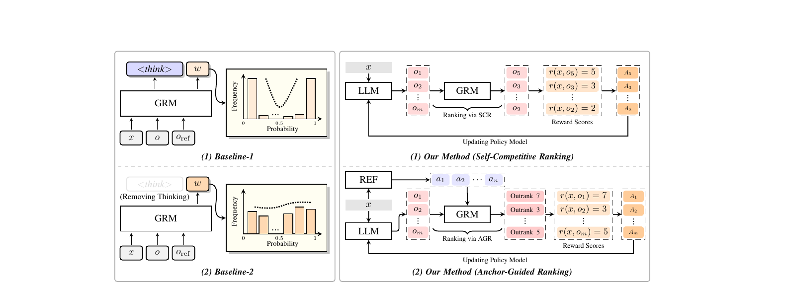
1. Probability collapse under CoT. When the GRM is allowed to reason before answering, its final preference token probability tends to saturate near 0 or 1 (the paper measures this directly — see §6 below, Table 6 in the appendix: 88.3% of samples fall in the extreme buckets $[0,0.1]\cup[0.9,1.0]$, only 11.7% in the informative middle range). A near-binary reward gives almost no gradient signal to distinguish a slightly better response from a dramatically better one.
2. Confidence $\ne$ preference strength. Even when the probability isn’t saturated, it reflects the model’s confidence in its own judgment call, which is a different quantity from the actual quality gap between the two responses, and can simply be noise.

RRC’s proposed fix is conceptually blunt but effective: stop asking GRMs to produce scalar scores at all. Use them only for what they’re demonstrably good at — pairwise comparative judgments — and construct the scalar reward that RL needs after the fact, from the structure of many such pairwise comparisons (via win-counting and ranking aggregation), rather than from a single probability read out of the model’s own uncertainty.

2. Prerequisites: What You Need to Understand First

2.1 Reward models: discriminative vs. generative, in more detail

A reward model is a function $r_\phi(x, y)$ that assigns a score to a response $y$ given input $x$. There are exactly two architectural families in production use today.

Discriminative reward models. Built on a Transformer backbone (encoder-only, or a decoder with the softmax head removed and replaced by a linear projection). The final-layer hidden state of the concatenated $(x,y)$ sequence is mapped to a single scalar via a linear layer. Training uses the Bradley-Terry model (Bradley & Terry, 1952), a classical statistical model for pairwise comparisons, via the loss

$$\mathcal{L}_d = -\mathbb{E}_{(x,y_a,y_b)\sim D_r}\Big[\log\big(\sigma(r_\phi(x,y_a) - r_\phi(x,y_b))\big)\Big], \tag{1}$$

where $D_r$ is a preference dataset of tuples with $y_a \succ y_b$ (i.e., $y_a$ is preferred), and $\sigma$ is the logistic sigmoid. Intuitively, this loss pushes the difference of the two scalar scores through a sigmoid and asks that difference to predict the preference — exactly analogous to logistic regression on paired comparisons. Once trained, $r_\phi(x,y)$ can be called directly to get a number for any single response; that number is designed from the ground up to be comparable across different response pairs, because the training loss only ever sees relative differences and the model must learn a globally consistent scale.

Generative reward models. Instead of a scalar head, a GRM uses the LLM’s own generation capability. Given a natural-language instruction prompt $c$ describing the judging task, and a tuple $(x, y_a, y_b)$, the GRM predicts a preference token $w \in \{A, B\}$ indicating which response is better, optionally after writing out a free-text chain-of-thought first. Training uses a straightforward next-token cross-entropy objective on the label token:

$$\mathcal{L}_g = -\mathbb{E}_{(c,x,y_a,y_b,l)\sim D_r}\Big[\log \pi_\phi(w=l \mid s)\Big], \qquad s = [c, x, y_a, y_b], \tag{2}$$

where $l\in\{A,B\}$ is the ground-truth preference label. Notice the crucial structural difference from Eq. (1): the GRM’s training signal is only ever conditioned on a pair — it never sees a single response in isolation, and it never learns to assign that response an absolute number. Everything the GRM knows how to do is comparative. This is the root of the entire paper’s argument, so it’s worth sitting with: a GRM’s “vocabulary” is literally “A or B”, not “a number between 0 and 1 that means something on its own.”

2.2 How RL for LLMs consumes reward

The policy optimization objective in RLHF/RLVR is

$$\max_\theta\; \mathbb{E}_{x\sim D,\, o\sim \pi_\theta(\cdot\mid x)}\big[r_\phi(x, o)\big]. \tag{3}$$

PPO (Schulman et al., 2017) optimizes this with a learned critic that estimates advantages, but the critic itself is expensive and prone to instability. GRPO (Shao et al., 2024) — the workhorse behind DeepSeekMath and DeepSeek-R1-style training, and the algorithm RRC plugs into — removes the critic entirely. It samples a group of $m$ responses $\{o_1,\dots,o_m\}$ for the same prompt $x$ from the current policy, and defines each response’s advantage as its group-normalized reward:

$$A_i^{(r)} = \frac{r_i - \mu_r}{\sigma_r}, \qquad r_i \triangleq r_\phi(x, o_i), \qquad \mu_r \triangleq \frac{1}{m}\sum_{k=1}^m r_k, \qquad \sigma_r^2 \triangleq \frac{1}{m}\sum_{k=1}^m (r_k - \mu_r)^2. \tag{4}$$

This is the load-bearing detail for the rest of the paper: GRPO needs a scalar $r_i$ for every single sampled response so it can compute a group mean and standard deviation. A DRM hands this over for free — it was trained to output exactly that. A GRM was never trained to output a number at all; something has to manufacture one.

2.3 The existing (flawed) bridge: probability-based reward construction

The standard trick to force a GRM into this role: pick a reference response $o_{\text{ref}}$ (typically the greedy decode $\arg\max_o \pi_\theta(o\mid x)$ of the current policy), concatenate $(c, x, o, o_{\text{ref}})$ into a single judging prompt $s_o$, and define

$$r_\phi(x,o) = \pi_\phi(w = A \mid s_o), \tag{5}$$

i.e. the model’s predicted probability that the candidate $o$ (labeled “Response A” in the prompt) is preferred over the reference. This is exactly the mechanism used by GenRM (Zhang et al., 2024) and referenced implicitly by GRAM (Wang et al., 2025b). It’s a reasonable-sounding hack — it does produce a number in $[0,1]$ — but it silently smuggles in an assumption the GRM’s training never actually enforced: that this probability behaves like a well-calibrated, comparable-across-responses scalar score. Section 3 of the paper (and its own Figure 1/Table 6) is a systematic demonstration that this assumption fails.

3. The Diagnostic Experiment: Ranking vs. Scoring (§3 of the paper)

Before proposing a fix, the authors run a controlled comparison. They train a DRM and a GRM on the same LLaMA-3.2-3B-Instruct backbone and the same HelpSteer3 preference data (40.5K examples with human-written rationales, used as CoT supervision for the GRM). They then evaluate both models in two very different settings:

• Response ranking: RM-Bench and JudgeBench — standard pairwise-judging accuracy benchmarks.
• RL: reward scores constructed from predicted preference-token probabilities (Eq. 5), plugged into GRPO, evaluated on AlpacaEval2 win-rate over training steps.

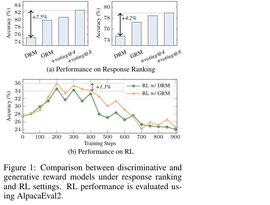
The result is the paper’s entire motivating tension in one figure: on response ranking, the GRM crushes the DRM (+7.5% on RM-Bench, +4.2% on JudgeBench, and majority voting pushes the gap even wider). But when the same GRM is dropped into RL via probability-based reward construction, its advantage over the DRM collapses to +1.3% on AlpacaEval2 — and note in panel (b) that this gap is not even monotonic across training; RL-w/-GRM and RL-w/-DRM cross over repeatedly, and both curves degrade substantially after step ~400, which the paper doesn’t dwell on but is itself a signal that probability-based rewards are noisy learning targets.

Why this happens, mechanically. Go back to Eq. (5). The GRM is asked to output a single probability $\pi_\phi(w=A\mid s_o)$ for a single pairwise comparison $(o, o_{\text{ref}})$. Two things go wrong:

• If the GRM reasons explicitly (writes a CoT before naming a winner), the paper observes that the final preference-token probability tends to saturate: once the CoT has “talked itself into” a conclusion, the softmax over $\{A,B\}$ collapses toward 0 or 1, almost regardless of how close the two responses actually are in quality. A near-deterministic 0.97 vs. 0.99 carries essentially the same gradient information as 0.97 vs. 0.60 once it’s normalized within a GRPO group — the ordering survives, but the margin is destroyed.
• Even when not saturated, the probability reflects epistemic confidence in the judgment, not the latent quality gap between the responses. A GRM might be 60% confident about a genuinely huge quality gap (if the comparison is subtle to articulate) or 95% confident about a tiny one (if one response has an obvious surface-level flaw). Using confidence as if it were quality is a category error.

This sets up exactly the two properties the paper will demand of any fix (§4.1, formalized next).

4. Desiderata for Reward Construction (§4.1)

The paper states two properties any reward function $r(x,o)$ needs to satisfy to be useful for RL, and it’s worth internalizing both precisely because RRC’s entire design is a direct, mechanical satisfaction of them.

Property 1 (Order preservation). For any two responses $(o_i, o_j)$ sampled under the same input $x$: $o_i \succ o_j \implies r(x,o_i) > r(x,o_j)$.

This is the weaker property — it just says the reward function shouldn’t invert the ground-truth preference ordering. Almost any sane reward construction satisfies this trivially.

Property 2 (Margin awareness). The reward difference should track the latent oracle preference margin:

$$r(x,o_i) - r(x,o_j) \propto \Delta q_{ij}, \qquad \Delta q_{ij} \triangleq q(x,o_i) - q(x,o_j), \tag{6}$$

where $q(x,o)$ is an unobservable “oracle” quality function representing the true preference intensity. This is the property that probability-based construction violates under saturation: two very different quality gaps get mapped to the same (saturated) probability difference, destroying the proportionality even while the ordering survives.

4.1 Why margin awareness matters: a policy-gradient argument (full derivation, paper’s Appendix A)

This is presented informally in the main text but proven rigorously in Appendix A; I found it worth walking through in full because it’s the paper’s actual theoretical payload, and most readers will skim past a one-line “we show this matters for RL” without seeing why.

Define the ideal RL objective using the oracle quality function directly:

$$J_q(\theta) \triangleq \mathbb{E}_{x\sim D,\, o\sim\pi_\theta(\cdot\mid x)}\big[q(x,o)\big]. \tag{7}$$

By the policy gradient theorem,

$$\nabla_\theta J_q(\theta) = \mathbb{E}_{x,o}\big[q(x,o)\,\nabla_\theta \log \pi_\theta(o\mid x)\big]. \tag{8}$$

In practice, GRPO-style algorithms estimate this with a sampled group $\{o_1,\dots,o_m\}$ and the group-normalized advantage from Eq. (4). Ignoring PPO-style clipping for clarity, the resulting update direction is

$$g_r(\theta) \triangleq \mathbb{E}_x\Big[\sum_{i=1}^m A_i^{(r)}\,\nabla_\theta \log \pi_\theta(o_i\mid x)\Big]. \tag{9}$$

Step 1 — set up the affine-transform assumption. Suppose the practical reward function $r$ is an affine (i.e. linear plus offset) transform of the oracle quality, for some fixed $x$:

$$r(x,o) = b\, q(x,o) + d, \qquad b > 0. \tag{10}$$

This is the weakest possible condition under which we’d hope $r$ still “does the right thing” relative to $q$ — it says $r$ preserves quality differences up to a constant positive rescaling and shift, which is exactly what margin awareness (Eq. 6, with proportionality constant $b$) asks for.

Step 2 — show group normalization cancels the affine nuisance parameters. Define the analogous group statistics for the oracle quality: $q_i \triangleq q(x,o_i)$, $\mu_q \triangleq \frac1m\sum_k q_k$, $\sigma_q^2 \triangleq \frac1m\sum_k (q_k-\mu_q)^2$. Under the affine assumption (Eq. 10):

$$\mu_r = \frac1m\sum_{k=1}^m (b q_k + d) = b\mu_q + d, \tag{11}$$ $$\sigma_r^2 = \frac1m\sum_{k=1}^m \big(b q_k + d - (b\mu_q+d)\big)^2 = \frac1m\sum_{k=1}^m \big(b(q_k-\mu_q)\big)^2 = b^2 \sigma_q^2 \;\;\Rightarrow\;\; \sigma_r = b\sigma_q \; (\text{since } b>0). \tag{12}$$

Substituting these into the group-normalized advantage (Eq. 4):

$$A_i^{(r)} = \frac{r_i - \mu_r}{\sigma_r} = \frac{(bq_i + d) - (b\mu_q + d)}{b\sigma_q} = \frac{b(q_i - \mu_q)}{b\sigma_q} = \frac{q_i - \mu_q}{\sigma_q} = A_i^{(q)}. \tag{13}$$

This is the crux of the whole derivation: the offset $d$ and the positive scale $b$ cancel exactly under group normalization. In other words, GRPO’s normalized advantage is invariant to any affine transformation of the reward — as long as the affine map is faithful (Property 2 with a constant proportionality factor $b$ that doesn’t itself vary across responses).

Step 3 — conclude: affine-faithful rewards recover the oracle gradient exactly. Substituting $A_i^{(r)} = A_i^{(q)}$ back into the update direction (Eq. 9):

$$g_r(\theta) = \mathbb{E}_x\Big[\sum_{i=1}^m A_i^{(q)}\,\nabla_\theta \log \pi_\theta(o_i\mid x)\Big], \tag{14}$$

which is precisely the group-normalized estimator of the oracle policy gradient (Eq. 8). The practical reward function $r$, despite being an unknown affine transform of $q$, induces the exact same RL update as if you had access to the ground-truth oracle quality.

Step 4 — what happens when margin awareness fails. The contrapositive is the important takeaway: if $r$ is not affine-faithful to $q$ — e.g. if it saturates near the boundary of $[0,1]$ as with probability-based construction — then the induced $A_i^{(r)}$ will not equal $A_i^{(q)}$ for every group, and the relative weighting of the policy-gradient terms across responses will systematically diverge from what the oracle gradient would assign. Concretely: a probability-based reward that’s compressed at the extremes will under-weight updates on response pairs with large genuine quality gaps (because their observed reward gap is artificially small after saturation) and can even over-weight pairs with small genuine gaps that happen to land in the un-saturated middle of the probability range. This is a formal way of saying “the RL signal gets systematically distorted,” not just “noisy” — the distortion has a direction, and it’s a direction the paper’s diagnostic experiment (Figure 1b) is consistent with.

Design-choice note: this derivation only requires $r$ to be affine in $q$ with a response-independent $b$ and $d$ for a fixed prompt $x$ — it does not require $r$ to be affine across different prompts, or to know the absolute scale of $q$ at all. This is a deliberately weak, achievable requirement, and it’s exactly the target RRC’s ranking-based construction is designed to hit (shown in §5 below), whereas probability-based construction fails it because saturation makes the effective "$b$" implicitly response-dependent (it shrinks toward zero near the boundaries of the probability simplex).

5. RRC: Ranking-Based Reward Construction (§4.2)

RRC’s core move: never ask the GRM for a probability at all. Only ever ask it for a pairwise preference judgment — “is $o_i$ better than $o_j$, yes or no” — and build the scalar reward by counting wins across many such judgments. It has two variants that trade off cost against comparison structure.

5.1 Self-Competitive Ranking (SCR)

Idea in one sentence: treat the $m$ responses sampled for the same prompt as mutual competitors, run all $\binom{m}{2}$ pairwise comparisons between them, and reward each response by how many of its comparisons it won.

For each pair $(o_i, o_j)$ in the sampled group, query the GRM for a preference relation:

$$o_i \succ o_j \quad \text{or} \quad o_j \succ o_i. \tag{15}$$

These pairwise judgments induce a tournament graph over the response set (a complete directed graph where each edge points from winner to loser). The reward for response $o_i$ is its win count, scaled by a constant $\alpha$:

$$r(x, o_i) = \alpha \times \sum_{j\ne i} \mathbb{1}[o_i \succ o_j]. \tag{16}$$

Why win-counting satisfies both desiderata. Order preservation (Property 1) is immediate: a response that’s genuinely better than more of its competitors will win more of its pairwise comparisons and get a strictly higher win count, so long as the pairwise judge itself is order-preserving (which — being a well-trained GRM — it should be, at least in expectation). Margin awareness (Property 2) is the more interesting claim, and the paper proves it directly:

$$r_i - r_j = \alpha \sum_k \big(\mathbb{1}[o_i \succ o_k] - \mathbb{1}[o_j \succ o_k]\big). \tag{17}$$

This is the net number of wins of $o_i$ over the rest of the group relative to $o_j$. If $o_i$ is substantially better than $o_j$, then intuitively $o_i$ will tend to beat competitors that $o_j$ loses to — widening the win-count gap. If $o_i$ and $o_j$ are close in quality, their win counts against the rest of the group will also tend to be close. Crucially, this margin emerges without ever asking the GRM to introspect on how confident it is — it’s aggregated from many independent binary decisions, which is exactly the kind of task the GRM’s training objective (Eq. 2) actually optimizes it for.

Complexity. SCR requires all $\binom{m}{2} = \frac{m(m-1)}{2} = O(m\log m)$-ish pairwise queries (the paper writes $O(m\log m)$ loosely, though the exact count is quadratic $O(m^2)$; more on this notational looseness in the Critical Analysis section below).

5.2 Majority Voting for Robust Ranking

A single pairwise call to a GRM is a stochastic sample — especially when explicit CoT reasoning is involved, the model’s chain of thought can wander to different conclusions on repeated queries with the same inputs. RRC stabilizes this with majority voting: for each pair $(o_i, o_j)$, query the GRM $V$ times independently and take the majority-vote winner as the final preference. This trades additional inference-time compute (which the paper frames explicitly as a form of test-time scaling, in the spirit of Muennighoff et al.’s s1) for lower-variance pairwise judgments.

5.3 Conflict-Aware Ranking Adjustment (CARA) — Kemeny-rule aggregation

Pairwise preferences from independently-queried comparisons are not guaranteed to be globally consistent. Cyclic inconsistencies can arise:

$$o_i \succ o_j,\quad o_j \succ o_k, \quad \text{but} \quad o_k \succ o_i, \tag{18}$$

which violates transitivity — you can’t build a single total order (a ranking) out of a preference graph that has cycles. RRC resolves this via a Kemeny-rule-based aggregation — a classical social-choice-theory tool for turning inconsistent pairwise votes into the “least-wrong” consistent ranking.

Property 3 (proved in Appendix A, walked through here). Given inconsistent pairwise preferences with support weights $w_{ij}$ (e.g. the vote count in favor of $o_i \succ o_j$ from majority voting), a Kemeny-rule aggregation recovers a globally consistent total order that maximizes weighted agreement with all pairwise preferences.

Proof walkthrough. Model the response set as a weighted directed graph $G=(V,E)$ with $V=O$, and a directed edge $i\to j$ of weight $w_{ij}$ for every observed preference $o_i \succ o_j$. A total order $\pi$ over $O$ “agrees” with an edge $i\to j$ if $\pi$ ranks $i$ ahead of $j$. Define the weighted agreement and disagreement of $\pi$:

$$\text{Agree}(\pi) := \sum_{i \prec_\pi j} w_{ij}, \qquad \text{Disagree}(\pi) := \sum_{i \prec_\pi j} w_{ji}. \tag{19}$$

Because for any unordered pair $\{i,j\}$ exactly one of $i\prec_\pi j$ or $j\prec_\pi i$ holds under a total order, and every pair contributes exactly $w_{ij}+w_{ji}$ to the sum regardless of $\pi$:

$$\text{Agree}(\pi) + \text{Disagree}(\pi) = \sum_{i<j}(w_{ij}+w_{ji}) =: C, \quad \text{a constant independent of } \pi. \tag{20}$$

Hence $\arg\max_\pi \text{Agree}(\pi) = \arg\min_\pi \text{Disagree}(\pi)$: maximizing agreement and minimizing disagreement are literally the same optimization problem. This is precisely the classical Kemeny-optimal aggregation objective in its weighted form — minimize the total weight of pairwise disagreements, equivalently find the minimum weight feedback edge set whose removal makes the graph acyclic. Because the optimizer $\pi^*$ is by construction a total order, it is trivially transitively consistent (if $i\prec_{\pi^*} j$ and $j\prec_{\pi^*}k$ then necessarily $i\prec_{\pi^*}k$), closing the proof.

Practical algorithm. Exact Kemeny aggregation is NP-hard in general, so RRC uses the greedy heuristic of Davenport & Kalagnanam (2004): repeatedly pick the unresolved pair $(i,j)$ with the largest weight imbalance $|w_{ij}-w_{ji}|$, fix its order according to the majority direction, and maintain acyclicity via transitive-closure propagation as relations are added (i.e., reject any newly proposed relation that would create a cycle with already-fixed relations). The final reward assigned to each response after CARA is its position in the resulting total order $\pi$, converted to a win count:

$$r(x,o_i) \leftarrow \alpha \cdot \big|\{o_j \ne o_i : i \prec_\pi j\}\big|. \tag{21}$$

5.4 SCR’s full algorithm, as numbered pseudocode

The paper’s Algorithm 1 (I’ve reproduced it faithfully, expanding a couple of steps for clarity):

Algorithm 1: Self-Competitive Ranking (SCR) with Majority Voting and CARA
Require: prompt x; responses O = {o_1, ..., o_m}; GRM;
         voting budget V; scaling factor alpha; flag use_CARA
Ensure:  rewards {r(x, o_i)}_{i=1}^m; total order pi

 1: initialize w[i][j] <- 0 for all i != j
 2: for each unordered pair {i, j} with i < j:
 3:     c_ij <- 0   // votes for o_i > o_j
 4:     c_ji <- 0   // votes for o_j > o_i
 5:     for t = 1 to V:
 6:         query GRM on (x, o_i, o_j) -> preference
 7:         if o_i > o_j:  c_ij <- c_ij + 1
 8:         else:          c_ji <- c_ji + 1
 9:     if c_ij >= c_ji:
10:         w[i][j] <- c_ij ; w[j][i] <- c_ji
11:     else:
12:         w[j][i] <- c_ji ; w[i][j] <- c_ij
13: if use_CARA:
14:     initialize partial order Omega <- empty set
15:     while exists undecided pair (i, j):
16:         select (i, j) maximizing |w[i][j] - w[j][i]|
17:         if w[i][j] >= w[j][i]: add relation "i before j" to Omega
18:         else:                  add relation "j before i" to Omega
19:         enforce transitive closure; discard any relation forming a cycle
20:     pi <- topological sort of Omega
21: else:
22:     pi <- sort responses by descending win count sum_j 1[w[i][j] > w[j][i]]
23: for each o_i in O:
24:     r(x, o_i) <- alpha * |{o_j != o_i : i comes before j in pi}|
25: return {r(x, o_i)}_{i=1}^m, pi

Walking through it in prose: lines 2-12 exhaustively query every pair, aggregating $V$ stochastic votes into a majority-decided directed weight for that pair. Lines 13-20 are the optional CARA step — resolve conflicts greedily by fixing the most confident (largest weight-imbalance) pairs first, and refuse any relation that would introduce a cycle given what’s already been fixed. Lines 22-24 convert whichever ranking resulted (CARA’s topological order, or the simple win-count fallback) into the final scalar rewards.

5.5 Anchor-Guided Ranking (AGR)

SCR’s $O(m^2)$ query cost becomes prohibitive as the sampled group size $m$ grows — and larger $m$ is exactly what modern RL recipes want, for better exploration and gradient estimate stability. AGR fixes the scaling problem by replacing all-pairs comparison with comparison against a small, fixed set of anchor responses.

Given a small anchor set $\{a_1,\dots,a_n\}$ ($n \ll m$ in practice), generated by a reference policy $\pi_{\text{ref}}$ (not the current policy — this distinction matters, see §5.6 below), each sampled response $o_i$ is compared against every anchor:

$$r(x, o_i) = \alpha \times \sum_{k=1}^n \mathbb{1}[o_i \succ a_k]. \tag{22}$$

The margin-awareness argument is structurally identical to SCR’s (Eq. 17), just with the anchor set playing the role of “the rest of the group”:

$$r_i - r_j = \alpha \sum_{k=1}^n \big(\mathbb{1}[o_i \succ a_k] - \mathbb{1}[o_j \succ a_k]\big). \tag{23}$$

If $o_i$ reliably outperforms anchors that $o_j$ fails against, the reward gap widens — this time measuring “how much better than a common, fixed yardstick” rather than “how much better than the current competitive field.”

5.6 AGR’s full algorithm, as numbered pseudocode

Algorithm 2: Anchor-Guided Ranking (AGR) with Majority Voting
Require: prompt x; responses O = {o_1, ..., o_m}; anchors A = {a_1, ..., a_n};
         GRM; voting budget V; scaling factor alpha
Ensure:  rewards {r(x, o_i)}_{i=1}^m

 1: for each response o_i in O:
 2:     s_i <- 0
 3:     for each anchor a_k in A:
 4:         c_ik <- 0   // votes for o_i > a_k
 5:         c_ki <- 0   // votes for a_k > o_i
 6:         for t = 1 to V:
 7:             query GRM on (x, o_i, a_k) -> preference
 8:             if o_i > a_k:  c_ik <- c_ik + 1
 9:             else:          c_ki <- c_ki + 1
10:         if c_ik >= c_ki:
11:             s_i <- s_i + 1
12:     r(x, o_i) <- alpha * s_i
13: rank responses by descending r(x, o_i)
14: return {r(x, o_i)}_{i=1}^m

5.7 Design choice: why reference-policy anchors, not on-policy anchors? (Property 3, full derivation)

This is arguably the most subtle design decision in the paper, and it gets a dedicated proof in Appendix A. The naive alternative is to draw anchors from the current policy $\pi_\theta$ itself (e.g., a subset of the same sampled group). RRC deliberately rejects this in favor of anchors drawn from a fixed reference policy $\pi_{\text{ref}}$, independent of the parameters being trained.

Why this matters, mechanically. Write the reward for a response $o_i \sim \pi_\theta(\cdot\mid x)$ under AGR, making the anchor-generating distribution’s dependence on $\theta$ explicit:

$$r_\theta(x, o_i) = \alpha \sum_{k=1}^n \mathbb{1}[o_i \succ a_k], \qquad a_k \sim q_\theta(\cdot\mid x). \tag{24}$$

The full gradient of the RL objective with respect to $\theta$ has to account for both how $\theta$ affects the distribution of sampled responses, and — if anchors also depend on $\theta$ — how $\theta$ affects the anchors used to score them:

$$\nabla_\theta J(\theta) = \underbrace{\mathbb{E}_{x,o}\big[r_\theta(x,o)\,\nabla_\theta \log\pi_\theta(o\mid x)\big]}_{\text{policy improvement term}} + \underbrace{\mathbb{E}_{x,o}\big[\nabla_\theta r_\theta(x,o)\big]}_{\text{baseline drift term}}. \tag{25}$$

Case A — on-policy anchors ($q_\theta = \pi_\theta$). The second term is non-zero:

$$\nabla_\theta r_\theta(x,o) = \alpha \sum_{k=1}^n \mathbb{E}_{a_k\sim\pi_\theta}\big[\mathbb{1}[o\succ a_k]\,\nabla_\theta\log\pi_\theta(a_k\mid x)\big]. \tag{26}$$

Every policy update simultaneously (1) shifts probability mass toward better responses $o$, and (2) improves the anchor set used as the comparison yardstick, since the anchors themselves are drawn from the improving policy. This creates exactly the moving-target problem: as training progresses, $\theta_t \Rightarrow \pi_{\theta_t} \Rightarrow$ stronger anchors $\Rightarrow$ shifted rewards $\Rightarrow \nabla_\theta J(\theta_t)$ changes for reasons unrelated to actual policy quality. This violates the stationarity assumptions that make stochastic gradient ascent well-behaved, and it inflates gradient variance.

Case B — reference-policy anchors ($q_\theta = \pi_{\text{ref}}$, independent of $\theta$). Now $\nabla_\theta r_\theta(x,o) = 0$ identically, and the gradient collapses to just the policy-improvement term:

$$\nabla_\theta J(\theta) = \mathbb{E}\big[r(x,o)\,\nabla_\theta \log \pi_\theta(o\mid x)\big]. \tag{27}$$

Policy updates now only affect which candidate responses get sampled; the evaluation baseline (the anchors) stays fixed throughout training. The optimization target doesn’t drift, satisfying the standard stationarity assumptions of stochastic optimization.

The alternative and its boundary. The obvious alternative — anchors from the current policy — is attractive because it means the anchors automatically “keep pace” with the policy’s current capability, and one could imagine this improving discrimination once the policy has already improved substantially (comparing against weak, stale reference-policy anchors becomes uninformative once the policy has moved far past them). The paper doesn’t explore this failure mode quantitatively, but it’s the natural boundary condition: reference-policy anchors are stable but can become too easy late in training, at which point $s_i \to n$ for most sampled responses and the reward signal saturates from the other direction (everyone beats the stale anchors, so there’s no discrimination left). Refreshing the reference policy periodically (a form of iterated/self-play-style anchor updates) is the natural mitigation, but it isn’t discussed in the main paper.

5.8 SCR vs. AGR: structural comparison (Table 3, reproduced)

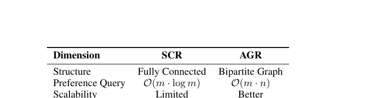
Dimension	SCR	AGR
Comparison structure	Fully connected tournament	Bipartite graph (responses vs. anchors)
Preference queries	$N_{\text{SCR}} = \frac{m(m-1)}{2}$	$N_{\text{AGR}} = m\cdot n$
Scalability (large $m$)	Limited (quadratic)	Better (linear in $m$, for fixed $n$)

Query-cost derivation. The exact query counts are $N_{\text{SCR}} = \binom{m}{2} = \frac{m(m-1)}{2}$ and $N_{\text{AGR}} = mn$. The difference:

$$N_{\text{SCR}} - N_{\text{AGR}} = m\left(\frac{m-1}{2} - n\right), \tag{28}$$

which is positive whenever $n < \frac{m-1}{2}$ — a typical regime in practice (the paper uses $n=8$ against sampling group sizes $m=8$ or $16$, so this condition is easily satisfied once $m>17$; even at $m=8$, $n=8 > \frac{7}{2}=3.5$ means AGR is actually more expensive per-pair at that particular small scale, but AGR wins overall efficiency once you factor in that anchors are precomputed once and reused across all prompts and all training steps, whereas SCR’s comparisons are prompt-specific and must be redone every step). Up to constant factors, the gap scales as $m(m-n)$ for $n<m$, which is the formal statement of “AGR scales better as the sampling budget $m$ grows.”

6. Experiments

6.1 Setup

Backbones. Reward models: LLaMA-3.2-3B-Instruct and LLaMA-3.1-8B-Instruct. Policy: LLaMA-3.1-8B-Instruct for the main table, with a cross-check on Qwen2.5-7B-Instruct (Table 2) to test backbone generality.

Data. Reward model training: HelpSteer3 (40.5K labeled examples with human rationales, used as CoT supervision for GRMs; DRMs get only the binary label, for a controlled comparison). RL training: SFT set of 6K examples, RL set of 7.5K examples, following the setup of Bhaskar et al. (2025).

RL algorithm. GRPO, learning rate $1\times10^{-6}$, batch size 128. Group size $m=8$, anchor set size $n=8$ in the main table. Two policy variants are trained: with explicit CoT (“w/ Thinking”) and without (“w/o Thinking”).

Evaluation. Open-ended chat: AlpacaEval2 (length-controlled win rate against a GPT-4-1106-preview reference, judged by GPT-4o, with a GPT-5 double-check evaluator), ArenaHardV2 (500 challenging real-world queries, same protocol), WildBench (1,024 prompts, point-wise 0-100 scoring). Reasoning/knowledge: MMLU-Redux, MATH-500 via evalscope.

Baselines. PRC (probability-based reward construction, Eq. 5) with and without a “removing thinking” variant that drops explicit CoT to reduce saturation; DRM; offline preference-optimization baselines DPO and SimPO trained on the same data.

6.2 Main results (Table 1)

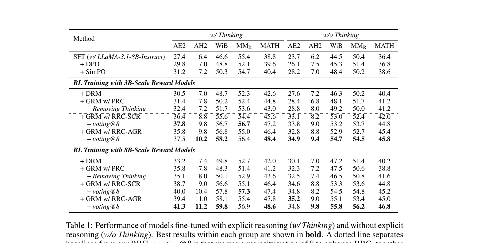
The headline numbers, 8B-scale reward models, w/ Thinking, AlpacaEval2:

Method	AE2
DRM	33.2
GRM w/ PRC	35.8
GRM w/ PRC + Removing Thinking	35.1
GRM w/ RRC-SCR	38.7
GRM w/ RRC-SCR + voting@8	40.0
GRM w/ RRC-AGR	39.4
GRM w/ RRC-AGR + voting@8	41.3

Three observations worth pulling out explicitly:

1. PRC barely beats DRM (35.8 vs. 33.2), consistent with the diagnostic experiment in §3 — probability-based construction wastes most of the GRM’s ranking advantage.
2. RRC roughly doubles the gain over DRM relative to PRC across essentially every benchmark and every scale (3B/8B) and every thinking mode.
3. Majority voting is a genuinely free lunch at this scale: voting@8 improves every RRC variant, with no observed downside in Table 1 (the cost trade-off shows up later, in Table 4).

The Qwen2.5-7B-Instruct cross-check (paper’s Table 2, not separately reproduced here as a figure) shows the same ordering and roughly the same magnitude of gains, which is the paper’s evidence that this isn’t a LLaMA-specific artifact.

6.3 Scaling behavior of RRC (§6.1, Figure 3)

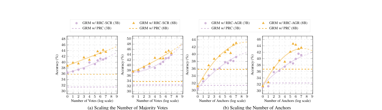
Two clean scaling-law-shaped curves: accuracy increases monotonically with the number of votes (panel a) and with the number of anchors (panel b), with visibly diminishing returns as either budget grows further — the textbook signature of a scaling law (the paper explicitly invokes Kaplan et al., 2020, for this framing). A specific and useful practical finding: a relatively small anchor count (8-16) already captures most of the achievable gain; pushing to 256 anchors actually causes a slight regression, which the paper attributes to a diversity problem — at very large anchor-sampling budgets it becomes harder to maintain sufficiently diverse anchor responses, so many anchors become redundant or low-information duplicates of each other rather than adding new comparison information.

6.4 Ablations (Figure 4 in the paper — the $\alpha$ and CARA ablations)

Sensitivity to the scaling factor $\alpha$. Sweeping $\alpha \in [0.05, 10.0]$, performance stays flat across $[0.05, 0.5]$ and degrades gradually beyond $\alpha=1.0$. The mechanistic explanation the paper gives (and it follows directly from the derivation in §4.1): GRPO’s group normalization (Eq. 4) is invariant to any positive affine rescaling of the reward, so moderate changes to $\alpha$ shouldn’t matter at all in principle — but once $\alpha$ gets large enough to interact with numerical clipping/other RL stabilizers (not explicitly detailed by the paper), noise gets amplified and training destabilizes. This is a case where the theory (§4.1’s Eq. 13, exact invariance) is a slight idealization, and the empirical ablation is honest about where that idealization breaks down.

CARA’s contribution. Removing Conflict-Aware Ranking Adjustment costs 0.6-1.9% on AlpacaEval2 and 1.3-1.5% on MMLU-Redux, consistently across both 3B and 8B backbones. Modest but consistent — cyclic inconsistencies in pairwise GRM judgments are real and resolving them via Kemeny-rule aggregation measurably helps, even if it isn’t the dominant lever (win-counting itself, i.e. RRC’s core idea, is the dominant lever; CARA is a refinement on top).

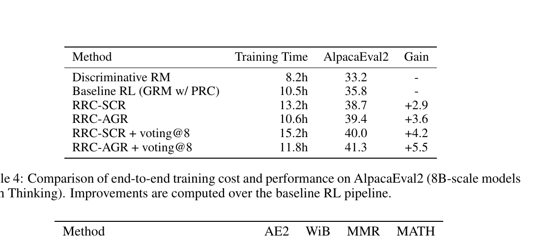
6.5 Efficiency: performance vs. training cost (Table 4)

Method	Training Time	AlpacaEval2	Gain
Discriminative RM	8.2h	33.2	–
Baseline RL (GRM w/ PRC)	10.5h	35.8	–
RRC-SCR	13.2h	38.7	+2.9
RRC-AGR	10.6h	39.4	+3.6
RRC-SCR + voting@8	15.2h	40.0	+4.2
RRC-AGR + voting@8	11.8h	41.3	+5.5

This table is arguably more important for a practitioner than Table 1: AGR gets a larger accuracy gain than SCR while adding almost zero training-time overhead relative to the PRC baseline (10.6h vs. 10.5h), because the anchor set is precomputed once (the paper reports ~1 hour on 16 GPUs) and reused across the entire training run, rather than requiring fresh pairwise comparisons every step the way SCR does. SCR’s higher accuracy-per-dollar-of-compute is real but comes at a real time cost (13.2h, a 26% increase over baseline). The paper’s own recommendation, reading between the lines of this table, is fairly clearly “use AGR unless you have a specific reason not to.”

6.6 Compute-matched comparison against a stronger PRC baseline (Table 5)

A natural objection to Table 1’s headline numbers: maybe RRC just wins because majority voting gives it more inference-time compute than plain PRC, and that alone explains the gain, independent of the ranking-vs-scoring idea. The paper controls for this directly by constructing a compute-matched PRC variant: instead of majority voting over the discrete A/B label, average the continuous preference probabilities from multiple CoT-enabled GRM queries (denoted “soft aggregation”), using the same number of GRM calls as RRC.

Method	AE2	WiB	MMR	MATH
GRM w/ PRC + Majority Voting	32.8	52.1	52.8	45.2
GRM w/ PRC + Soft Aggregation	30.1	51.4	48.2	44.8
GRM w/ RRC-SCR	36.4	55.6	54.4	45.6
GRM w/ RRC-AGR	35.8	56.8	55.0	46.4

Soft aggregation does not consistently beat plain majority-voted PRC (it’s actually worse on 3 of 4 benchmarks here), and both PRC variants remain clearly behind RRC despite using an equal number of GRM queries. This is good, clean evidence that the improvement is not just “more test-time compute” — it specifically comes from how the comparison signal is aggregated (structured, order-preserving win-counting vs. independent per-comparison probability averaging, which still inherits the saturation/confidence-confound problems of the underlying probability signal even after averaging).

6.7 A qualitative look: what does RRC actually change in the outputs? (Tables 7-8 in the paper)

The paper includes two full worked examples (a creative-writing rock-song task and a code-generation web-page task) where RRC-trained policies (SCR and AGR respectively) produce outputs that more faithfully track the prompt’s specific constraints (rhyme scheme + avoided-cliché-word list in the first case; exact hover-transition CSS behavior in the second) than the PRC baseline, which tends to drift toward generic, cliché-heavy or partially-correct outputs. These are illustrative single examples rather than systematic evidence, but they’re a useful sanity check that the aggregate benchmark numbers correspond to a real, qualitatively-visible behavior difference rather than a benchmark-gaming artifact.

7. Design Choices, Systematically: Why / Alternative / Boundary

To pull the scattered discussion above into one place, here are the paper’s five most consequential design decisions, each with the alternative it’s implicitly rejecting and the boundary condition under which the choice could fail:

Design choice	Why	Obvious alternative	Where it could fail
Win-counting rewards instead of probabilities	GRMs are trained to make comparative judgments, not calibrated scalar predictions (Eq. 2 vs. Eq. 1); win-counting is order-preserving and margin-aware by construction (§5.1)	Keep probability-based construction but try to de-saturate it (e.g., temperature scaling on the logits)	If the underlying pairwise judge is itself weak/noisy, win-counting amplifies rather than corrects that noise unless paired with voting/CARA
Reference-policy anchors (AGR)	Removes the moving-target/baseline-drift term from the policy gradient (Eq. 25-27), giving a stationary optimization objective	On-policy anchors, which auto-scale to current policy capability	Reference anchors become “too easy” late in training as the policy surpasses them, saturating $s_i \to n$; needs periodic refresh (not explored in the paper)
CARA / Kemeny-rule aggregation	Pairwise GRM judgments aren’t guaranteed transitive; Kemeny aggregation is the principled fix, with a clean proof that maximizing agreement = minimizing disagreement (Eq. 19-20)	Ignore cycles, use simple win-count sums directly (RRC’s own non-CARA fallback)	Exact Kemeny is NP-hard; the greedy heuristic (Davenport & Kalagnanam, 2004) is not guaranteed optimal, just empirically good
Majority voting over single queries	Individual GRM judgments are stochastic, especially under CoT; voting reduces judgment variance (§5.2)	Single deterministic (temperature-0) query per pair	Diminishing returns and real added inference cost (Table 4); doesn’t fix systematic bias, only variance
AGR over SCR as the default recommendation (implicit from Table 4)	Near-zero training-time overhead vs. PRC baseline, and comparable-or-better accuracy once anchors are precomputed	SCR, which extracts a somewhat larger raw accuracy gain (Table 5) at higher training cost	SCR wins when compute/time is not the binding constraint, or when the sampled group itself carries information anchors can’t (task-specific, in-context competitive dynamics)

8. Limitations

The paper’s own discussion of limitations is thin (it’s mostly implicit in the ablations rather than stated as a dedicated section), so I’ll consolidate what the data itself reveals:

• Anchor diversity degradation at scale (§6.3): performance saturates and can even regress with very large anchor counts (256), attributed to redundancy among sampled anchors, but this is only observed, not mechanistically diagnosed or mitigated in the paper.
• $\alpha$ sensitivity beyond the tested range (§6.4): the theory (§4.1) predicts exact scale-invariance under affine transforms, but the empirical ablation shows real degradation for $\alpha > 1$, which the paper attributes vaguely to “amplifying noise” without pinning down the specific mechanism (interaction with GRPO’s clipping? with optimizer numerics?).
• Reference-policy staleness is not addressed: as discussed in §5.7/Table above, AGR’s stability guarantee (Property 3) is bought at the cost of anchors that don’t adapt to the improving policy, and the paper never measures how large this gap grows over longer training runs than the ones reported (Table 1’s curves stop around 900 GRPO steps).
• Evaluated only on open-ended chat + a narrow reasoning slice: AlpacaEval2/ArenaHardV2/WildBench are all “helpfulness”-flavored open-ended benchmarks judged by other LLMs; MMLU-Redux and MATH-500 are the only reasoning-adjacent checks, and neither is a genuinely long-horizon agentic or verifiable-reward (RLVR) setting where reward hacking dynamics can look very different.
• Backbone and scale range is narrow: 3B/8B-scale GRMs, 7-8B policy models. Whether the probability-saturation problem (and hence RRC’s benefit) persists, worsens, or shrinks at frontier model scale (70B+ GRMs, or GRMs distilled from much stronger judges) is untested.

9. Critical Analysis

(a) Weaknesses and flaws specific to this paper.

1. Loose asymptotic notation for SCR’s query cost. The paper states $N_{\text{SCR}} = O(m\log m)$ in the main text (§4.2/§5.1) but the exact formula given a few lines later, and again in Appendix C.1, is $N_{\text{SCR}} = \binom{m}{2} = O(m^2)$ — genuinely quadratic, not $m\log m$. This isn’t a subtle distinction: it directly affects how a reader should reason about SCR’s scalability at large group sizes, and the paper’s own comparison table (Table 3) correctly labels SCR’s scalability “Limited” — consistent with $O(m^2)$, not $O(m\log m)$. This looks like a leftover from an earlier draft (perhaps SCR was once implemented via a tournament/sorting-network structure that really is $O(m\log m)$ comparisons, and the final all-pairs implementation superseded it without updating the complexity claim throughout).
2. The affine-faithfulness proof (§4.1) assumes something it doesn’t fully justify for SCR/AGR. The clean derivation in Appendix A shows that if $r$ is exactly affine in the oracle quality $q$ (Eq. 10), GRPO’s gradient is recovered exactly. But the paper never actually proves that SCR’s or AGR’s win-counting reward (Eq. 16/22) is affine in $q$ — it only shows margin awareness in the weaker proportionality sense (Eq. 17/23: reward differences correlate with quality differences, not that the map is exactly affine). These are related but not identical claims; win-counting is a bounded, integer-valued, saturating function of the pairwise-comparison count once a response beats (or loses to) everyone, which is itself a form of the very saturation problem the paper accuses PRC of — just at a coarser and less severe granularity (bounded by $m-1$ or $n$ rather than by $[0,1]$).
3. No error bars, no seed count reported anywhere in the main tables. Every number in Table 1 (and 2, 4, 5) is a single point estimate. Given that GRPO training is known to have meaningful run-to-run variance, and that some of the reported deltas (e.g. CARA’s 0.6% gain on one benchmark) are within a plausible noise band for a single seed, this materially weakens confidence in the smaller ablation deltas specifically (the headline RRC-vs-PRC gaps of 3-6 points are large enough to likely survive seed variance, but the finer-grained comparisons — SCR vs AGR, with vs without CARA, voting@4 vs voting@8 — are exactly the numbers a reader would want error bars for and doesn’t get them).
4. The judge-model dependency is not stress-tested. Both the RL reward signal (the GRM being trained/used) and the final evaluation (AlpacaEval2/ArenaHardV2’s GPT-4o/GPT-5 judges) are LLM-based judgments. The paper doesn’t check whether RRC’s gains are an artifact of correlated biases between the training-time GRM and the evaluation-time judge (e.g., both preferring longer, more structured, or more confidently-worded responses) — a well-known confound in LLM-judged RLHF evaluation generally, and one this paper is not unusually careful about relative to the field’s current best practices (e.g., no swap-judge or human-verification cross-check is reported).

(b) Limitations the authors understate or omit.

1. The paper frames GRM-vs-DRM entirely around ranking accuracy transferring (or not) into RL gains, but never squarely engages with the cost side of the comparison: a GRM query (generate + parse a judgment, optionally with CoT) is substantially more expensive per call than a DRM’s single forward pass to a scalar head. Table 4 reports wall-clock training time, which implicitly bakes this in, but the paper never states the per-query cost ratio explicitly, making it hard for a reader to reason about whether RRC’s gains would still be worth it at, say, 10x the GRM inference cost of the reported setup, or in a budget-constrained setting where a much cheaper DRM ensemble might be a better use of the same compute.
2. AGR’s anchor-quality dependency is real but under-explored: the paper shows reference-policy anchors are more stable than on-policy anchors (Property 3), but never demonstrates that they’re of high enough absolute quality to be a useful discrimination yardstick in the first place — if the reference policy is weak, AGR’s rewards could be uniformly high (everyone beats a bad reference) with little discriminative power, independent of the drift argument.
3. The paper’s related-work section frames itself as the first to move from “scalar reward from GRM” to “ranking-based reward from GRM,” but concedes in passing that Song et al. (2025) also investigated “reference-based reward construction for generative reward models” — the paper distinguishes itself by claiming Song et al. still derives scalar rewards from reference comparisons, but doesn’t go into enough technical detail about that prior work for a reader to independently verify how substantive the distinction is.

(c) Concrete, specific improvement suggestions.

1. Fix the SCR complexity notation throughout (§4.2, §5.1, Appendix C.1) to consistently state $O(m^2)$, and either implement or explicitly note as future work a genuinely $O(m\log m)$ tournament-sort-based variant of SCR (e.g., merge-sort-style pairwise comparisons with a comparator queried from the GRM), which would make the “SCR: Limited scalability” row in Table 3 an engineering choice rather than a hard mathematical ceiling.
2. Report multi-seed results with error bars/confidence intervals for at least the ablation tables (CARA on/off, voting@V sweep, $\alpha$ sweep), even if the main Table 1 headline comparisons remain single-seed due to compute constraints — this is the standard the RL-for-LLMs literature should be holding itself to given how well-documented GRPO’s run-to-run variance is.
3. Add a periodic anchor-refresh ablation for AGR: train with reference-policy anchors refreshed every $k$ GRPO steps (for a few values of $k$, including $k=\infty$ as the current no-refresh setting) and report whether this recovers additional gains in late training without reintroducing the moving-target instability of fully on-policy anchors — this would directly test the boundary condition flagged in §5.7/§8 above and turn a known theoretical limitation into an empirically characterized trade-off curve.
4. Report a judge-swap or held-out human-preference cross-check for at least a subset of the AlpacaEval2/ArenaHardV2 evaluation, using a judge model architecturally unrelated to both the training-time GRM and the primary evaluation judge, to rule out correlated-bias inflation of the reported gains.

10. Reproducibility Notes

• Code released: https://github.com/wangclnlp/RRC (linked in the abstract).
• Backbones fully specified: LLaMA-3.2-3B-Instruct / LLaMA-3.1-8B-Instruct for reward models; LLaMA-3.1-8B-Instruct and Qwen2.5-7B-Instruct for the policy.
• Data: HelpSteer3 (public, 40.5K examples) for reward model training; SFT (6K) / RL (7.5K) sets following Bhaskar et al. (2025) — these downstream sets are not independently re-specified in this paper, so full reproduction requires also obtaining that prior work’s exact data splits.
• Hyperparameters given: reward-model training LR $1\times10^{-5}$, batch size 256, 1 epoch; GRPO LR $1\times10^{-6}$, batch size 128; RRC scaling factor $\alpha = 0.1$; group size $m=8$ (with $m=16$ used only in the scaling-behavior study, Figure 3); anchor set size $n=8$ (main table), swept up to 256 in Figure 3.
• Not fully specified / would block exact reproduction: the exact number of GRPO training steps used for the main Table 1 numbers (Figure 1’s curves run to 900 steps, but Table 1 doesn’t state which checkpoint-selection step was used beyond “checkpoint saved every 100 steps, best selected on a 500-example validation set scored via AlpacaEval2 protocol with GPT-4o”); the precise CoT judging prompt template given to the GRM; random seeds (none reported, as noted in the Critical Analysis); the exact vLLM deployment configuration beyond “8 GPUs, 8 model instances” for reward-serving parallelism.
• Compute: reported training times (Table 4) are 8.2-15.2 hours per run on an unspecified but implied fixed hardware budget (not stated in GPU-count/GPU-type terms bewithin the main text; only the anchor-generation step is explicitly pinned to “16 GPUs, ~1 hour”).

11. Conclusion

RRC’s central claim is narrow but well-supported: the bottleneck preventing generative reward models from translating their strong pairwise-judging ability into strong RL training signals is not the GRM itself, but the specific mechanism (probability-based scalar extraction) used to bridge GRM judgments into the scalar-reward interface that GRPO-style RL expects. Replacing that bridge with structured, ranking-based aggregation — win-counting over exhaustive pairwise comparisons (SCR) or against a small stable anchor set (AGR), stabilized with majority voting and made globally consistent with Kemeny-rule conflict resolution (CARA) — recovers most of the gap, roughly tripling the RL-side gain over a discriminative baseline (from +1.3% to +5.5% on AlpacaEval2 with the best RRC configuration) without requiring any change to the GRM’s own training objective. The theoretical core (§4.1’s exact cancellation of affine reward transforms under GRPO’s group normalization) is genuinely illuminating and, as far as I can tell, correctly executed — it’s the kind of small, sharp derivation that clarifies why a class of engineering fixes should be expected to work, rather than just reporting that one particular fix happened to work. The gaps are mostly in rigor-of-evidence (single-seed tables, an imprecise complexity claim, thin exploration of anchor staleness) rather than in the core idea, which reads as a solid, useful contribution to the very active generative-reward-model literature.