ContextPilot: Teaching LLM Agents to Manage Their Own Context with Fine-Grained RL

Review date: 2026-08-31 Paper reviewed: ContextPilot: Teaching Agents for Proactive Context Management via Fine-grained RL Paper authors: Zhuoshi Pan, Qizhi Pei, Junru Lu, Honglin Lin, H. Vicky Zhao, Di Yin, Xing Sun (Tsinghua University, Tencent Youtu Lab, Shanghai AI Lab) arXiv: 2608.28476 Venue/Status: arXiv preprint, submitted 28 Aug 2026

1. What Problem Is This Paper Actually Solving?

Picture an LLM agent doing “deep research”: it gets a question, it searches the web, it reads a document, it searches again, it reads another document, and so on for dozens of turns before it can answer. Every tool call and every tool response gets appended to the conversation — the agent’s “context” — because the standard ReAct-style loop treats the full interaction history as the ground truth of what happened so far. The problem is obvious once you say it out loud: that context only grows. After 20-30 turns on a genuinely hard question, you can easily be carrying tens of thousands of tokens of half-relevant search results, and every subsequent LLM call has to re-read all of it, burning latency, money, and — worse — attention budget that could have gone toward the actually-relevant facts.

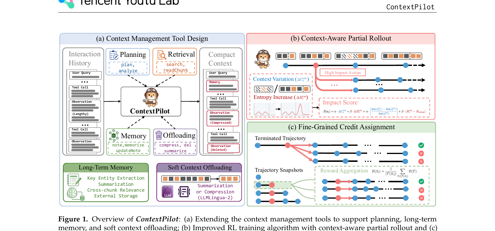
This paper is about proactive context management: giving the agent itself a set of tools to edit its own working context (delete stale tool outputs, summarize a block of history, write a note to itself, etc.) rather than relying on some external, rule-based system that truncates or summarizes on a fixed schedule. This idea isn’t new — the paper builds directly on a line of prior work (MemGPT, StateLM, Sculptor, MemAct, AgentFold) that already gives agents some context-editing tools. But the authors identify three concrete gaps in that line of work, and building a fix for each gap is the entire content of the paper:

1. The toolset is too narrow. Existing systems mostly offer search, delete, and summarize. There’s no explicit planning tool, no persistent long-term memory structure, and no graduated (“soft”) compression options — it’s binary keep-or-throw-away.
2. RL training treats all context-editing actions as equally important, when empirically they are not — some edits (like deleting a big chunk of history) can completely derail a trajectory, while others barely matter.
3. Credit assignment is too coarse. When an agent’s trajectory finally succeeds or fails, existing methods assign that single win/loss reward to every intermediate context-editing decision along the way, even though those decisions had very different local importance and even though many terminal outcomes are more a matter of luck in retrieval than of good context hygiene.

ContextPilot’s contribution is threefold, matching these three gaps one-to-one: (1) a richer toolset (planning + long-term memory + soft offloading tools bolted onto the existing search/delete/summarize toolkit), (2) a rollout scheme that spends extra sampling budget specifically on the context-editing decisions that seem to matter most (“context-aware partial rollout”), and (3) a lower-variance way to estimate how good an intermediate context-editing decision was, using all the trajectories that pass through it rather than just the one trajectory that happened to be sampled (“fine-grained credit assignment”). Experiments on four long-context QA benchmarks and four deep-search benchmarks show consistent gains of 2-5 points over the strongest prior context-management baseline (StateLM) and over vanilla GRPO training, while using a smaller context window (32K) than an untouched 128K-context backbone.

2. Prerequisites: What You Need to Understand First

2.1 The ReAct loop and why context grows monotonically

Most modern tool-using LLM agents follow the ReAct pattern (Yao et al., 2023): at each step $i$, given the current context $c_i$ (everything that has happened so far — the user’s question, prior thoughts, prior tool calls, prior tool outputs), the policy model $\pi_\theta$ samples a thought and a tool call:

$$(t_i, a_i) \sim \pi_\theta(\cdot \mid c_i). \tag{1}$$

The environment then executes the tool call and returns an observation $o_i \sim \mathcal{E}(\cdot \mid a_i)$, and everything gets appended to form the next context:

$$c_{i+1} = c_i \oplus (t_i, a_i, o_i). \tag{2}$$

The $\oplus$ here is literal concatenation. There is no forgetting mechanism built into the loop itself — this is why context grows monotonically. If you run this loop for 30 turns on a task that needs several rounds of web search over long documents, you can accumulate hundreds of thousands of tokens, most of which (failed searches, partially relevant chunks, dead-end reasoning) will never be useful again but still costs money and attention to re-process at every subsequent step.

2.2 Reinforcement learning for LLM agents: GRPO in one paragraph

To train an agent policy $\pi_\theta$ with RL, a common recent recipe is GRPO (Group Relative Policy Optimization), used because it avoids training a separate value/critic network. For a given input (here, a query $q$), you sample a group of $G$ complete trajectories/responses, score each with a reward function, and compute each sample’s advantage as its reward normalized against the group’s own mean and standard deviation:

$$\hat{A}^{(j)} = \frac{R^{(j)} - \text{mean}(\{R^{(1)}, \dots, R^{(G)}\})}{\text{std}(\{R^{(1)}, \dots, R^{(G)}\})}. \tag{3}$$

This is a group-relative baseline instead of a learned value function — cheap and stable, provided the group of samples is reasonably diverse and reasonably sized. ContextPilot’s entire training-side contribution can be summarized as: what if the “samples” in the GRPO group weren’t whole trajectories, but individual snapshots of a trajectory taken between context-editing operations? We’ll unpack exactly what that means below.

2.3 What “context editing” means precisely, and why it breaks naive RL

Let $\mathcal{A}$ be the full action space available to the agent (all tools), and let $\mathcal{A}_{\text{cm}} \subseteq \mathcal{A}$ be the subset of context management actions. Within that, define $\mathcal{A}_{\text{ce}} \subseteq \mathcal{A}_{\text{cm}}$ as context editing actions — the subset that actually rewrites the interaction history (as opposed to, say, a plan call that just adds a new thought without deleting anything). When the model invokes a context-editing action $a_i^{\text{cm}} \in \mathcal{A}_{\text{cm}}$, the context transitions via a transition function $\mathcal{F}$ rather than simple append:

$$c_{i+1} = \mathcal{F}(c_i, a_i^{\text{cm}}) \oplus (t_i, a_i, o_i). \tag{4}$$

For example, if $a_i^{\text{cm}}$ is deleteContext(msg_id=7), then $\mathcal{F}$ replaces message 7 with a placeholder, and everything downstream of that point sees a shorter history than everything upstream. This is the crux of why naive full-trajectory RL training breaks down here: if you train on full trajectories with standard next-token loss, the model would be asked to predict tokens conditioned on a context that includes message 7 in full (before the delete) and tokens conditioned on a context where message 7 has already been replaced by a placeholder (after the delete) — inconsistent training signal for the same underlying trajectory. Prior work (StateLM, Sculptor) already solved the training-signal half of this problem with trajectory snapshots: cut the trajectory into pieces at every context-editing action, and treat each piece as an independent training example, with token-level loss masking so you don’t re-optimize over content that already appeared in an earlier snapshot. If a trajectory contains $K$ tool calls total, of which $M$ are context-editing operations, it gets segmented into $M+1$ snapshots $\mathcal{S} = \{S_1, \dots, S_{M+1}\}$.

What prior work had not solved is the reward-signal half of the same problem — and that’s ContextPilot’s real contribution. Even with clean snapshot-level training data, you still need to decide what reward each snapshot gets. Naively, you’d give every snapshot in a trajectory the same final win/loss reward $R(T)$. ContextPilot argues (with direct empirical evidence, Figure 2 below) that this is a bad idea, because different context-editing decisions have wildly different influence on the final outcome, and because a single trajectory’s terminal reward is a noisy, high-variance signal for judging any one intermediate decision.

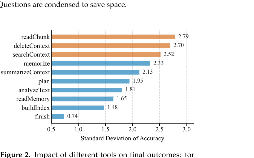
Figure 2 is the paper’s motivating evidence for why not all context-management actions deserve equal RL exploration budget: if you branch off ten separate continuations from the same point right after a readChunk or deleteContext call, the resulting success rates vary a lot (std ≈ 2.5-2.8), whereas branching after finish (which ends the trajectory) trivially has near-zero variance (std ≈ 0.74) because there’s nothing left to explore. The tools in the orange bars — readChunk, deleteContext, searchContext — are the ones where “what you do here” genuinely swings the final answer; the blue bars are comparatively low-stakes. This single figure is the empirical seed for the entire “context-aware partial rollout” mechanism described in Section 4.

Complementing this, Figure 3 shows the flip side of the same coin: correctness and “good context management” are not the same axis, and rewarding one as a proxy for the other is unreliable.

On the left, the agent gets the right answer (Robert D. McBain) despite a messy tool chain that repeats search 3 times and reads chunks over and over — brute-force retrieval that happens to land on the answer. On the right, the agent uses a textbook-clean context-management strategy (note → delete → search → updateNote → delete → readNote → finish) but still lands on the wrong answer (Ty Longley instead of Frank Leepa), presumably because the retrieved evidence itself was misleading. If you train by assigning the trajectory’s final reward to every intermediate context-editing step, the left trajectory teaches the model “messy management is fine” and the right trajectory teaches it “clean management doesn’t help” — both false lessons induced purely by trajectory-level credit assignment being too coarse. This is exactly the failure mode that motivates fine-grained, snapshot-level credit assignment.

3. Method: Toolset, SFT Data, and the RL Recipe

3.1 The extended context management toolset

Table 1 in the paper (reproduced below) lists the full toolset ContextPilot equips the agent with. Rows in bold/highlighted categories are the paper’s new additions on top of the base StateLM toolset (search, delete, summarize).

Category	Tool Name	Function
Perception & Planning	analyzeText	Calculate context length
Perception & Planning	checkBudget	Check remaining token budget
Perception & Planning	plan	Propose a concise plan
Information Retrieval	buildIndex	Build a searchable index
Information Retrieval	searchContext	Search for relevant content
Information Retrieval	readChunk	Load a specific context chunk
Information Retrieval	readMultiChunks	Batch-load multiple chunks
Memory Management	note / updateNote / readNote	Short-term scratchpad notes
Memory Management	memorize	Extract entities/timestamps/event episodes into structured long-term memory, with edges linking related items
Memory Management	updateMemory / readMemory	Update/retrieve a structured memory item
Context Offloading	deleteContext	Replace a message with a placeholder
Context Offloading	summarizeContext	Replace a message with a summary
Context Offloading	compressContext	Compress a message via a lightweight external model (LLMLingua-2)
Context Offloading	foldHistory	Discard all history, keep only a searchable index recoverable via keyword search

Why bother adding plan at all, when the model could presumably “just think” before acting? The design choice here is to make planning an explicit, callable tool rather than leaving it implicit in the chain-of-thought, because that gives the harness (and later, the RL reward function) a hook to enforce and reward planning behavior specifically — an implicit plan buried inside free-form reasoning text is invisible to a rule-based reward or a token-position-based credit assignment scheme; an explicit plan call is not. The obvious alternative (no separate plan tool, just prompt the model to “think step by step”) was in fact the status quo in ReAct-style agents, and the ablation in Table 4 (Section 5) shows a real, measurable accuracy gain from making it explicit (NovelQA 88.90 → 89.76, BrowseComp+ 63.49 → 65.66) — a modest but consistent gain, suggesting the value of making planning a first-class, budgeted action rather than free-floating text.

The memorize/readMemory pair is the most structurally different addition. Rather than a flat note (single blob of scratch text), memory items are extracted with typed structure (entities, timestamps, event episodes) and connected via edges to related items, so a later readMemory call retrieves not just one fact but its immediate neighborhood in a small knowledge graph. The design tradeoff here: a flat note is trivial to construct and read but doesn’t compose (“if I wrote two related facts as two separate notes, retrieving one doesn’t surface the other”); a graph-structured memory needs an extraction/linking step (more work per write, more chance of extraction errors) but composes (“retrieving one memory pulls in what’s causally/referentially close to it”). Table 4’s ablation shows this is the single largest incremental improvement of the four toolset additions — BrowseComp+ jumps from 71.20 (with only planning + soft offloading) to 80.96 once long-term memory is added, a +9.76 point jump, the biggest single increment in the whole table. This makes sense specifically for BrowseComp+, which is built from very long, information-dense documents (552K tokens on average) where a flat note-taking approach would produce an unmanageably long, unstructured scratchpad; graph-structured memory is what lets the agent retrieve just the relevant sub-cluster of facts instead of re-scanning everything.

The context-offloading side introduces three levels of “softness” beyond a hard delete: summarizeContext (lossy but human-readable compression), compressContext (uses LLMLingua-2, a dedicated small compression model, to shrink text while preserving more of the raw signal than a summary would, at the cost of readability), and foldHistory (the most aggressive — throw away the actual text entirely, keep only a searchable index, and force the agent to re-search by keyword if it later needs something it folded away). The obvious alternative to offering three separate mechanisms would be to pick one (say, just summarization) and rely on the model learning when to be more or less aggressive with it. The paper’s design bet is that giving the model discrete choices about compression aggressiveness, rather than one compression operator applied uniformly, lets RL training learn a policy over which compression mode fits which situation — e.g., fold a stale search-result branch entirely (since it’s unlikely to be revisited) but only summarize (not fold) a chunk that’s still actively load-bearing for the current sub-goal. The boundary case where this design can fail: if the model mis-judges which branch is “stale” and folds something it needs again, foldHistory’s aggressive discard-of-raw-text means recovery is limited to keyword search over an index — strictly lossier than summarizeContext’s recoverable summary. The paper does not report a separate ablation isolating foldHistory specifically from summarizeContext/compressContext, so we cannot tell from the numbers alone how often this failure mode actually bites in practice — a gap we return to in the critical analysis (Section 7).

3.2 Building the SFT data (bootstrapping via a teacher + harness)

Before any RL, ContextPilot needs supervised fine-tuning (SFT) data that demonstrates competent use of this new, larger toolset — an RL policy that has never seen memorize used correctly even once has essentially no chance of discovering it through exploration alone in a reasonably-sized training run. The SFT data pipeline (Algorithm 1 below, reconstructed from Appendix C) uses a strong teacher model (Qwen3.5-397B-A17B in “thinking” mode) generating trajectories under a harness — a rule-based scaffold that dynamically restricts which tools are visible/callable at each step based on preconditions.

Algorithm 1 — SFT Trajectory Synthesis with Harness Scaffolding

Input: question set Q, teacher model π_teacher, harness H, max_retries = 2
Output: filtered trajectory snapshot set D_SFT

1  D_raw ← ∅
2  for each question q in Q:
3      trajectory T ← ∅ ; context c ← [q]
4      while not finished(T) and steps(T) < max_steps:
5          available_tools ← H.get_available_tools(c)      # e.g. hide readChunk
                                                              # until searchContext used
6          (thought, action) ← π_teacher(c ; available_tools)
7          if H.is_invalid(action, c):                       # e.g. deleteContext on
                                                              # an already-deleted id
8              hint ← H.generate_correction_hint(action, c)
9              c ← c ⊕ hint                                  # ask teacher to retry
10             retry_count += 1
11             if retry_count > max_retries: discard trajectory; break
12             continue                                      # loop back to step 6
13         observation ← Environment.execute(action)
14         c ← F(c, action) ⊕ (thought, action, observation)  # Eq. 2 / Eq. 4
15         T ← T ⊕ (thought, action, observation)
16     D_raw ← D_raw ∪ {T}
17
18  # Stage 1: outcome-based filtering (exact match against gold answer)
19  D_stage1 ← { T ∈ D_raw : is_correct(T) OR ∃ retry T' with is_correct(T') }
20
21  # Stage 2: process-based filtering with an auxiliary judge model
22  D_stage2 ← { T ∈ D_stage1 : GPT-OSS-120B_judge(T) says
                 "context management is proper" }
23
24  # Stage 3: peak-context filtering
25  D_stage3 ← { T ∈ D_stage2 : max_context_length(T) ≤ 32K tokens }
26
27  # Segment each retained trajectory into snapshots at context-editing actions
28  D_SFT ← ∅
29  for T in D_stage3:
30      snapshots ← segment_at_context_editing_actions(T)     # Eq. 4's a_ce actions
31      D_SFT ← D_SFT ∪ snapshots
32
33  return D_SFT

A few numeric details worth internalizing, straight from Appendix C/Table 6: starting from 3,196 questions, outcome-based filtering (line 19) keeps 3,114 trajectories, and the process + peak-context filters (lines 22, 25) remove another 46, leaving 3,068 qualified trajectories, which segment into 51,469 SFT snapshots — roughly 17 snapshots per trajectory on average, giving a sense of how often context-editing actions actually fire in a realistic long-horizon trajectory. Two design choices in this pipeline deserve explicit “why/alternative/boundary” scrutiny:

• Why a harness with dynamic tool visibility, rather than exposing the full toolset at every step? The alternative — always show all 14 tools — would let the teacher call readChunk before ever calling searchContext (there’d be nothing to read), or call readMemory before any memory exists. Rather than relying on the teacher model to self-regulate (which a merely-strong-but-imperfect teacher won’t reliably do, especially under sampling temperature 0.6), the harness enforces preconditions structurally. The boundary case: this scaffolding is stripped from the final SFT trajectories (line 9’s hints never appear in $D_{\text{SFT}}$), so the policy being trained never sees the corrective hints — it only sees clean, successful action sequences. This is a deliberate choice to avoid teaching the student to need correction, but it does mean the student never learns an explicit self-correction skill from SFT; any recovery-from-mistake behavior has to be learned later, during RL, from scratch.
• Why filter with a separate judge model (GPT-OSS-120B) rather than trusting outcome-correctness alone? Section 3.2/Figure 3 already showed that outcome correctness and context-management quality are not the same thing (a correct answer can come from messy management, per Figure 3’s left case). If the SFT set were filtered by outcome alone, it would happily include the left-hand case in Figure 3 as a positive example, teaching the model to imitate messy-but-lucky retrieval. The judge model is an attempt to filter on the process axis independently of the outcome axis. The obvious risk: the judge itself is an LLM with its own blind spots and biases, and the paper reports no inter-annotator agreement or human-audit numbers for how reliable this judge actually is at telling good from bad context management — a real reproducibility gap we flag again in Section 7.

3.3 RL training: context-aware partial rollout

This is the paper’s first genuinely novel training-side mechanism. Standard GRPO samples $G$ complete trajectories per query and computes group-relative advantages. ContextPilot instead wants extra branching specifically at the context-editing decisions that seem most consequential (recall Figure 2’s variance argument). To decide where to branch, it defines two per-action signals.

Context variation measures how much the context length changed relative to its pre-edit length:

$$\Delta C_t^{\text{cm}} = \frac{\text{len}(c_{t+1}^{\text{cm}}) - \text{len}(c_t^{\text{cm}})}{\text{len}(c_t^{\text{cm}})}. \tag{5}$$

Here $c_t^{\text{cm}}$ denotes the context right before the context-management action at step $t$, and $c_{t+1}^{\text{cm}}$ the context right after. This is negative for a deleteContext/foldHistory (context shrinks) and near-zero (or slightly positive, if a summary is longer than expected) for milder edits — it’s a cheap, direct proxy for “how drastic was this edit.”

Entropy variation measures how much the model’s own generation uncertainty shifted relative to the start of the trajectory (not the immediately preceding step):

$$\Delta H_t^{\text{cm}} = H_t^{\text{cm}} - H_{\text{initial}}, \tag{6}$$

where the entropy of a window of $k$ generated tokens after an observation at step $t$ is the standard token-level Shannon entropy averaged over the window:

$$H_t^{\text{cm}} = \frac{1}{k}\sum_{i=0}^{k-1}\left(-\sum_{j=1}^{V} p_{t+i,j}\log p_{t+i,j}\right), \tag{7}$$

with $V$ the vocabulary size and $p_{t+i,j}$ the softmax probability of token $j$ at position $t+i$. Why compare against the initial entropy $H_{\text{initial}}$ rather than the entropy of the immediately preceding step $H_{t-1}^{\text{cm}}$? The paper’s stated reasoning: partial rollout is meant to catch context edits that induce large uncertainty shifts relative to the model’s baseline confidence at the start of the task, not small step-to-step wobbles that are likely just noise. The design alternative (comparing consecutive steps) would be noisier and more sensitive to any single unlucky sampling step; anchoring to the trajectory’s start gives a more stable reference point, at the cost of not detecting a genuine local anomaly if the whole trajectory has been drifting into high-entropy territory gradually (in which case $\Delta H_t^{\text{cm}}$ would look large even for an unremarkable step, simply because everything after the first few steps is already elevated).

Combining both signals gives a scalar sensitivity score:

$$S(a_t^{\text{cm}}) = \alpha \cdot \Delta C_t^{\text{cm}} + \beta \cdot \Delta H_t^{\text{cm}}, \tag{8}$$

with $\alpha = \beta = 1$ in the paper’s experiments (no hyperparameter search reported over this weighting — flagged in Section 7). The rollout procedure itself:

Algorithm 2 — Context-Aware Partial Rollout

Input: query q, policy π_θ, snapshot budget N, per-query trajectory rollouts G_0 = 8
Output: snapshot pool P for GRPO training on this query

1  P ← ∅
2  # Phase 1: full trajectory-level rollouts
3  for i = 1 to G_0:
4      T_i ← rollout_full_trajectory(π_θ, q)      # Eq. 1-2/4
5      S_i ← segment_at_context_editing_actions(T_i)   # up to 8 snapshots per trajectory
6      P ← P ∪ S_i
7  M ← |P|                                        # up to G_0 * 8 = 64 snapshots so far
8
9  # Phase 2: allocate remaining budget to partial rollout at high-sensitivity points
10 if M < N:
11     candidates ← all context-editing actions observed across the G_0 trajectories
12     for a_t^cm in candidates:
13         compute S(a_t^cm) via Eq. 8
14     ranked ← sort candidates by S(a_t^cm) descending
15     branch_points ← top (N - M) actions from ranked
16     for each selected branch point b (with parent context c_b):
17         T_branch ← rollout_continuation(π_θ, starting_from=c_b)
18         S_branch ← segment_at_context_editing_actions(T_branch)
19         P ← P ∪ S_branch
20
21 return P    # |P| = N snapshots total, feeding into GRPO (Eq. 3/10)

With the paper’s concrete numbers: $N=128$ snapshots per query, $G_0=8$ initial full rollouts, each capped at 8 snapshots (so up to $M=64$ from Phase 1), leaving up to 64 more snapshots’ worth of budget for Phase 2’s targeted partial rollout. The design rationale for spending half the budget on targeted branching rather than, say, just sampling 16 full trajectories instead of 8 (which would also give roughly 128 snapshots via Phase 1 alone): full trajectories spend their entire sampling cost exploring every decision point uniformly, including the low-variance ones (Figure 2’s finish, buildIndex) that don’t need more exploration. Partial rollout concentrates the marginal sampling budget specifically where Figure 2 says the payoff is highest. The ablation in Table 5 (Section 5.4) shows this matters: adding entropy-based partial rollout alone is actually unstable (BrowseComp+ drops by 1.32 points relative to plain GRPO), while adding the context-variation signal on top stabilizes and improves it (+1.44 over GRPO) — a concrete, reported instance of a design choice that doesn’t work in isolation, which is refreshingly rare for a paper to show.

3.4 Fine-grained credit assignment

Once you have this pool of trajectory snapshots (some from full rollouts, some from partial rollouts branching off high-sensitivity points), how do you reward an intermediate snapshot $S_i$ that isn’t itself a complete, terminated trajectory? The paper’s answer: average the outcome rewards of every terminal trajectory that has $S_i$ as a prefix.

For a terminal snapshot $S_M = T$ (a complete trajectory), the reward decomposes into three additive terms:

$$R(S_M) = R_{\text{out}} + R_{\text{fmt}} + R_{\text{pen}}. \tag{9}$$

$R_{\text{out}}$ compares the predicted answer against ground truth (correctness); $R_{\text{fmt}}$ checks whether the final output is even parseable; $R_{\text{pen}}$ is a penalty for invalid tool invocations — e.g., calling readMemory before any memory item has been written, or violating a context-length budget. This penalty term is worth pausing on: without it, a policy that happens to stumble on the correct answer despite egregious tool misuse (imagine calling readMemory on a nonexistent key ten times before finally guessing right) would receive full positive reward, actively reinforcing the misuse. $R_{\text{pen}}$ exists specifically to prevent Figure 3’s “correct answer, bad process” pathology from leaking into what the terminal reward itself represents, even before you get to the credit-assignment question of how that reward propagates to intermediate snapshots.

For an intermediate snapshot $S_i$, its reward is the average terminal reward over the set $\mathcal{T}(S_i)$ of all sampled terminal trajectories that have $S_i$ as a prefix:

$$R(S_i) = \frac{1}{|\mathcal{T}(S_i)|} \sum_{T \in \mathcal{T}(S_i)} R(T). \tag{10}$$

This is the mathematical core of “fine-grained credit assignment,” and Appendix A gives a clean formal justification worth walking through in full, because it’s a genuinely satisfying piece of variance-reduction reasoning. Define the target credit for a snapshot $S$ as the true expected terminal reward conditional on $S$ having occurred:

$$Q(S) \triangleq \mathbb{E}[R(T) \mid S \preceq T], \tag{11}$$

where $S \preceq T$ means $S$ is a prefix of $T$. This $Q(S)$ is the ideal quantity you’d want to reward $S$ with — but it’s an expectation you can never observe exactly, only estimate from samples. Trajectory-level credit assignment (the old way) estimates it using just the one sampled continuation that actually happened:

$$\hat{Q}_{\text{traj}}(S) \triangleq R(T_1). \tag{12}$$

ContextPilot’s estimator averages over all $n_S = |\mathcal{T}(S)|$ sampled continuations:

$$\hat{Q}_{\text{ours}}(S) \triangleq \frac{1}{n_S}\sum_{k=1}^{n_S} R(T_k). \tag{13}$$

Both estimators are unbiased — this is a one-line consequence of linearity of expectation, since every $T_k$ is drawn from the same continuation distribution $p(\cdot \mid S)$:

$$\mathbb{E}[\hat{Q}_{\text{traj}}(S) \mid S] = \mathbb{E}[R(T_1)\mid S] = Q(S), \qquad \mathbb{E}[\hat{Q}_{\text{ours}}(S)\mid S] = \frac{1}{n_S}\sum_{k=1}^{n_S}\mathbb{E}[R(T_k)\mid S] = Q(S). \tag{14}$$

Where they differ is variance. Let $\sigma^2(S) \triangleq \text{Var}[R(T)\mid S \preceq T]$ be the true conditional variance of the terminal reward given $S$. The trajectory-level estimator, using a single sample, has variance exactly $\sigma^2(S)$:

$$\text{Var}[\hat{Q}_{\text{traj}}(S)\mid S] = \sigma^2(S). \tag{15}$$

ContextPilot’s estimator, being an average of $n_S$ conditionally-independent samples, has the classic sample-mean variance reduction:

$$\text{Var}[\hat{Q}_{\text{ours}}(S)\mid S] = \text{Var}\left[\frac{1}{n_S}\sum_{k=1}^{n_S}R(T_k) \,\middle|\, S\right] = \frac{1}{n_S^2}\sum_{k=1}^{n_S}\text{Var}[R(T_k)\mid S] = \frac{\sigma^2(S)}{n_S}. \tag{16}$$

Since both estimators are unbiased, their mean-squared error equals their variance, so whenever $n_S > 1$ and $\sigma^2(S) > 0$, the new estimator strictly dominates the old one in mean-squared error — a factor of $n_S$ reduction. This is exactly the textbook “sample-mean has lower variance than a single sample” result, applied here at the level of trajectory snapshots rather than i.i.d. data points, and it’s precisely why the earlier context-aware partial rollout mechanism matters practically: partial rollout is what inflates $n_S$ for the specific snapshots that most need a stable estimate (the high-sensitivity ones from Figure 2), so the variance reduction of Eq. 16 is concentrated exactly where the original problem (Figure 2/3) was worst.

After computing snapshot-level rewards via Eq. 10, all snapshots generated for the same query $q$ are grouped as $G = \{S_t^{(j)} \mid \forall j, t\}$, and the GRPO advantage (Eq. 3, restated at the snapshot level) is computed from this group’s own mean and standard deviation — so the group-relative baseline that used to operate over whole trajectories now operates over snapshots, giving every intermediate context-editing decision its own properly-scaled advantage signal rather than inheriting one trajectory’s lump-sum outcome.

4. Experiments and Results

4.1 Setup

Two task families are evaluated. Long-context QA: SFT on NovelQA (PublicDomain split) + NarrativeQA (training split), RL on LongBench-v2 (488 questions), evaluated on NovelQA-Copyright, ∞Bench (En.MC split), LongMemEval-S, and BrowseComp+ (built on a fixed, non-internet corpus, included here because it’s fundamentally a long-context retrieval task despite its search-flavored name). Base models: Qwen3-8B, Qwen3-14B, Gemma4-E4B-it. Deep search: RL directly on 1,000 sampled OpenSeeker questions (no SFT needed, since the base models WebSailor-7B and WebExplorer-8B already have search capability), evaluated on GAIA (text-only, 103 examples), BrowseComp, BrowseComp-ZH, xBench-DeepSearch.

Baselines for long-context QA: ReadAgent (training-free), MemAgent (RL-trained memory agent — labeled “RL-MemoryAgent” in the results table), StateLM (the direct predecessor proactive-context-management system), and a “w/ tools” ablation that gives the same extended toolset to an un-finetuned model (prompt-only). Baselines for deep search: plain ReAct, ReAct with fixed-threshold truncation, ReSum (inference-time summarization), SUPO (jointly RL-trains summarization + agentic ability), and OpenSeeker (same RL training data/setup as ContextPilot but without any context management tools).

4.2 Main results

The headline long-context QA numbers (Table 2 in the paper) show ContextPilot-8B-RL beating StateLM-8B-RL by an average of 3.55 points across the four benchmarks (69.40 vs. 65.85), and ContextPilot-14B-RL beating StateLM-14B-RL by 2.09 points (72.20 vs. 70.11) — while both use only a 32K context window. Perhaps the most striking single comparison: Qwen3.5-397B-A17B without any tools at all, using its native 256K context, scores 80.55 average, while the same model with the ContextPilot toolset (32K window) scores 87.16 — a 6.6 point improvement from shrinking the effective context and adding editing tools, not from adding capacity. This directly supports the paper’s framing: raw context capacity is not the bottleneck here, context hygiene is.

The deep-search results (Table 3) tell a similar story at a smaller scale. On WebSailor-7B, ContextPilot averages 38.32 across the four deep-search benchmarks vs. SUPO’s 36.31 and OpenSeeker’s 35.78 — modest but consistent gains, and the gap is largest specifically on BrowseComp (21.17 vs. SUPO’s 18.50, a 2.67-point gap) which is the hardest, most retrieval-intensive of the four.

4.3 Token efficiency: the practical payoff

Figure 4, reproduced below, is arguably the paper’s most intuitive result, because it visualizes the exact problem from Section 1 and the exact fix, side by side, without needing any benchmark-score table to interpret.

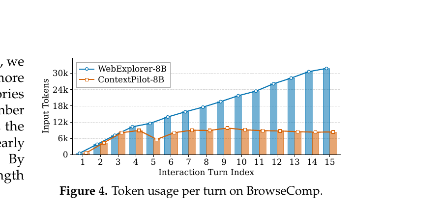
This is the direct visual confirmation of the paper’s central hypothesis: without context management, a genuinely long-horizon trajectory’s per-turn input cost keeps climbing (linearly here, and recall from Section 2.2 that attention cost scales quadratically in sequence length, so the compute cost of this growth is actually worse than the token count alone suggests). ContextPilot’s editing tools flatten this curve after roughly the fourth or fifth turn, meaning a trajectory that runs to turn 15 pays for a context window roughly 3x smaller than the uncontrolled baseline at that point — a very concrete, unit-economics-relevant result for anyone actually running these agents in production at scale (fewer tokens per LLM call directly means lower latency and lower per-query cost).

4.4 Ablations: which pieces actually matter

Table 4 (reproduced as a figure below) isolates the toolset contribution by cumulatively adding planning, then soft offloading, then long-term memory to a fixed backbone (Qwen3.5-397B-A17B), with no RL training involved (pure prompt-based tool availability):

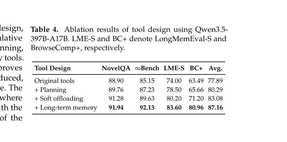
The pattern across all four benchmarks is monotone improvement as tools are added, with the biggest single jump coming from long-term memory (discussed already in Section 3.1) and the effect being most pronounced on BrowseComp+ specifically, consistent with that benchmark’s very long input documents (552K tokens on average) being exactly the regime where flat notes and simple deletion run out of steam.

On the RL-training side (Table 5, described in prose since it wasn’t separately cropped as a figure — see Section 3.3’s summary), the ablation shows: plain GRPO on top of SFT gives modest, somewhat inconsistent gains (+0.97 NovelQA, +1.75 ∞Bench, but -0.60 on LongMemEval-S); adding entropy-only partial rollout is actively unstable, hurting BrowseComp+ by 1.32 points; adding context-variation on top of entropy stabilizes things (+1.44 net on BrowseComp+ relative to plain GRPO); and adding fine-grained credit assignment on top of everything else delivers the largest and most consistent gains across all four benchmarks (+0.83, +1.31, +2.87, +3.10 respectively vs. plain SFT). The takeaway that the paper doesn’t state as bluntly as it could: the credit-assignment fix (Section 3.4) mattered more than the exploration fix (Section 3.3) in the reported ablation — the rollout mechanism alone was actually net-negative on one benchmark, and it’s the variance-reduced reward estimator that turns the combination into a consistent win.

To make the two-phase RL data pipeline (Algorithm 2, Section 3.3) concrete end-to-end, here is the flow from raw rollouts to a GRPO-ready snapshot pool:

flowchart TB
    A["Query q"] --> B["Phase 1: sample G0=8\nfull trajectory rollouts"]
    B --> C["Segment each trajectory\nat context-editing actions\n(up to 8 snapshots each)"]
    C --> D["Snapshot pool so far:\nM snapshots (M <= 64)"]
    D --> E{"M < N=128?"}
    E -- yes --> F["Compute sensitivity score\nS(a) = alpha*deltaC + beta*deltaH\nfor every context-editing action"]
    F --> G["Rank actions by S(a) desc,\npick top (N-M) as branch points"]
    G --> H["Phase 2: partial rollout\nfrom each branch point"]
    H --> I["Segment new continuations\ninto snapshots"]
    I --> J["Full pool: N=128 snapshots"]
    E -- no --> J
    J --> K["Reward each terminal snapshot\nR = Rout + Rfmt + Rpen"]
    K --> L["Reward each intermediate snapshot\nas mean of all terminal rewards\nthat have it as a prefix"]
    L --> M["Group by query, compute\nGRPO advantage per snapshot"]
    M --> N["Update policy theta"]

Figure 6 (paper Fig.1(b)/(c), redrawn): end-to-end data flow from a query through partial rollout, snapshot segmentation, and fine-grained credit assignment to a GRPO policy update — the operational realization of Algorithm 2 and Eq. 9-13 combined.

5. Limitations (As Stated by the Authors)

The paper’s own limitations section is notably brief — three sentences, reproduced in spirit: (1) the toolset, while richer than prior work, still doesn’t cover every conceivable form of context editing a future task might demand; (2) hyperparameters for partial rollout and credit assignment were not extensively searched due to compute constraints, so the reported configuration ($\alpha=\beta=1$, $N=128$, etc.) may not be optimal; (3) the evaluation is restricted to long-context QA and deep search — extending to other agentic domains like coding agents or GUI agents is left to future work.

6. Reproducibility Notes

The authors provide a project page, a GitHub code release, and a Hugging Face model collection (links in the paper header), which is a genuinely good-faith reproducibility signal for a paper of this type. Training uses the verl RL library with documented hyperparameters (SFT: ZeRO-3, batch size 128, learning rate 5e-6, cosine schedule, 0.03 warmup ratio; RL: 128 steps, rollout batch size 16, KL coefficient 0.001, max input/output lengths 30K/2K tokens, inference temperature 0.7/top-p 0.8). The SFT teacher (Qwen3.5-397B-A17B) and the process-filtering judge (GPT-OSS-120B) are both named, though neither is a fully open, easily-rerunnable pipeline for a lab without access to comparable-scale teacher models — a practical barrier for anyone trying to regenerate the SFT data from scratch rather than starting from the released checkpoints. The training data statistics (Appendix Table 6: 3,096 NovelQA + 100 NarrativeQA questions for SFT, 488 LongBench-v2 + 1,000 OpenSeeker questions for RL) are precisely specified, which is helpful for anyone trying to estimate compute budget before attempting a from-scratch reproduction.

7. Critical Analysis

Weaknesses and flaws specific to this paper. First, the sensitivity-score weighting in Eq. 8 ($\alpha=\beta=1$) is asserted, not tuned or ablated — given that context variation (a length-based signal) and entropy variation (a model-confidence signal) are measured on entirely different scales and are not obviously commensurable at a 1:1 ratio, this is a meaningfully under-justified design choice for a mechanism the whole partial-rollout scheme depends on. Second, the judge model used for process-based SFT filtering (GPT-OSS-120B, Section 3.2) has no reported validation against human judgment — we’re asked to trust that an LLM judge can reliably distinguish “proper context management” from “improper,” but Figure 3 itself demonstrates that this distinction is subtle enough to fool outcome-based filtering; there’s no equivalent stress-test showing the judge model doesn’t have its own analogous blind spots. Third, the RL-training ablation (Table 5) is run only on Qwen3-8B (with Gemma4-E4B results relegated to an appendix per the paper’s own footnote) — for a method whose central claims are about a training mechanism, showing the full progression on only one of three base models used elsewhere in the paper is a narrower evidentiary base than the main-results tables suggest.

Limitations the authors understate or omit. The paper is entirely silent on training/inference compute cost of the extended toolset and rollout scheme relative to baselines — context-aware partial rollout (Section 3.3) requires computing token-level entropy over a window after every context-management action during rollout, which is not free, and the RL procedure sequentially runs 8 full trajectory rollouts before Phase 2 can even identify branch points, meaning the wall-clock training cost is almost certainly higher than plain GRPO’s single-pass full-trajectory sampling, yet no training-time or GPU-hour comparison is given against the GRPO baseline in Table 5’s ablation. Relatedly, the paper never discusses the inference-time cost of the larger toolset itself — 14 distinct tools versus a baseline’s 3-4 means more decision points per turn, each requiring a forward pass to decide “which tool, if any” — and Figure 4’s token-efficiency win could in principle be partially offset by more total turns needed to accomplish the same task (the paper reports token count per turn, not total turns to completion, so we can’t tell from the given figure whether ContextPilot needs a longer tool chain overall to reach the same endpoint). Finally, the memory graph structure introduced by memorize (entities + timestamps + edges) raises an obvious question the paper doesn’t address: what happens as memory items accumulate across a very long trajectory — is there any capacity limit, eviction policy, or scaling analysis for the memory graph itself, or could readMemory’s neighborhood-retrieval degrade if the graph grows large and densely connected? The paper’s own BrowseComp+ setting (552K-token documents) is exactly the regime where this could matter most, yet it’s unaddressed.

Concrete, specific improvement suggestions. (1) Report an ablation over $\alpha, \beta$ in Eq. 8 — even a small 3x3 grid sweep on one benchmark would clarify whether the 1:1 weighting is load-bearing or incidental to the results. (2) Validate the process-filtering judge (Section 3.2) against a small human-annotated sample of “good vs. bad context management” trajectories, reporting agreement rate, to substantiate the implicit trust placed in it — this is a cheap addition (a few hundred human labels) relative to the cost of the full training pipeline. (3) Report wall-clock or GPU-hour training cost for ContextPilot’s RL recipe against plain GRPO in the same ablation table (Table 5) that already reports accuracy deltas, so readers can judge whether the accuracy gains justify the (very likely non-trivial) extra rollout cost of context-aware partial rollout. (4) Add a total-turns-to-completion metric alongside Figure 4’s per-turn token count, to rule out the possibility that lower per-turn cost is partially traded off against a longer overall tool chain. (5) Provide at minimum a qualitative discussion (even without a full scaling study) of memory-graph growth and eviction under very long trajectories, given that BrowseComp+‘s 552K-token regime is precisely where this is most likely to become a bottleneck.

8. Conclusion

ContextPilot is a well-motivated, carefully-argued extension of the proactive-context-management line of work (StateLM, Sculptor, MemAct, AgentFold): it identifies three specific, empirically-grounded gaps in prior toolsets and training procedures, and proposes a targeted fix for each — a richer toolset (planning, structured long-term memory, graduated offloading), a sensitivity-driven partial rollout scheme, and a formally variance-reduced snapshot-level credit assignment estimator. The variance-reduction argument in Appendix A is the paper’s most rigorous piece of reasoning and, combined with the ablation showing fine-grained credit assignment as the single largest contributor to the RL-side gains, is probably the most transferable idea here — any RL recipe for agents whose actions modify their own training context (not just this specific toolset) could adopt the same snapshot-averaging trick. The reported gains (2-5 points across eight benchmarks, plus a visibly flattened token-usage curve in Figure 4) are consistent and well-supported by the given evidence, even if several practical questions — compute overhead, judge-model reliability, memory-graph scaling — remain open for future work to address.