VPP: Virtual Pipeline Parallelism for Efficient Chunked Prefill in Long-Context LLM Inference

Review date: 2026-08-30 Paper reviewed: VPP: Virtual Pipeline Parallelism for Efficient Chunked Prefill in Long-Context LLM Inference Paper authors: Yan Shi, Xiaochao Wang, Jingchun Gao, Jintao Luo, Xinyi Zhou, Feng Liu, Kui Luo, Xushi Li, Xinjie Guo, Liangjun Feng (Huawei Technologies + Shanghai Jiao Tong University) arXiv: 2608.26523 Venue/Status: arXiv preprint, submitted 27 Aug 2026

1. What Problem Is This Paper Actually Solving?

If you serve long-context LLM requests today — think agentic pipelines with 100K+ token prompts, or a single request that carries half a million tokens of retrieved context — you already know that prefill (the phase that reads the whole prompt and produces the first output token) is the single most annoying part of the serving stack. It’s compute-bound, it can occupy an accelerator for tens of seconds, and while it’s running, every other request queued behind it suffers head-of-line blocking.

The standard fix is chunked prefill: cut a long prompt into fixed-size pieces so that decoding steps and short requests can be interleaved between them. Combine chunked prefill with pipeline parallelism (partitioning the model itself by layer across devices) and you get Chunked Prefill Pipeline Parallelism (CPP) — the chunks become the work units that flow through the pipeline stages.

Here’s the specific pathology this paper is about: under causal attention, a chunk that comes later in a prompt has to attend to a longer prefix of already-cached keys and values, so its attention cost keeps growing as you move through the prompt. If every chunk is the same token size but takes different amounts of time to process, the pipeline stages fall out of sync — some stages sit idle waiting for others — and you get pipeline bubbles. On real traces the paper shows chunk latency growing close to linearly with chunk index, and bubbles eating up to 15%+ of total prefill time on a 128K sequence under vanilla CPP.

The existing fix in the field is Dynamic Chunked prefill Pipeline Parallelism (DCPP): instead of fixed-size chunks, dynamically resize chunk boundaries at runtime so each chunk takes roughly the same wall-clock time, thereby re-balancing the pipeline. Both SGLang and vLLM-Ascend ship variants of this. VPP’s central argument is that DCPP is solving the imbalance in the wrong place: it eliminates the heterogeneity in chunk latency by making chunks smaller and more numerous, but this fragmentation itself has a cost (more kernel launches, more scheduling overhead, more communication round-trips) that grows with sequence length and eventually outweighs the bubble-reduction benefit. On a 512K-token DeepSeek-V3.1 workload, the paper measures DCPP actually losing to plain CPP by 4.65% end-to-end TTFT, precisely because it needed 4.4× more scheduling invocations to chase the moving imbalance target.

VPP’s proposal: keep the chunk sizes fixed (no dynamic resizing at all), and instead fix the pipeline layout — reshape which virtual pipeline stage runs on which physical rank, and in what order — so that the predictable, near-linear growth in chunk latency gets absorbed by parallel execution rather than eliminated by shrinking chunks.

2. Prerequisites: What You Need to Understand First

2.1 Prefill vs. decode, and why prefill dominates TTFT

Serving an LLM request has two phases with very different compute profiles:

• Prefill: processes every prompt token in one shot to populate the KV cache and produce the first output token. Because many tokens are processed in parallel, this phase is compute-bound — it saturates the accelerator’s FLOPs.
• Decode: generates one token per step, but each step must read the entire accumulated KV cache. This phase is memory-bound rather than compute-bound.

Time-to-first-token (TTFT) is dominated by prefill; inter-token latency (ITL) is dominated by decode. This paper is entirely about TTFT/prefill.

2.2 Causal self-attention cost, restated precisely

For a sequence of length $L$ and hidden dimension $d$, self-attention projects the input into queries, keys, and values $Q, K, V \in \mathbb{R}^{L \times d}$ and computes

$$\text{Attn}(Q, K, V) = \text{softmax}\!\left(QK^\top / \sqrt{d}\right) V. \tag{1}$$

The dominant cost here is $O(L^2 d)$: quadratic in sequence length. Under causal masking, token $i$ can only attend to tokens $\le i$, so as you process a prompt left to right, later positions do inherently more attention work than earlier ones — even though the per-token FLOPs for the FFN and normalization layers stay constant. This asymmetry is the physical root cause of everything the paper is trying to fix.

2.3 Chunked prefill

Rather than running the entire prompt through the model as one giant forward pass, chunked prefill (Agrawal et al., Sarathi, 2023) splits the prompt into fixed-size chunks and processes them one at a time (or interleaved with decode steps of other requests). This bounds how long any single scheduling step monopolizes the accelerator, mitigating head-of-line blocking for concurrent decode work.

But — and this is the crux — under causal attention, a later chunk in the same prompt attends to a longer prefix (all preceding chunks’ KV cache), so its attention FLOPs, and hence its wall-clock latency, keeps climbing chunk over chunk even though every chunk has the same token count.

2.4 Pipeline parallelism and pipeline bubbles

When one accelerator can’t hold or execute the whole model efficiently, pipeline parallelism (PP) partitions the model by layer: each device (a “pipeline rank”) owns a contiguous slice of layers, called a pipeline stage, and only the boundary activations between stages need to be communicated. This is cheaper on the communication side than tensor parallelism (which shards weight matrices and needs collective communication at every layer) or context parallelism (which shards the sequence itself and needs to exchange KV state).

The catch with PP is pipeline bubbles — periods where a stage sits idle. Two sources:

1. Fill/drain bubbles: at the very start and end of the pipeline (warm-up, cool-down), not every stage has useful work yet — inherent to the pipeline structure, unavoidable in a naive scheme.
2. Imbalance bubbles: if different chunks (or micro-batches, in training) take different amounts of time, faster stages have to wait idle for slower ones to catch up.

Combining chunked prefill with pipeline parallelism yields CPP: prefill chunks become the flowing work units through pipeline stages. Under equal chunk sizes, imbalance bubbles are exactly the “later chunks are slower” problem from §2.3, transplanted onto a multi-stage pipeline.

2.5 DCPP — the existing “fix”

DCPP (adopted in SGLang and vLLM-Ascend) attacks imbalance bubbles head-on: instead of a fixed token budget per chunk, it estimates the execution cost of upcoming chunks (via runtime profiling / online calibration) and shrinks chunk boundaries for later, more expensive chunks so that every chunk takes roughly the same wall-clock time. This directly attacks imbalance bubbles — but at the cost of finer granularity: more, smaller chunks mean more kernel launches, more scheduling steps, more communication events.

3. The Motivating Measurement (§4 of the paper)

Before proposing VPP, the authors run a controlled comparison: DCPP vs. CPP on DeepSeek-V3.1 prefill, sweeping sequence length from 64K to 512K, using TP8+CPP2 and TP8+DCPP2 (8-way tensor parallel, 2-way pipeline parallel), sweeping a chunk-size budget over {8K, 16K, 24K, 32K} and reporting the best.

Result: DCPP wins by 1.6–3.6% on 64K–256K sequences, but loses by 4.4% throughput and 4.6% TTFT at 512K.

Figure 1 makes this concrete.

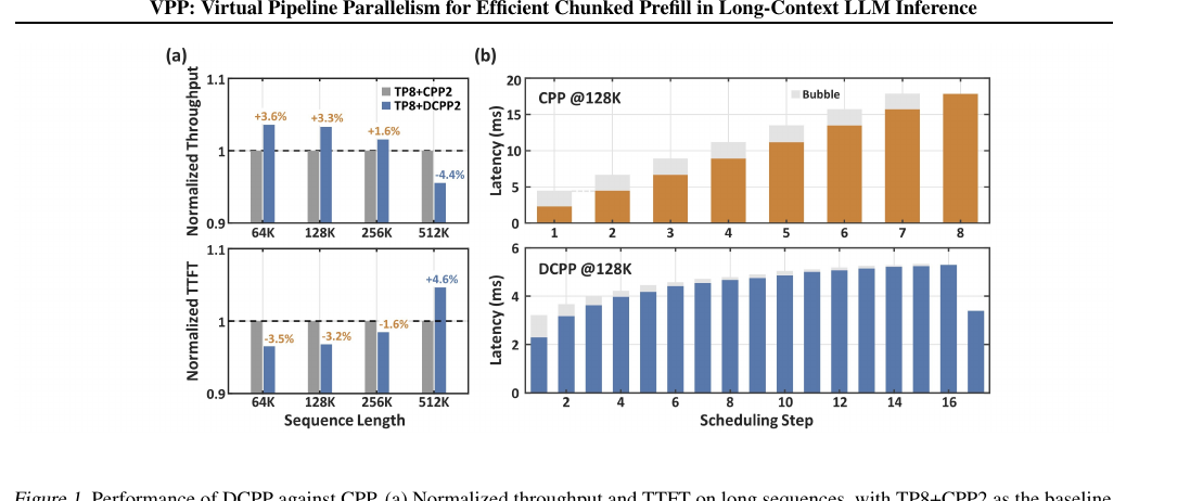
Panel (b) is the key diagnostic: CPP completes an 128K prompt in 8 scheduling steps, with per-chunk latency growing roughly linearly and visible gray “bubble” regions stacking up at later steps. DCPP completes the same prompt in 17 steps — more than twice as many — trading fragmentation for a flatter per-chunk latency profile.

At the 512K point, where the DCPP-optimal chunk budget is 24K, the paper’s profiler traces show:

	CPP (s)	DCPP (s)	$\Delta$ (s)	$\Delta$/CPP
Computing	252.59	279.07	+26.48	+10.48%
Bubble	38.64	20.47	-18.17	-47.03%
Exposed Comm.	16.67	22.68	+6.01	+36.05%
Total	307.90	322.22	+14.32	+4.65%

DCPP does deliver on its promise — bubble time drops 47%, saving 18.17s. But this saving is entirely eaten (and then some) by a 10.5% increase in computation time (smaller chunks run less efficiently as fused kernels) and a 36.1% increase in exposed communication (more chunk boundaries mean more send/recv events). The paper’s summary insight, worth internalizing: DCPP trades scheduling overhead for load-balancing gains, and this trade becomes unfavorable precisely as sequences get long — which is exactly the regime long-context serving cares most about.

Design-choice discussion. Why not just tune DCPP’s chunk-size granularity to reduce the fragmentation cost? The paper doesn’t explicitly rule this out, but the tension is structural: DCPP’s entire mechanism is fine-grained resizing — if you coarsen it to reduce fragmentation, you lose the balancing precision that was the point. There’s no free parameter that escapes this trade-off within DCPP’s own design space; it’s baked into “shrink chunks to equalize latency.”

4. VPP: Design and Implementation (§5)

4.1 The core insight

The paper observes that the per-chunk latency growth under causal attention with fixed chunk size is not arbitrary noise — it is approximately linear in the chunk index. If we denote the per-stage latency of chunk $C_k$ (the $k$-th chunk, 0-indexed) as $\tau_k$, the empirical regularity is:

$$\tau_k = (k+1)t, \tag{2}$$

where $t$ is the per-stage latency of the very first chunk $C_0$. This holds when attention dominates the per-chunk cost and MoE routing is expert-parallel (so MoE overhead is a roughly fixed additive term, not something that itself scales with $k$).

Instead of eliminating this heterogeneity (DCPP’s approach), VPP’s insight is to exploit its predictability to construct a pipeline schedule where the extra work of later chunks is deliberately matched by extra parallel work elsewhere in the pipeline, so nothing sits idle.

4.2 VPP: V-shaped pipeline scheduling (§5.1)

Consider the simplest concrete instance: two physical pipeline ranks, $pp_0$ and $pp_1$. The model’s layers are partitioned into four virtual stages $s_0, s_1, s_2, s_3$. Instead of mapping stage $i$ to rank $i \bmod 2$ in the conventional unidirectional way, VPP places the two boundary stages ($s_0, s_3$) on $pp_0$, and the two middle stages ($s_1, s_2$) on $pp_1$.

A chunk $C_k$ then traverses the ranks in a “fold-back” pattern:

$$s_0(pp_0) \rightarrow s_1(pp_1) \rightarrow s_2(pp_1) \rightarrow s_3(pp_0).$$

$pp_0$ starts the chunk, hands it to $pp_1$ which runs both middle stages back-to-back, then hands it back to $pp_0$ for the final stage. Because the chunk goes rank$\to$rank$\to$rank and back, the trajectory forms a visual “V” — hence Virtual Pipeline Parallelism’s name (also echoing “virtual pipeline” scheduling from training-time interleaved pipelines, but applied here to a fold-back layout rather than interleaved micro-batches).

Why does this balance the pipeline? Here’s the derivation, spelled out step by step. While $pp_1$ is busy running the two middle stages of chunk $C_k$, its total occupied time is approximately

$$2\tau_k = 2(k+1)t. \tag{3a}$$

During that same time window, $pp_0$ is not idle — it has two pieces of ready work available: finishing the exit stage of the previous chunk, $s_3/C_{k-1}$, whose latency is $\tau_{k-1} = kt$, and starting the entry stage of the next chunk, $s_0/C_{k+1}$, whose latency is $\tau_{k+1} = (k+2)t$. Adding these:

$$\tau_{k-1} + \tau_{k+1} = kt + (k+2)t = 2(k+1)t = 2\tau_k. \tag{3b}$$

This is the algebraic heart of the whole method: the combined workload $pp_0$ can do while $pp_1$ is busy on $C_k$‘s middle stages exactly matches $pp_1$‘s occupied time, for any $k$, as long as the linear-$\tau_k$ assumption (Eq. 2) holds. In other words, the growing cost of later chunks isn’t erased — it’s rescheduled so that both ranks are always doing something useful, rather than one rank waiting on the other.

The boundary case is $C_0$: while $pp_1$ handles its two middle stages ($2\tau_0 = 2t$), $pp_0$ only has $s_0/C_1$ available (latency $\tau_1 = 2t$) since there’s no $C_{-1}$ — the numbers still match by coincidence of the linear formula, so even the very first chunk doesn’t introduce an imbalance.

Numbered pseudocode for the V-shaped scheduling logic:

Algorithm 1: V-shaped Virtual-Stage Scheduling (two-rank case)
Input: chunk sequence C_0, ..., C_{N-1}; virtual stages s_0, s_1, s_2, s_3
        mapped to physical ranks pp_0 (s_0, s_3) and pp_1 (s_1, s_2)
Output: per-rank execution schedule

1:  for k = 0 to N-1:
2:      pp_0 executes s_0 on chunk C_k         # entry stage
3:      pp_0 sends activation(s_0, C_k) to pp_1
4:      pp_1 executes s_1 on chunk C_k
5:      pp_1 executes s_2 on chunk C_k          # two middle stages, back-to-back
6:      pp_1 sends activation(s_2, C_k) to pp_0
7:      pp_0 executes s_3 on chunk C_k          # exit stage
8:      # Note: while pp_1 runs lines 4-5 for C_k, pp_0 concurrently
9:      #       executes line 7 for C_{k-1} and line 2 for C_{k+1},
10:     #       filling what would otherwise be idle time
11: end for

Concrete numerical walk-through. Suppose $t = 1$ (arbitrary latency unit) and we’re at chunk $k=3$. Then $\tau_3 = 4$: $pp_1$ spends $2\tau_3 = 8$ units running $s_1/C_3$ and $s_2/C_3$. Meanwhile $pp_0$ runs $s_3/C_2$ (latency $\tau_2 = 3$) and $s_0/C_4$ (latency $\tau_4 = 5$), totalling $3 + 5 = 8$ units — an exact match. This is precisely Eq. (3b) instantiated: $\tau_{k-1} + \tau_{k+1} = 3 + 5 = 8 = 2 \times 4 = 2\tau_k$.

Where this breaks down (design boundary, stated explicitly by the authors): the whole derivation leans on the linear-$\tau_k$ regime holding. If attention stops being the dominant cost component (e.g., a very sparse-attention model where attention FLOPs grow sub-linearly with context, or if expert-parallelism is disabled so MoE routing/communication becomes a growing rather than fixed cost), the equality in Eq. (3b) no longer holds exactly, and steady-state bubbles can reappear. The paper later confirms this experimentally with GLM-5.2’s DSA (sparse) attention — more on that in §7.

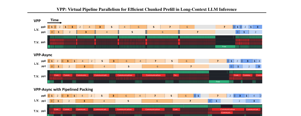
Figure 2 visualizes the resulting scheduling timeline compared to plain CPP.

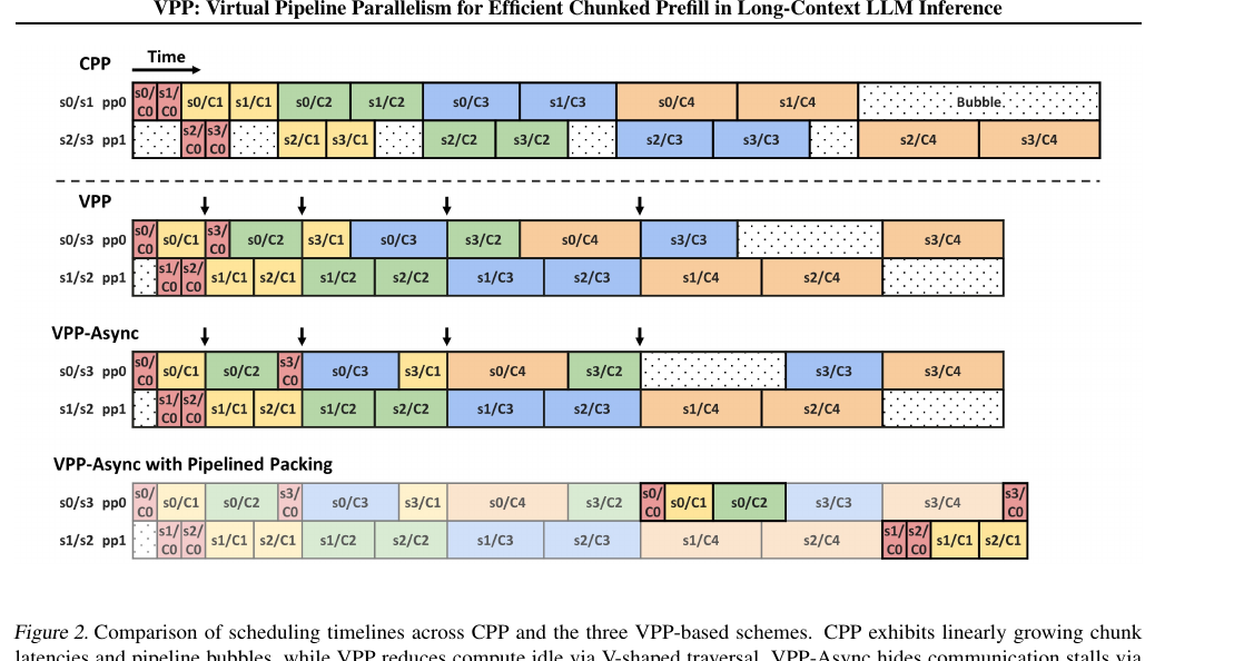
Notice in the CPP row how bubbles (dotted regions) accumulate and grow toward the end of the sequence — this is the imbalance visualized directly. In the VPP row, the fold-back layout keeps both ranks continuously busy for almost the entire duration, with only a residual “drain” bubble at the tail.

4.3 Two remaining inefficiencies, and why they matter

Even with the V-shaped layout solving the compute-balance problem, two inefficiencies remain, both visible as gaps in the VPP row of Figure 2:

1. Every arrow between ranks in Figure 2 represents a synchronous, blocking send/recv. The receiver must wait for the full activation transfer before starting compute — communication sits directly on the critical path.
2. The final chunks of a request inevitably leave one rank idle once its own work runs out but the other rank is still finishing up — a drain bubble that’s inherent to any pipelined execution of a single, finite request.

VPP addresses these with two further optimizations, described next.

4.4 VPP-Async: communication-computation overlap (§5.2)

At a handoff between, say, $C_1$ and $C_2$, the naive V-shaped scheme has $pp_0$ send $s_0/C_2$ forward to $pp_1$ while simultaneously $pp_1$ sends $s_2/C_1$ back to $pp_0$. Both directions block: each rank waits for its respective inbound transfer before it can proceed, even though there’s no fundamental data dependency forcing this — the stall is purely an artifact of operation ordering.

The fix: once the required prefix KV cache is locally available, a rank can reorder its own instruction stream to avoid issuing both directions of communication simultaneously. Concretely, VPP-Async swaps the order in which $pp_0$ issues the tail-stage computation of $C_{k-1}$ ($s_3/C_{k-1}$) and the head-stage computation of $C_{k+1}$ ($s_0/C_{k+1}$), so that each communication event is issued while the peer rank is busy with useful compute rather than also trying to communicate at the exact same instant. This is implemented with two alternating HCCL communication groups exchanging activations via point-to-point send/recv, specifically to avoid deadlocks that bidirectional transfers on a single group could cause.

Design-choice discussion: why reordering rather than, say, just making communication itself asynchronous/non-blocking at the framework level? The paper’s approach is cheaper to implement correctly (no need to redesign the whole activation-passing API) and directly targets the root cause (ordering), rather than papering over a scheduling problem with more asynchrony primitives that could introduce new race conditions. The trade-off: it requires the scheduler to know, ahead of time, which chunk pairs will collide, which ties the implementation to the specific V-shaped layout rather than being a general-purpose async communication library.

4.5 VPP-Async with Pipelined Packing: cross-request bubble compression (§5.3)

Even with intra-request stalls hidden, the tail of any single request leaves a genuine drain bubble: the last couple of chunks ($C_{N-2}, C_{N-1}$) finish their V-traversal, and one rank runs out of work for this request while waiting for the request to fully complete.

But in a real serving system, requests arrive continuously. VPP’s third optimization packs the leading chunks of the next request $R'$ into the tail drain-bubble window of the current request $R$. The paper computes that this drain window has duration approximately $(N+1)t$ — and since the early chunks of any request have the lowest per-chunk latency ($\tau \approx t$, from Eq. 2 with small $k$), they are exactly the right size to slot into a shrinking tail window without further growing it.

Numbered pseudocode:

Algorithm 2: Pipelined Packing Across Requests
Input: current request R with chunks C_0...C_{N-1} nearing completion;
        next queued request R' with chunks C'_0, C'_1, ...
Output: packed schedule filling R's drain bubble with R''s leading chunks

1:  while R has chunks remaining in its V-traversal:
2:      schedule R's next chunk normally (Algorithm 1, steps 1-11)
3:  end while
4:  # R enters drain phase: only its final stage-3 completions remain
5:  drain_window_estimate <- (N + 1) * t
6:  j <- 0
7:  while drain_window_estimate not exhausted AND R' has chunks left:
8:      schedule C'_j into the idle rank slot(s) freed by R's drain
9:      j <- j + 1
10:     drain_window_estimate <- drain_window_estimate - tau(C'_j)
11: end while
12: once R fully completes, resume normal V-shaped scheduling
     for the remainder of R' (and subsequent requests)

This is a dual-queue scheduler: batches waiting for their initial virtual-stage traversal sit in one queue; batches that have passed the fold point migrate to a continuation queue for final-stage execution and sampling. The scheduler keeps one extra in-flight batch and uses asynchronous task handles so this bookkeeping never blocks the main scheduling loop.

4.6 Design-choice summary table

To make the accumulated design decisions easy to scan, here is a consolidated view of every non-trivial choice VPP makes, the obvious alternative, and where each choice’s assumptions could fail:

Design choice	Why it works	Obvious alternative	Where it fails
Fixed chunk size + fold-back layout	Exploits predictable linear $\tau_k$ growth (Eq. 2) instead of fighting it	Dynamic chunk resizing (DCPP)	Breaks down if $\tau_k$ is not linear (e.g., sparse attention, §7.5)
V-shaped (boundary-stage / middle-stage) rank assignment	Algebraically balances $pp_0$ and $pp_1$ workload for any $k$ (Eq. 3b)	Conventional unidirectional stage-to-rank mapping	Requires exactly matching stage counts to ranks; harder to generalize to odd numbers of stages or ranks
Synchronous send/recv reordering (VPP-Async)	Removes exposed communication without new async primitives	Framework-level fully asynchronous communication API	Requires the scheduler to know chunk-pair collision patterns ahead of time; ties implementation to this specific layout
Cross-request pipelined packing	Reuses drain-bubble idle time productively	Simply accept the drain bubble as unavoidable pipeline overhead	Needs a next request to be queued and ready; provides no benefit under low-concurrency / bursty-arrival regimes
24K as empirically-preferred chunk size	Leaves an uneven remainder chunk that shrinks the tail bubble	Evenly-divisible chunk sizes (8K/16K/32K)	At very short sequences (64K on DeepSeek/GLM) the pipeline never reaches steady state, reversing the preference

4.7 A second numerical walk-through: the drain-packing arithmetic

It’s worth grounding Algorithm 2’s abstract $(N+1)t$ estimate with numbers. Suppose a request $R$ has $N = 8$ chunks and $t = 1$ (arbitrary latency unit, matching the earlier §4.2 example). The drain window duration estimate is $(8+1) \times 1 = 9$ units. Now suppose the next queued request $R'$ has chunks with the same linear latency law, $\tau'_j = (j+1)t$. Packing greedily from $j=0$:

$$\tau'_0 + \tau'_1 + \tau'_2 = 1 + 2 + 3 = 6 \le 9, \tag{4a}$$

so the first three chunks of $R'$ fit inside the 9-unit drain window with 3 units to spare (not quite enough for a fourth chunk, since $\tau'_3 = 4 > 3$ remaining). This directly illustrates why the paper packs the leading chunks specifically — they are cheapest, by construction of the same linear law that created the drain bubble’s size in the first place. If the scheduler instead tried to pack later, more expensive chunks of $R'$ first (the obvious naive alternative), it would either overflow the drain window and reintroduce a bubble on $R'$‘s own critical path, or under-fill the window and leave idle time unused — so the FIFO/earliest-chunk-first packing order is not an arbitrary implementation detail but a direct consequence of the same linear-latency structure the whole method is built on.

5. Implementation Details (§5.4)

VPP is implemented on top of vLLM-Ascend using PyTorch and HCCL, targeting Huawei Ascend 910C NPUs. A few implementation specifics worth calling out because they affect how transferable the idea is to other stacks:

• Control-plane logic (virtual-stage scheduler, fold-back layer assignment, per-batch pipeline state machine) is pure Python; the actual attention/MoE compute kernels are reused unmodified from upstream vLLM-Ascend. This is a meaningful design choice — VPP is a scheduling layer, not a new kernel, which is why it can be a single feature flag (enabled/disabled) without touching the compute path.
• The fold-back topology generalizes beyond 2 ranks / 4 stages: “the first half of virtual stages traverse forward across ranks and the second half traverse backward,” with fold points (where two consecutive virtual stages land on the same physical device) requiring zero inter-device communication — a nice free efficiency win at the fold point itself.
• The implementation supports uneven layer partitioning — i.e., you don’t have to give every virtual stage exactly the same number of transformer layers; this is a knob for balancing memory/compute beyond the pure latency-scheduling problem addressed above.

Design-choice discussion — why vLLM-Ascend specifically, and what does this mean for portability? The paper doesn’t claim VPP is Ascend-specific in its algorithm — the derivation in §4.2 is architecture-agnostic — but the implementation leans on Ascend-specific primitives (HCCL communication groups, CANN toolkit, torch_npu). A GPU port would need to swap HCCL for NCCL and re-validate the async communication-group deadlock-avoidance logic, but there’s nothing in the core scheduling algorithm that’s inherently NPU-specific. The obvious alternative — implementing this purely as a vLLM scheduler plugin independent of hardware backend — would be architecturally cleaner but the paper doesn’t attempt it, presumably because the deadline/production pressure was to ship on Ascend hardware specifically (Huawei is the primary affiliation).

6. Experimental Setup (§6.1)

• Hardware: Huawei Atlas 900 A3 SuperPoD, 16 Ascend 910C NPUs (64GB HBM each), HCCS interconnect, all collectives via HCCL.
• Software: PyTorch v2.10.0 + torch_npu, CANN v8.3, vLLM v0.23.0 with vLLM-Ascend v0.23.0.
• Models: three MoE-based LLMs spanning different attention mechanisms — Qwen3-Coder-30B-A3B-Instruct (30.5B total / 3.3B active, 128 experts, GQA attention), DeepSeek-V3.1-Terminus (671B total / 37B active, 256 experts, MLA attention), and GLM-5.2 (744B total / 40B active, 256 experts, MLA + DSA sparse attention).
• Baselines: TP8+CPP2 (chunked prefill pipeline parallelism, static chunks), TP8+DCPP2 (dynamic chunk resizing, vLLM-Ascend’s recommended settings: minimum chunk 4096 tokens, smoothing factor 1.0), and TP8+VPP2 (the proposed scheme). All use 8-way tensor parallelism plus 2-way pipeline parallelism.
• Workloads: (1) short: 100 concurrent requests at 4K/8K/16K tokens; (2) long: single request at a time, 64K to 1M tokens; (3) mixed: 500 requests synthesized from GSM8K with lengths from 7 to 122,710 tokens (mean $\approx$22.5K, median $\approx$10K, p90 $\approx$64K), concurrency 16.
• Metrics: throughput (tokens/s) and TTFT (s), each averaged over 4 runs per (strategy, workload, chunk-budget) combination, sweeping chunk size over {8K, 16K, 24K, 32K} and reporting the best-performing budget for each strategy.

Reproducibility note: the implementation is open-sourced at github.com/RookieCoder-Camera/vllm-ascend/tree/vpp-dev, which is a meaningful plus for reproducibility — but note this is a development branch, not a tagged release, and the paper does not report specific commit hashes or exact software versions beyond the major version numbers listed above; anyone trying to reproduce exact numbers should expect some variance from branch drift.

7. Results

7.1 Long sequences — where VPP is designed to shine

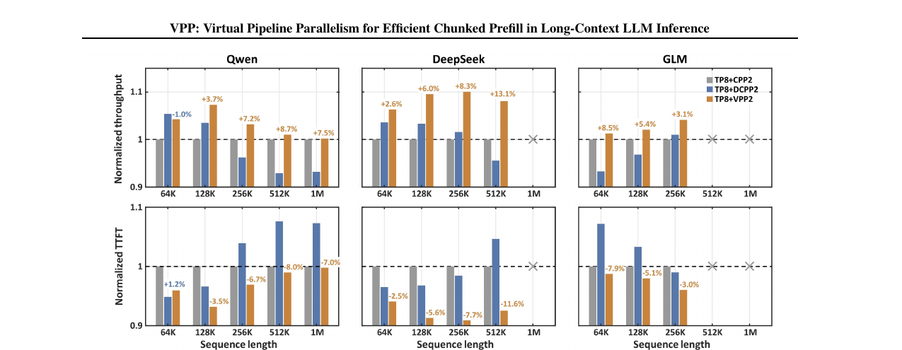
VPP outperforms both CPP and DCPP in nearly every configuration. Compared with CPP: up to 7.3% (Qwen), 10.0% (DeepSeek), 4.1% (GLM) throughput improvement, with comparable TTFT reductions. Compared with DCPP: the advantage generally increases with sequence length on Qwen and DeepSeek — 3.7%–8.7% on Qwen (128K–512K) and 2.6%–13.1% on DeepSeek (64K–512K). This monotonic-with-length trend is the paper’s central empirical claim vindicated: the longer the sequence, the more DCPP’s fragmentation overhead accumulates, and the more room VPP has to win by avoiding that fragmentation entirely.

GLM is the interesting exception: VPP’s gain over DCPP peaks at 64K (8.5%) and narrows at longer lengths, rather than growing. The paper attributes this to GLM’s DSA (sparse) attention breaking the linear-$\tau_k$ assumption — this is directly the boundary condition flagged in §4.2, now showing up empirically. We’ll come back to this.

7.2 Mixed-length sequences — the realistic serving scenario

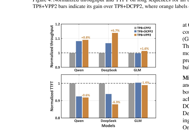
On Qwen: +9.0% over CPP, +0.8% over DCPP. On DeepSeek (VPP’s best case): +13.8% over CPP, +6.7% over DCPP. On GLM: a more modest +1.3%–1.6% over both baselines. This is arguably the most practically relevant result set, since production serving traffic is rarely uniformly-long or uniformly-short — it’s a heavy-tailed mix, and VPP holds its advantage across that mix without needing to know in advance which regime a given request falls into (a real strength versus a hypothetical scheme that requires online mode-switching).

7.3 Short sequences — checking for regressions

The paper reports (§6.2, no dedicated figure reproduced here beyond the source paper’s Fig.3) that VPP shows “almost no regression” against DCPP on short (4K–16K) sequences — comparable on Qwen and GLM, with VPP’s largest advantage on DeepSeek reaching 10.8% at 4K chunk size. Compared to CPP, VPP degrades by up to 6.8% on Qwen at short lengths, attributed to Qwen’s small active parameter count (3.3B) making scheduling overhead proportionally larger relative to compute — i.e., there isn’t enough real work to amortize VPP’s own bookkeeping when the model itself is cheap to run. This is an honest negative result the authors report rather than hide, which is good practice, though as discussed in §9 below it’s also somewhat underexplored.

7.4 Source-of-gains breakdown (§6.3, Table 2)

To understand where VPP’s TTFT improvement actually comes from (rather than just reporting an aggregate number), the authors profile the DeepSeek-V3.1 512K workload and decompose the difference into computation, bubble, and exposed-communication components.

	DCPP (s)	VPP (s)	$\Delta$ (s)	$\Delta$/DCPP
(a) End-to-end
Computation	279.07	250.84	-28.23	-10.11%
Bubble	20.47	0.39	-20.07	-98.04%
Exposed Comm.	22.68	30.63	+7.95	+35.05%
Net (profiler)			-40.36	-12.53%
(b) Computation detail
Attention	228.13	233.08	+4.96	+2.17%
Slice	22.90	5.18	-17.72	-77.38%
MatMulV3	13.06	2.54	-10.52	-80.55%
(c) Bubble detail
Free	18.61	0.39	-18.22	-97.90%
Launch stall	1.85	0.00036	-1.85	-99.98%

A few things worth pausing on here:

1. VPP’s attention kernel time is actually longer, not shorter, than DCPP’s (+2.17%). This is an important, non-obvious result: VPP’s win does not come from computing attention faster. It comes from fewer, larger attention invocations — DCPP issues more, smaller attention calls (matching its many small chunks), and while each individual call is cheap, the aggregate kernel-launch and scheduling overhead (captured mostly in “Slice” and “MatMulV3,” which drop 77% and 81% respectively) dominates. This distinction matters: it tells you VPP is not a “faster kernel” story, it’s an “eliminate fragmentation” story, consistent with the paper’s own framing.
2. Bubble reduction is almost total (98.04%), which is the headline number the abstract leads with.
3. Exposed communication actually goes up by 35% under VPP — this is the honest cost of the approach. The paper explains this as mostly additional AllGather auxiliary overhead: VPP issues 4.58× fewer AllGather calls, but each call’s average latency increases 11×, netting a 39.7% (5.27s) increase in AllGather overhead specifically. However, the overlap ratio — how much of this communication hides behind useful computation — jumps from 0.05% to 51.75%, which is why the net effect is still a win despite the raw communication time going up. This is a genuinely interesting systems lesson: raw metric regressions (more communication time) can still net out to a win if overlap improves enough, and a superficial read of “communication went up 35%” without this context would be misleading.

7.5 Impact of sparse attention (a genuine limitation surfaced by the authors)

The paper explicitly investigates GLM-5.2’s DSA (sparse) attention at 128K tokens to understand why VPP’s advantage narrows for this model at longer contexts. Because DSA reduces the growth rate of attention cost with accumulated prefix length, the near-linear $\tau_k$ scaling VPP’s entire derivation depends on no longer strictly holds: early chunks still benefit from the V-shaped interleaving, but “scheduling efficiency gradually degrades” for later chunks, and bubbles start reappearing. The authors are upfront that VPP “still achieves positive gains… at contexts below 512K,” but do not report numbers at or above 512K for GLM in the long-sequence sweep (Figure 4’s GLM panel shows an “X” marker at 512K/1M, meaning no data reported) — this gap is worth flagging (see §9).

7.6 Ablation of VPP variants (§6.4)

Using a 256K-token DeepSeek workload, 32K chunk size, three concurrent requests, the paper isolates each optimization’s individual contribution:

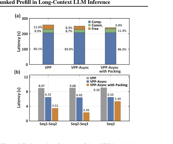
• Vanilla VPP → VPP-Async: 3.13% end-to-end latency reduction, driven by cutting non-overlapped communication by 48% and raising the communication overlap ratio from 0.02% to 54.03%.
• VPP-Async → VPP-Async with Pipelined Packing: a further reduction to 6.89% total (over vanilla VPP), driven by cutting cross-request bubble latency by 33.2%.
• Compute time itself varies by at most 0.82s (0.42%) across all three variants — confirming (as in §7.4) that essentially all of the gain across variants is a scheduling effect, not a compute-efficiency effect.

The bubble ratio numbers tell the same story quantitatively: 11.0% (vanilla VPP) → 8.3% (VPP-Async) → 2.4% (VPP-Async with Packing), each optimization chipping away at a specific, previously-identified source of idle time.

7.7 Chunk-size sensitivity (§6.4, Figure 8 in the source paper)

Sweeping chunk size from 8K to 32K across sequence lengths 64K–1M reveals a counter-intuitive result: 24K performs best in most configurations, not because it’s some universally optimal token count, but because it does not divide sequences evenly — the final, smaller “remainder” chunk ends up executing during the pipeline drain phase, where its computation and communication overlap with preceding chunks, shrinking what would otherwise be a larger tail bubble under an evenly-divisible chunk size. The exception: at 64K sequence length on DeepSeek and GLM, throughput drops monotonically as chunk size shrinks, because with only a few chunks total, the pipeline never reaches a steady state, and smaller chunks just directly shorten the (already-dominant) tail bubble rather than providing balancing benefit.

8. Reproducibility Notes

What’s disclosed: model names/sizes, hardware (16× Ascend 910C, 64GB HBM), software stack versions (PyTorch 2.10.0, CANN 8.3, vLLM/vLLM-Ascend 0.23.0), parallelism config (TP8 + PP2), chunk-size sweep range, workload construction (GSM8K-derived mixed lengths, concrete percentile statistics), and an open-source implementation branch.

What’s not disclosed or left ambiguous, which would matter for exact reproduction:

• Exact HCCL communication-group configuration parameters (buffer sizes, timeout settings) for the async communication-group swap described in §5.2/§5.4.
• The precise heuristic or threshold used to decide the size of the “packing window” in Algorithm 2 beyond the approximate $(N+1)t$ estimate — is this a fixed constant, a runtime-estimated value, or adaptively tuned per request? The paper describes the intent but not the exact online estimation procedure.
• DCPP’s own internal cost-estimation/calibration hyperparameters (the paper uses “vLLM-Ascend’s recommended settings” without listing the underlying online estimator’s parameters), which somewhat limits independent verification of the DCPP baseline numbers specifically.
• Random seeds or run-to-run variance beyond “averaged over 4 runs” — no standard deviations or confidence intervals are reported for any of the throughput/TTFT numbers.

9. Limitations, What the Authors Understate, and Critical Analysis

(a) Weaknesses and flaws specific to this paper.

1. No standard deviation or variance reporting anywhere. Every single number in this paper — the 13.1% headline gain, the 98.0% bubble reduction, the ablation deltas — is reported as a bare mean over 4 runs. For a systems paper making percentage-point claims in the single digits in several places (e.g., GLM’s 1.3%–1.6% mixed-workload gains), the absence of any variance information makes it impossible to judge whether these smaller gains are statistically meaningful or within noise. This is a straightforward, fixable omission that meaningfully weakens confidence in the more marginal results.
2. The GLM/DSA limitation is reported but not fully characterized. The authors tell us qualitatively that VPP’s advantage narrows with sparse attention and stop reporting numbers past 512K for GLM, but they don’t quantify how much the linear-$\tau_k$ assumption breaks down (e.g., what’s the actual measured $\tau_k$ growth curve for DSA vs. dense attention?), nor do they attempt any fix or adaptive mechanism for this case within the current paper — it’s flagged purely as future work. Given that sparse attention is an increasingly common design choice in frontier long-context models (this exact trend is why GLM-5.2 uses DSA in the first place), this is a real gap in a paper whose main selling point is long-context serving.
3. Only one specific two-rank, four-virtual-stage instantiation is evaluated in depth. All experiments use TP8+“VPP2,” i.e., 2-way pipeline parallelism. The core derivation in §4.2 is stated in terms of a 2-rank / 4-stage case; the paper claims the fold-back topology “generalizes” to deeper pipelines with more ranks, but no experimental results are shown for, say, 4-way or 8-way pipeline parallelism, where the combinatorics of matching cross-rank workloads (Eq. 3b’s clean algebraic match) would presumably become considerably harder to maintain, especially as you add more virtual stages with more varied per-stage costs.

(b) Limitations the authors understate or omit.

1. The short-sequence Qwen regression (up to -6.8% vs. CPP) is explained with a single hand-wavy sentence (“smaller active parameter count… makes scheduling overhead less amortizable”) without any breakdown analogous to Table 2’s decomposition for the long-sequence case. Given that Table 2’s methodology (computation/bubble/communication decomposition) was clearly available to the authors and used elsewhere in the paper, its absence here specifically for a negative result reads as an editorial choice to under-invest analytical effort where the news is bad.
2. No discussion of scheduler complexity or maintenance cost. VPP introduces a dual-queue scheduler, a fold-back layer-assignment mechanism, cross-rank reordering logic, and cross-request packing heuristics — this is meaningfully more complex than either CPP (trivial round-robin through stages) or even DCPP (whose complexity is at least concentrated in a single, well-understood “estimate cost, resize chunk” loop). The paper doesn’t discuss engineering/maintenance overhead, debuggability, or how VPP interacts with other production concerns like request preemption, priority scheduling, or SLO-aware admission control that a real serving system also has to handle simultaneously.
3. The paper doesn’t discuss memory implications of the fold-back layout. Having chunks traverse ranks and come back means activations for in-flight chunks may need to be buffered longer, and the in-flight-batch bookkeeping (one extra batch, per §5.4) has some memory footprint that isn’t quantified anywhere in the paper.

(c) Concrete, specific improvement suggestions.

1. Report variance/confidence intervals (at minimum standard deviation across the 4 runs) for every throughput/TTFT number, especially the smaller GLM mixed-workload gains where the signal-to-noise ratio is least clear.
2. Extend the Table 2-style computation/bubble/communication breakdown to the short-sequence Qwen regression case, so readers can see concretely whether the loss is dominated by scheduler overhead, communication, or something else — right now it’s asserted rather than shown.
3. Provide at least one experimental data point with pipeline-parallel degree > 2 (e.g., TP4+VPP4 or similar), even at smaller scale, to substantiate the “generalizes to deeper pipelines” claim empirically rather than leaving it purely as an architectural assertion.
4. For the DSA/sparse-attention limitation, report the actual measured $\tau_k$-vs-$k$ curve for GLM at 512K/1M and compare it quantitatively against the linear model in Eq. (2) — this would let readers (and the authors, in follow-up work) see exactly how much slack exists before a corrective mechanism (e.g., an adaptive fold-point recalibration) becomes necessary.

9b. Comparison with Related Pipeline-Balancing Work

It’s worth situating VPP precisely against the two related-work threads the paper itself cites (§3), since the distinctions are easy to blur:

• gLLM (token throttling): balances pipeline micro-batches primarily by token count, without explicitly modeling context-dependent attention cost. This means gLLM’s balancing signal is a proxy (token count) for the real cost driver (accumulated KV-cache length), whereas VPP’s Eq. (2) models the actual latency growth directly. The trade-off: gLLM’s proxy is simpler to compute online, but systematically mis-estimates cost for exactly the causal-attention regime VPP targets.
• TeraPipe / Seq1F1B (training-time token-level sequence partitioning): these formulate non-uniform chunk-boundary search as an optimization problem (dynamic programming in TeraPipe’s case) to balance micro-batch execution time — conceptually the training-time analogue of DCPP. Both keep the DCPP-style philosophy of resizing to balance, rather than VPP’s philosophy of fixing size and reshaping layout. Since these methods target training (where micro-batches repeat identically across many training steps, making runtime calibration cheap to amortize), the fragmentation-overhead argument against dynamic resizing is weaker there than in VPP’s inference-serving setting, where each prefill request is typically unique and calibration cost cannot be amortized across repeated identical batches.
• SGLang / vLLM-Ascake’s own DCPP implementations: both employ runtime profiling and online calibration to predict chunk latency and dynamically adjust boundaries — this is precisely the class of method VPP’s motivating measurement (§4) is empirically comparing against and outperforming at long sequence lengths.

The throughline: every prior approach treats chunk-latency heterogeneity as something to be removed; VPP is the first in this specific lineage to treat it as a known, exploitable structural property of the workload and design the pipeline layout around it directly.

10. Conclusion

VPP is a clean example of a systems paper that wins by changing where the imbalance is absorbed rather than trying to eliminate the imbalance’s root cause. The observation that fixed-chunk-size attention cost grows near-linearly and predictably under causal masking is not new — DCPP is implicitly built on the same observation — but VPP’s insight is that this predictability can be exploited by pipeline layout design (V-shaped fold-back scheduling) instead of by chunk resizing, and that the latter’s fragmentation cost is what actually dominates at long context lengths. The headline number — 98.0% bubble-ratio reduction and up to 13.1% throughput improvement over the existing production-grade DCPP baseline on a real 512K-token DeepSeek-V3.1 workload — is a substantial, credible systems contribution, backed by a genuinely careful multi-level breakdown (computation vs. bubble vs. communication) that avoids the common trap of reporting only aggregate numbers. The paper’s own honesty about where the method’s core assumption (linear per-chunk latency growth) breaks down — specifically for sparse-attention models like GLM-5.2’s DSA — is a good sign of scientific care, even though (per §9) that limitation deserves a more quantitative treatment than it currently gets. If you’re building or maintaining a long-context LLM serving stack with pipeline parallelism, this paper is worth reading closely for the V-shaped scheduling idea itself, independent of whether you’re on Ascend or GPU hardware — the core algebra in Eq. (2)–(3b) is hardware-agnostic and directly portable.