LowRankArena: What Happens When You Force SVD Compression Papers to Play by the Same Rules

Review date: 2026-08-28 | Author: Zhongzhu Zhou Paper reviewed: LowRankArena: A Standardized Evaluation Platform for SVD-Based LLM Compression Paper authors: Zishan Shao, Lixun Zhang, Kangning Cui, Wenhao Wu, Jinhee Kim, Yixiao Wang, Ting Jiang, Hancheng Ye, Qinsi Wang, Fan Yang, Danyang Zhuo, Yiran Chen, Hai Li (Duke University, Wake Forest University) arXiv: 2608.26389 Venue/Status: arXiv preprint, submitted 26 Aug 2026

Why This Paper Matters

Every week for the last several months in this blog series, I have reviewed a new SVD-based LLM compression method — SVD-LLM, DoBi-SVD, Swift-SVD, SigmaScale, AIR, LACE-SVD, SVD-Surgeon, and more — and every single one of these papers reported a table where their method beats the previous state of the art. If you only read these papers in isolation, you would conclude that the field has made continuous, monotonic progress: each new SVD variant is strictly better than the last.

LowRankArena is the paper that finally asks the uncomfortable question underneath that pattern: compared under whose rules? Different papers use different LLaMA checkpoints, different keep-ratio definitions, different calibration sets, different subsets of benchmark tasks, and — critically — some papers quietly bundle mixed-precision quantization or weight remapping into what they call “low-rank compression,” making it impossible to tell whether a reported win comes from the SVD algorithm itself or from an auxiliary trick riding along with it.

This is not a new algorithm paper. It is an audit paper, and it belongs to a small but important genre: papers that don’t try to move the state of the art forward, but instead ask whether the state of the art, as currently reported, is even real. The authors built a shared evaluation harness — fixed models, fixed tasks, fixed keep-ratio budget definition, fixed inference backend — reran five representative SVD methods (ASVD, SVD-LLM, DoBi-SVD, Basis Sharing, MoDeGPT) through it, and the headline finding is sobering for anyone tracking “SOTA” in this space: there is no stable, architecture-invariant ranking. The “best” method changes depending on which backbone you test, which keep ratio you use, and which metric family (accuracy vs. perplexity) you look at.

If you have been reading this blog series and mentally building a leaderboard of “best SVD method so far,” this paper is the necessary corrective: that leaderboard, as commonly reported in the literature, may not actually exist.

Prerequisites

What SVD-based LLM compression actually does

A dense weight matrix in a transformer, say $W \in \mathbb{R}^{m \times n}$ (a linear projection inside attention or the MLP block), can always be exactly factorized via the singular value decomposition:

$$W = U \Sigma V^{\top}$$

where $U \in \mathbb{R}^{m \times m}$ and $V \in \mathbb{R}^{n \times n}$ are orthogonal, and $\Sigma \in \mathbb{R}^{m \times n}$ is diagonal with non-negative singular values sorted in decreasing order: $\sigma_1 \geq \sigma_2 \geq \dots \geq \sigma_{\min(m,n)} \geq 0$. The classical Eckart–Young theorem says that if you keep only the top $k$ singular values (and the corresponding columns of $U$ and rows of $V^{\top}$), you get the best possible rank-$k$ approximation of $W$ in Frobenius norm:

$$\hat{W}_k = U_{:,1:k} \, \Sigma_{1:k,1:k} \, V_{:,1:k}^{\top}, \qquad \| W - \hat{W}_k \|_F = \min_{\text{rank}(\hat{W}) \leq k} \| W - \hat{W} \|_F.$$

The practical appeal for LLM compression is that $\hat{W}_k$ can be stored and multiplied as two smaller matrices $A = U_{:,1:k}\Sigma_{1:k,1:k}^{1/2} \in \mathbb{R}^{m\times k}$ and $B = \Sigma_{1:k,1:k}^{1/2}V_{:,1:k}^{\top} \in \mathbb{R}^{k\times n}$, so a forward pass $y = Wx$ becomes $y = A(Bx)$, at a parameter cost of $k(m+n)$ instead of $mn$. When $k \ll \min(m,n)$, this is a large memory reduction, and — in principle — a large FLOP reduction too, since two small GEMMs (general matrix multiplies) can be cheaper than one big one.

flowchart LR
    subgraph Dense["Dense Layer: mn parameters"]
        W["W (m x n)"]
    end
    subgraph SVD["Full SVD (exact, no savings yet)"]
        U["U (m x m)"] --> S["Sigma (m x n)<br/>diagonal, sorted"] --> V["V^T (n x n)"]
    end
    subgraph LowRank["Truncated rank-k: k(m+n) parameters"]
        A["A = U[:,1:k] Sigma[1:k,1:k]^0.5<br/>(m x k)"] --> B["B = Sigma[1:k,1:k]^0.5 V[:,1:k]^T<br/>(k x n)"]
    end
    W -- "decompose" --> U
    S -- "keep top-k singular values only" --> A
    B -- "y = A(Bx) replaces y = Wx" --> Out["Forward pass output"]

Figure A (math-visualizing figure): from a dense weight matrix to its truncated low-rank factorization. The middle block is the exact, lossless SVD; the bottom block is what actually gets stored and executed after keeping only the top $k$ singular directions — this is the mechanical operation every method audited in this paper performs, they only differ in how they choose which directions matter.

The catch, and the reason there are dozens of papers on this topic instead of one, is that plain SVD on raw weights is a bad approximation of what actually matters, which is the model’s behavior, not its weights’ Frobenius-norm reconstruction error. A weight direction with a small singular value can still matter a lot if the activations flowing through it are large (activation-aware methods like ASVD and SVD-LLM correct for this), and a uniform rank budget across all layers ignores that some layers are far more compressible than others (adaptive-rank methods like MoDeGPT and Basis Sharing address this). This is why the field has accumulated so many variants: activation-aware rescaling, loss-sensitive truncation, cross-layer parameter sharing, adaptive rank allocation, and differentiable/learned truncation.

Keep ratio: the budget axis everyone reports differently

Every SVD compression paper needs to say “how much did we compress by,” and this is exactly where the comparability problem starts. LowRankArena’s fix is to nail down a single canonical definition, which we will return to below. Intuitively, “keep ratio” $r$ should mean: of all the parameters that would have been stored for these layers uncompressed, what fraction are stored after compression? A keep ratio of 60% means you’re using 60% of the original parameter budget for the compressed layers (i.e., a real 40% reduction), not that you kept 60% of the singular values (which is a different, method-dependent number, since $k(m+n)/mn$ is not the same fraction as $k / \min(m,n)$).

Perplexity vs. multiple-choice accuracy: two very different failure modes

Two evaluation metric families recur throughout this paper, and they measure genuinely different failure modes of a compressed model:

• Perplexity (PPL), computed on held-out text (WikiText-2, C4), measures how well the model’s predicted next-token distribution matches real text, averaged (geometrically) over every token. It is extremely sensitive to generative quality: even one badly mispredicted token in a stretch of otherwise fine text can spike perplexity, because $\text{PPL} = \exp\left(-\frac{1}{T}\sum_{t=1}^T \log p(x_t \mid x_{<t})\right)$ is an exponential of an average negative log-likelihood, so a few very-low-probability tokens dominate the average inside the exponent.
• Multiple-choice accuracy (MCQ), computed on tasks like BoolQ, ARC, HellaSwag, and WinoGrande, only asks the model to rank a small number of candidate completions correctly. A model can have badly degraded generative fluency and still correctly rank “yes” above “no” on a factual question, because ranking a handful of options is a far coarser signal than reproducing an entire fluent token stream.

The paper’s central empirical warning is that these two metrics can disagree sharply, and a method that looks fine on MCQ can be quietly catastrophic on PPL — meaning it would produce garbled, incoherent generations in practice even while “passing” a multiple-choice benchmark suite.

A concrete numerical intuition for why PPL is so much more punishing. Suppose a model assigns probability $p=0.5$ to the correct next token at every one of $T=100$ positions except one position where a badly compressed layer causes it to assign only $p=0.0001$ to the correct token (a 5,000x drop in confidence at that single position, plausible for a compressed model hitting an out-of-distribution activation pattern). The perplexity contribution is dominated by that one term: $-\log(0.0001) \approx 9.21$ nats versus $-\log(0.5) \approx 0.69$ nats for every other position. Averaging over $T=100$ positions, that single bad token alone contributes $9.21/100 \approx 0.092$ nats to the average — comparable to the contribution of roughly 13 additional otherwise-perfect positions being wrong. A handful of such rare, severely mispredicted tokens (exactly what aggressive low-rank truncation can produce, since it distorts the tail of the weight-direction spectrum non-uniformly) is enough to send perplexity into the hundreds or thousands, while an MCQ task that never happens to probe exactly those fragile positions would never notice.

Structured pruning as the alternative compression paradigm

Structured pruning (e.g., LLM-Pruner, SliceGPT, BlockPruner) removes entire architectural components — attention heads, rows/columns of weight matrices, or whole transformer blocks — producing a smaller dense model rather than a factorized one. The tradeoff versus SVD: pruning changes the model’s shape and cannot preserve the original interface exactly (surviving components must be stitched back together, sometimes losing information at the seams), while SVD factorization preserves each layer’s original input/output interface exactly and only changes what happens inside it. This paper treats structured pruning as a critical baseline that SVD methods should be honestly compared against on equal parameter budgets, not just against each other.

Why “theoretical FLOPs saved” does not equal “faster inference”

A GPU running an LLM inference workload passes through two very different computational regimes:

• Prefill (processing the input prompt): compute-bound. The GPU is doing a lot of matrix multiplication over many tokens at once, and reducing FLOPs (as SVD factorization nominally does) directly helps, because the bottleneck is arithmetic throughput.
• Decode (generating output tokens one at a time, autoregressively): memory-bandwidth-bound. Each step processes only one new token per sequence, so the matrix multiplies involved are “thin” (small batch dimension relative to weight size), and the actual bottleneck becomes how fast weights can be streamed from GPU memory, plus kernel-launch overhead, not how many FLOPs those weights require.

This distinction is the crux of the paper’s third and most practically important finding: an SVD method can reduce the raw parameter count and FLOPs (helping prefill) while doing nothing — or even hurting — decode-time throughput, because replacing one large, well-optimized dense GEMM with two smaller low-rank GEMMs can actually be slower under a memory-bound, kernel-launch-overhead-dominated regime, even though it does strictly less arithmetic.

The LowRankArena Platform: Design and Mechanism

Architecture overview: how the pieces fit together

Before diving into the audit that motivated the platform, it helps to see the platform’s own shape. LowRankArena is not a single script — it’s a layered system connecting method adapters, a fixed budget/task/inference specification, and a set of reporting tracks:

flowchart TB
    subgraph Input["Inputs"]
        A1[SVD Method Code<br/>ASVD / SVD-LLM / DoBi-SVD<br/>Basis Sharing / MoDeGPT]
        A2[Backbones<br/>Llama-1-7B / Llama-3.1-8B<br/>Qwen3-8B-Base]
    end
    subgraph Core["LowRankArena Core"]
        B1[Method Adapter Layer<br/>unifies calling convention]
        B2[Standardized Keep-Ratio<br/>Budget Enforcement]
        B3[Task Suite<br/>MCQ + PPL + Math/MMLU]
        B4[vLLM Inference Harness<br/>TTFT / E2E / throughput]
    end
    subgraph Output["Reporting Tracks"]
        C1[Main Leaderboard]
        C2[Literature Alignment]
        C3[Broader Evaluations]
        C4[Inference Speedups]
        C5[Feasibility Audit]
    end
    A1 --> B1
    A2 --> B1
    B1 --> B2
    B2 --> B3
    B2 --> B4
    B3 --> C1
    B3 --> C2
    B3 --> C3
    B4 --> C4
    B2 --> C5

Figure 1 (architecture overview): LowRankArena’s layered evaluation architecture. Method code and backbone checkpoints enter through a common adapter layer; the standardized keep-ratio budget and fixed task/inference specifications are then applied uniformly before results fan out into five reporting tracks.

The key structural point this diagram makes: every method passes through the same adapter, budget-enforcement, and task/inference layers before results reach any reporting track. This is precisely what makes cross-method comparison meaningful — no method gets a private evaluation path.

Data-flow: from raw method claim to standardized verdict

It also helps to see the audit as a pipeline over time — each method’s journey from “as originally published” to “as standardized here”:

flowchart LR
    P1[Original Paper<br/>self-reported ratio,<br/>own task subset] --> P2[Re-implement/Adapt<br/>under shared interface]
    P2 --> P3[Apply Standardized<br/>Keep-Ratio Formula]
    P3 --> P4[Evaluate on Fixed<br/>Task Suite]
    P3 --> P5[Serve via Shared<br/>vLLM Harness]
    P4 --> P6[Standardized<br/>Accuracy/PPL Verdict]
    P5 --> P7[Standardized<br/>Speedup Verdict]
    P6 --> P8[Compare Across<br/>Backbones/Ratios]
    P7 --> P8
    P8 --> P9[Reported Progress:<br/>Conditional, Not Universal]

Figure 2 (data-flow/pipeline diagram): from a method’s original, self-reported claim to LowRankArena’s standardized verdict. Every method loses its original, author-chosen evaluation conditions at step P2 and is re-measured identically from P3 onward — this is the step that actually removes the protocol-level confounds identified by the reviewer audit below.

The motivating audit: a systematic review of reviewer complaints

Before designing the platform, the authors did something methodologically clever and rare: instead of just asserting “prior evaluations are inconsistent” from personal experience, they systematically mined 76 public OpenReview reviewer and Area Chair notes on recent SVD-based LLM compression papers, and categorized the recurring complaints.

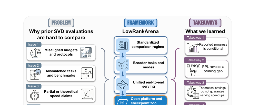
The six recurring complaint categories, ranked by frequency:

1. Narrow coverage (22.4%, 17/76): methods tested on too few model families or task versions to generalize.
2. Weak baselines (22.4%, 17/76): comparisons against outdated or poorly-tuned prior methods.
3. No end-to-end speed (21.1%, 16/76): compression ratio reported, but never validated against real inference latency/throughput.
4. Budget mismatch (17.1%, 13/76): different papers use incompatible definitions of “compression ratio,” making cross-paper comparison meaningless.
5. Mixed precision/remap (6.6%, 5/76): quantization-assisted tricks folded into the “low-rank” number without disclosure.
6. Missing artifacts (5.3%, 4/76): no released code/checkpoints, forcing later comparisons to trust self-reported numbers.

This audit is itself a nice piece of evidence-based motivation-building: rather than a rhetorical “the field lacks standardization,” it’s a quantified claim backed by a real sample of peer review text, which is a higher evidentiary bar than most systems papers bother to clear.

Design principle: separate “what changed” from “how you measured it”

LowRankArena’s core design philosophy, stated by the authors, is to fix the evaluation assumptions that most often vary across prior work, so that performance differences can be attributed to the compression method itself rather than hidden differences in evaluation setup. Concretely, it controls four axes simultaneously and independently:

1. Model coverage — which backbones are tested (legacy LLaMA-1/2-7B, and newer Llama-3.1-8B, Qwen3-8B-Base).
2. Task coverage — which benchmarks and how they’re scored (a fixed LM-Eval-Harness version, fixed prompt/shot configuration, fixed perplexity computation protocol).
3. Compression budget — the keep-ratio definition (below), applied identically to every method.
4. Inference measurement — a single shared vLLM-based serving harness with fixed hardware, precision, and request profiles.

The standardized keep-ratio formula, expanded

This is the paper’s one piece of genuine mathematical machinery, and it’s worth deriving carefully because getting it wrong is exactly the “budget mismatch” failure mode 17% of reviewers flagged. For a set of compressed linear layers $\mathcal{L}$, where layer $l$ has original weight $W_l \in \mathbb{R}^{m_l \times n_l}$ and is compressed to retained rank $k_l$:

$$r = \frac{\sum_{l \in \mathcal{L}} k_l (m_l + n_l)}{\sum_{l \in \mathcal{L}} m_l n_l}, \qquad \text{subject to} \quad \text{prec}(\hat{W}_l) = \text{prec}(W_l).$$

Let’s unpack every piece of this:

• Numerator, $k_l(m_l+n_l)$: the actual number of stored parameters for layer $l$ after low-rank factorization — recall from the SVD section above that a rank-$k_l$ factorization stores two matrices of sizes $m_l \times k_l$ and $k_l \times n_l$, totaling $k_l m_l + k_l n_l = k_l(m_l+n_l)$ scalars.
• Denominator, $m_l n_l$: the number of parameters the original dense layer would have stored.
• The ratio, summed across all compressed layers rather than computed per-layer and averaged: this matters. A parameter-weighted sum-of-numerators-over-sum-of-denominators is not the same as an average of per-layer ratios, because layers have wildly different sizes (attention projections vs. MLP up/down projections). Summing raw parameter counts first, then dividing, correctly weights the overall budget by how many actual parameters each layer contributes — exactly what you want if the goal is “total memory used,” which is the practical quantity that matters for deployment.
• The precision constraint, $\text{prec}(\hat{W}_l) = \text{prec}(W_l)$: this is the subtle, easy-to-miss clause that directly targets the “mixed precision/remap” complaint category. It says: the compressed weight must be stored at the same numerical precision (e.g., FP16 stays FP16) as the original. Without this constraint, a method could quietly compress “further” by also quantizing to INT8 or INT4 alongside the rank reduction, and then report the combined ratio as if it were purely a low-rank saving. By pinning precision equal, the formula isolates the low-rank effect from the quantization effect — these are orthogonal compression axes, and conflating them (as 6.6% of the reviewer sample flagged) makes it impossible to know which lever actually produced the reported gain.

Design choice discussion — why this specific normalization, and where it can still mislead. The obvious alternative would be to report keep ratio as a simple rank fraction, $k_l / \min(m_l, n_l)$, averaged across layers. This is simpler to compute but has two flaws the paper’s chosen formula avoids: (1) it ignores that $m_l \neq n_l$ in general (e.g., MLP up-projections are typically 4x wider than they are tall), so the actual parameter savings from a given rank fraction differ across layer shapes; (2) a naive layer-average would let a method claim a favorable overall number by compressing many small, unimportant layers aggressively while barely touching a few huge, important ones — the parameter-weighted formula makes this kind of “gaming” much harder, since the biggest layers necessarily dominate the sum. The boundary case where even this formula can still mislead: it says nothing about which layers were compressed to which degree, only the aggregate. Two methods with identical $r=0.6$ could have very different actual quality if one uniformly compresses every layer to 60% and the other compresses 90% of layers to 40% while leaving the most sensitive 10% of layers untouched — the aggregate ratio hides this distributional choice entirely, which is precisely the kind of “adaptive rank allocation” strategy that methods like MoDeGPT and Basis Sharing use to their advantage, and part of why they win at the aggregate level.

A worked numerical example of the keep-ratio formula

Abstract formulas are easier to trust once you’ve pushed real numbers through them. Consider a toy two-layer transformer block with an attention output projection $W_1 \in \mathbb{R}^{4096 \times 4096}$ and an MLP down-projection $W_2 \in \mathbb{R}^{4096 \times 11008}$ (roughly Llama-style proportions). Suppose a method retains rank $k_1 = 1024$ for $W_1$ and $k_2 = 2048$ for $W_2$. Plugging into the formula:

$$r = \frac{k_1(m_1+n_1) + k_2(m_2+n_2)}{m_1 n_1 + m_2 n_2} = \frac{1024 \times 8192 + 2048 \times 15104}{4096 \times 4096 + 4096 \times 11008}.$$

Computing numerator and denominator separately: numerator $= 8{,}388{,}608 + 30{,}932{,}992 = 39{,}321{,}600$. Denominator $= 16{,}777{,}216 + 45{,}088{,}768 = 61{,}865{,}984$. So $r \approx 0.636$, i.e., a 63.6% keep ratio — even though $W_1$‘s rank fraction $k_1/\min(m_1,n_1) = 1024/4096 = 0.25$ and $W_2$‘s rank fraction $k_2/\min(m_2,n_2) = 2048/4096 = 0.5$ look quite different from each other and from the aggregate 0.636. This concretely illustrates the earlier design-choice point: the aggregate keep ratio is dominated by the larger MLP layer’s parameter count ($45$M vs. $16.8$M), so a method that allocates rank generously to the MLP layer while starving the attention layer can report a comparatively high aggregate $r$ while still applying a fairly aggressive $0.25$ rank fraction where it may matter more for representational capacity — exactly the kind of allocation choice the aggregate number cannot distinguish on its own.

Comparison regimes: why the paper explicitly refuses to put everything on one leaderboard

A second, non-obvious design decision: LowRankArena deliberately does not create a single unified leaderboard mixing uniform-precision SVD, mixed-precision SVD, remapping-based methods, and runtime-adaptive methods (like DoBi-SVD’s dense-fallback trick, discussed below). Instead:

• The primary regime is uniform-precision SVD, evaluated against structured pruning under the exact same budget and precision. All headline claims in the paper come from this regime.
• Mixed-precision, remapping, and runtime-adaptive variants are reported only as auxiliary audits on separate axes (artifact coverage, feasibility at 70B scale, cross-device robustness) — explicitly not merged into the main comparison.

Why/alternative/boundary: the obvious alternative is to build one big leaderboard with every method, letting each use its “best” configuration (including auxiliary tricks) and ranking everyone together — this is in fact closer to how most surveys and follow-up papers currently report comparisons, borrowing numbers from each original paper’s best configuration. The problem this design choice avoids: a method using mixed precision would win on aggregate “compression ratio” purely because it’s using an additional, unrelated compression axis (bit-width reduction), not because its low-rank subspace selection is better — exactly the confound the paper is trying to eliminate. The boundary/limitation of this choice: it means the paper cannot make a claim like “DoBi-SVD’s mixed strategy is the best deployable option,” because that strategy is explicitly kept out of the primary comparison; readers who care about “best real-world deployable compression regardless of technique” need to separately consult the auxiliary-audit sections, which are secondary in the paper’s own framing.

The Standardized Evaluation Procedure, Step by Step

While LowRankArena is a platform rather than a learning algorithm, it does define a precise, repeatable procedure — and per this blog’s usual practice, it’s worth writing that procedure out as explicit pseudocode, because the details of how the standardization is enforced are exactly what makes the platform’s conclusions trustworthy (or not).

Algorithm 1: Standardized SVD-method audit (LowRankArena’s core comparison procedure)

Input: set of methods M = {ASVD, SVD-LLM, DoBi-SVD, Basis Sharing, MoDeGPT}
       set of backbones B = {Llama-1-7B, Llama-3.1-8B, Qwen3-8B-Base}
       set of keep ratios R = {0.8, 0.6, 0.4}
       fixed task suite T (7 MCQ tasks + WikiText-2/C4 PPL + MathQA/MMLU-Math)
       fixed inference harness H (vLLM 0.18.1, fixed hardware/precision/request profile)

1.  for each backbone b in B:
2.      compute dense_baseline_scores(b, T)          # establish the uncompressed reference point
3.      for each keep_ratio r in R:
4.          for each method m in M:
5.              # Step A: standardize the budget
6.              apply method m to backbone b targeting keep ratio r
7.                  using Eq. (keep-ratio formula), holding precision fixed to match dense
8.              # Step B: standardize calibration where the method requires it
9.              run m's *native* default calibration recipe
10.                 (documented per-method: e.g. ASVD uses 32 WikiText-2 sequences,
11.                  MoDeGPT uses 128, SVD-LLM/DoBi-SVD/Basis Sharing use 256)
12.             # Step C: exclude added post-compression recovery from primary comparison
13.             do NOT apply update_u256 / alpaca_recover style fine-tuning steps
14.             # Step D: evaluate on the fixed task suite
15.             scores[b][r][m] = evaluate(compressed_model, T)  using LM-Eval-Harness v0.4.11
16.             # Step E: evaluate inference efficiency on the fixed harness
17.             speed[b][r][m] = serve_and_measure(compressed_model, H)
18.     record ranking(b, r) = sort(M, by = scores[b][r][*].mcq_avg, descending)
19. compare ranking(b1, r) vs ranking(b2, r) for all backbone pairs, same r  → Q1 (stability)
20. compare scores[*][r][*] vs structured_pruning_scores[*][r]               → Q2 (vs pruning)
21. compare speed[*][r][*] vs theoretical_flop_reduction[*][r][*]            → Q3 (real gains?)
Output: standardized leaderboard (Table 1), ranking-shift diagrams (Fig.4),
        pruning-comparison plots (Fig.5), inference-speedup plots (Fig.6)

Walking through why each step matters:

• Step A (line 6–7) is the direct enforcement of the keep-ratio formula derived above — every method is forced onto the exact same effective parameter budget at the exact same numerical precision, which is the single biggest lever for making the final numbers comparable at all.
• Step B (lines 9–11) is a subtler and, in my view, slightly uncomfortable compromise: the paper does not force every method to use an identical calibration set size. Each method keeps its own “native” default (32 sequences for ASVD, up to 256 for others). The paper’s own Table 2 (discussed below) explicitly audits how much this un-standardized choice matters — a rare case of a paper transparently probing the soft spot in its own protocol.
• Step C (line 13) removes an entire category of confound: several SVD papers report their best numbers after an additional lightweight fine-tuning/recovery pass (e.g., LoRA-style low-rank adapter recovery). By excluding this from the primary comparison, LowRankArena isolates the pure subspace-selection algorithm’s quality from “how good is your fine-tuning recipe” — a different, and separately interesting, question that the paper explicitly declines to conflate with the main result.
• Steps 19–21 are the three research questions (Q1, Q2, Q3) that structure the rest of the paper, each a controlled comparison holding everything else fixed except the one variable of interest.

Findings, Unpacked

Q1: Rankings are not architecture-invariant

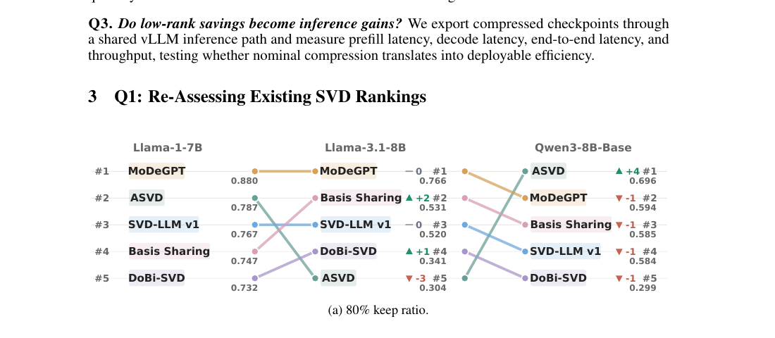
The core evidence for the paper’s headline claim is Table 1 and Figure 4, and the pattern is genuinely striking once you see it laid out: at an 80% keep ratio, MoDeGPT is the clear #1 on both Llama-1-7B (0.880 MCQ avg) and Llama-3.1-8B (0.766), but on Qwen3-8B-Base it drops to #2 (0.594), overtaken by ASVD (0.696) — the very method that ranked last (#5, 0.304) on Llama-3.1-8B at the same keep ratio. Basis Sharing shows the opposite pattern: it climbs from #4 on Llama-1-7B to #2 on Llama-3.1-8B, and then drops back to #3 on Qwen3.

Why this happens, mechanically: the paper attributes this to different architectural properties across model families interacting differently with each method’s assumptions. ASVD’s activation-aware rescaling assumes a particular relationship between activation magnitude and singular-value importance that appears to hold well for Qwen3’s activation statistics but poorly for Llama-3.1’s; MoDeGPT’s modular decomposition strategy, which performs adaptive per-module rank allocation, appears to transfer well across the two LLaMA generations (which share substantial architectural lineage) but not as well to Qwen3’s differently-structured attention/MLP blocks. The paper is careful to note this is an empirical observation, not a fully explained causal mechanism — no single method’s design is shown to definitively fail for a specific, identified architectural reason; the paper’s contribution is demonstrating that the instability exists and is large, not explaining its root cause layer-by-layer.

The 60% keep ratio panel (not reproduced here in full, see the paper’s Table 1) shows the same qualitative pattern: MoDeGPT and Basis Sharing swap the top two spots between Llama-1-7B and Llama-3.1-8B, while Basis Sharing becomes the outright leader on Qwen3-8B-Base at this more aggressive budget.

Design-choice discussion — why three backbones, and is that enough? Testing across architecturally distinct model families (legacy LLaMA vs. modern Llama-3.1 vs. Qwen3) is the right minimal experiment to demonstrate non-invariance — a single backbone could never show this effect at all. The obvious alternative — testing many more backbones (Mistral, Gemma, DeepSeek, etc.) — would strengthen the generality claim further, and its absence is a genuine scope limitation: with only three backbones (two of which share the LLaMA lineage), we cannot yet say whether “architecture-dependent ranking instability” is a universal property of SVD compression or specific to whatever differs between LLaMA-style and Qwen-style transformer blocks (RMSNorm placement, QK-normalization, GQA head-group configuration, etc. — several of these architectural details plausibly interact with which weight directions carry the most “important” activation-aligned signal).

Perplexity reveals a gap that accuracy metrics hide

The paper’s second major finding, and arguably the more actionable one for practitioners, is visible directly in Table 1’s PPL columns: at the 60% keep ratio on Llama-3.1-8B, SVD-LLM and Basis Sharing reach C4 perplexities of 1187.78 and 461.21 respectively — compare this to the dense model’s C4 PPL of 9.10. These are not “somewhat worse,” they are qualitatively broken: a perplexity in the hundreds or thousands typically corresponds to a model producing largely incoherent text. Yet these same two methods’ MCQ averages (0.425 and 0.469 respectively — see full Table 1) remain well above the 35.7% random-choice floor the paper computes for its seven-task MCQ suite.

Why this discrepancy matters and isn’t just a curiosity. MCQ tasks only require the model to assign a higher log-probability to the correct answer choice than to the (typically 2–5) alternatives — a coarse relative-ranking signal that survives even fairly severe degradation of the model’s overall generative distribution. Perplexity, by contrast, requires the model’s predicted distribution over the entire vocabulary to stay close to the true distribution at every token position in fluent, open-ended text. A model can retain “which is more plausible, A or B” judgment while completely losing the ability to produce coherent free-form text — precisely the gap this paper’s dual-metric protocol is designed to expose. If a compression-method paper reports only MCQ accuracy (a common practice the paper’s Fig. 2 audit implicitly critiques), it can hide a compression regime that would be unusable for any open-ended generation task (chat, code, summarization) while still looking respectable on a leaderboard.

The paper is careful to add a nuance here too: ASVD’s 0.353 MCQ average at 80% keep on Llama-3.1-8B sits almost exactly at the 0.357 random-choice floor — meaning this particular number should be read as “no retained capability” rather than “modest degradation,” a distinction that a bare percentage number alone would not convey without the floor being explicitly computed and reported.

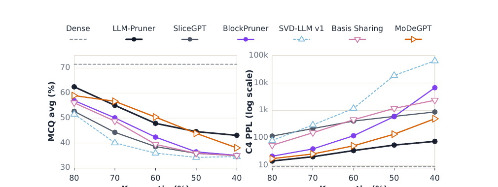
Q2: SVD vs. structured pruning — competitive on accuracy, behind on generative stability

Comparing against LLM-Pruner, SliceGPT, and BlockPruner under matched parameter budgets (Figure 3 above, left panel), SVD methods remain broadly competitive on MCQ accuracy across the full 80%→40% keep-ratio range — no dramatic gap opens up there. But the right panel (C4 perplexity, log scale) tells a different story: at the 60% keep ratio, MoDeGPT’s PPL of 51.82 (the best among the tested SVD methods) still trails LLM-Pruner’s 34.85, and several other SVD methods are one to two orders of magnitude worse. The paper’s summary judgment: SVD is competitive with pruning on the coarse accuracy metric, but exhibits a “capability cliff” in generative fluency under aggressive compression that pruning avoids more gracefully — likely because pruning removes entire structural units (leaving surviving components as intact, unmodified sub-networks) whereas SVD reconstructs every remaining weight as an approximation, so approximation error compounds across every single retained parameter rather than being concentrated at removal boundaries.

Design/experimental-choice caveat the paper itself raises: this Q2 comparison explicitly excludes any post-compression recovery fine-tuning for both pruning and SVD methods (matching the “no added recovery” policy from the Algorithm 1 pseudocode above), and the paper is careful to state that this ranking might not hold once each method’s default recovery protocol is reintroduced — an honest scope-limiting statement that prevents overclaiming from this specific experiment.

Q3: The FLOP-savings-to-latency gap

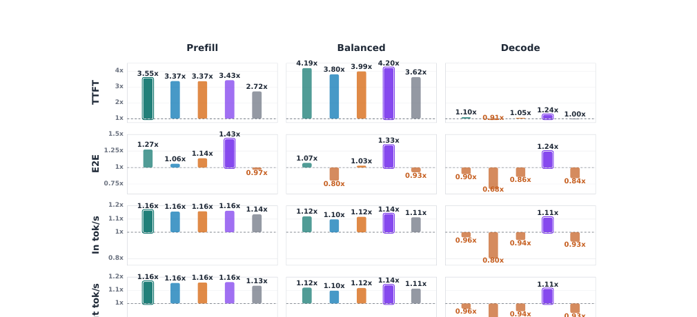
This is, in my assessment, the paper’s single most practically important finding, because it directly contradicts an assumption implicit in almost every SVD compression paper’s abstract: that “N% fewer parameters/FLOPs” translates into “N%-ish faster inference.” The measured reality, using a matched vLLM serving harness across the same hardware, precision, and request stream for every method:

• Prefill-heavy profile (long input, short output): TTFT speedups of 2.72x–4.20x across the five methods — this is the regime where reduced FLOPs genuinely helps, because prefill is compute-bound.
• Decode-heavy profile (short input, long output): end-to-end throughput speedups collapse to a range of 0.68x–0.91x — meaning every tested method, including the best, is slower than the uncompressed dense baseline once decoding dominates the workload.

Why this happens, mechanically, tying back to the Prerequisites section: decode-time inference issues one token’s worth of computation per step, which turns every matrix multiply into a “thin” GEMM (small batch/sequence dimension against a large weight matrix). In this regime, the bottleneck is streaming the weight matrix from HBM into the GPU’s compute units, not doing the arithmetic — so replacing one large, well-optimized dense GEMM kernel with two smaller low-rank GEMM kernels (the $A(Bx)$ decomposition from the SVD section) adds kernel-launch overhead and intermediate-tensor memory traffic without proportionally reducing the memory-bandwidth bottleneck that’s actually gating performance. Two cheap-in-FLOPs kernels executed sequentially can lose to one expensive-in-FLOPs kernel executed once, precisely because FLOPs were never the bottleneck to begin with in this regime.

A necessary caveat the paper itself flags: DoBi-SVD implements a dense fallback — for layers where the retained rank is high enough that the low-rank factorization wouldn’t actually save memory bandwidth, it falls back to executing the layer as one dense GEMM instead of two low-rank GEMMs. This means DoBi-SVD’s measured speedup numbers are not purely attributable to “low-rank factorization is fast”; they partly reflect a hybrid runtime policy decision about when not to use low-rank execution at all. The paper is explicit about this, which is a good sign for interpretability, but it also means the Figure 4 (paper’s Fig. 6) comparison is not perfectly apples-to-apples across all five methods — some of what’s being measured is algorithm quality, and some is runtime engineering sophistication.

The secondary audits: calibration sensitivity, larger models, more devices

Beyond the three headline questions, the paper runs several smaller, more targeted audits that are worth summarizing because they each probe a different potential objection to the main results:

• Calibration sensitivity (Table 2): on Llama-3.1-8B at 80% keep, varying only the calibration corpus (WikiText-2 vs. C4 vs. Pile-Val) while holding everything else fixed shows the ranking order stays stable across three WikiText-2 resamples, but the exact scores shift, and the close Basis Sharing–SVD-LLM pair actually flips when calibrated on C4 instead of WikiText-2. This means the un-standardized “native calibration recipe per method” compromise from Algorithm 1’s Step B does introduce some genuine uncertainty into close rankings, though not enough to overturn the “clear leader” cases (margins there are larger than the observed calibration-induced variance).
• 70B feasibility audit: attempting to scale each method to a 70B-parameter model on a single H200 GPU under a fixed compute budget, the paper finds every single tested method hits an engineering wall before an algorithmic one: ASVD is blocked by a legacy lm_eval dependency conflict, SVD-LLM v1 and DoBi-SVD hit GPU memory ceilings, Basis Sharing crashes in its CUDA eigensolver step, and MoDeGPT fails during Accelerate’s GPU-offloading logic. None of these are fundamental algorithmic limits — they’re software maturity gaps — but the paper is right to flag this as a real “implementation readiness” dimension that’s invisible if you only look at reported 7B-scale numbers.
• Cross-device robustness (Table 3): rerunning SVD-LLM v1 at a 60% keep ratio on an RTX A5000 (rather than the primary A100) shows the same qualitative pattern as the main result — large TTFT gains (3.37x–3.80x) that shrink or invert (0.68x–1.06x) at the end-to-end level depending on workload phase — suggesting the prefill/decode asymmetry finding is not an A100-specific artifact.

Quantitative Results, Reproduced in Full: Llama-3.1-8B

To make the ranking-instability claim concrete rather than just described in prose, it’s worth reproducing the paper’s actual Llama-3.1-8B numbers at the 80% keep ratio (Table 1 in the original), since this is the backbone where the ranking most dramatically diverges from the legacy Llama-1-7B numbers discussed above.

Method	WikiText-2 PPL ↓	C4 PPL ↓	BoolQ	ARC-E	ARC-C	WinoG.	PIQA	HellaS.	OBQA	MCQ Avg ↑	MathQA	MMLU-Math
Dense FP	6.24	9.10	0.831	0.824	0.549	0.746	0.812	0.793	0.454	0.716	0.396	0.437
ASVD	2011.38	1281.96	0.382	0.285	0.226	0.512	0.536	0.285	0.244	0.353	0.201	0.223
SVD-LLM v1	14.83	80.94	0.661	0.528	0.315	0.645	0.639	0.476	0.350	0.516	0.256	0.305
DoBi-SVD	556.59	1008.41	0.378	0.298	0.226	0.516	0.522	0.282	0.266	0.355	0.205	0.292
Basis Sharing	15.61	54.36	0.632	0.637	0.367	0.667	0.701	0.548	0.372	0.561	0.248	0.297
MoDeGPT	9.01	17.68	0.412	0.715	0.436	0.730	0.743	0.710	0.382	0.590	0.344	0.407

A few things become visible only once these numbers are laid out in full rather than summarized:

• MoDeGPT’s aggregate lead (0.590 MCQ Avg) partially masks a weak BoolQ score (0.412) that would look like a red flag in isolation — it wins primarily on ARC-E/ARC-C/WinoGrande/PIQA/HellaSwag, not uniformly across all seven tasks. Basis Sharing, despite a lower aggregate (0.561), actually beats MoDeGPT on raw BoolQ (0.632 vs. 0.412). This is the concrete evidence behind the paper’s claim that aggregate rankings reflect “a trade-off between generative stability and downstream accuracy, rather than a universal ordering of method quality” — no single method dominates on every task simultaneously, even within one backbone at one keep ratio.
• The PPL columns swing far more violently than the MCQ columns across methods. DoBi-SVD’s C4 PPL (1008.41) is roughly 111x the dense baseline’s 9.10, while its MCQ Avg (0.355) is only about 50% below the dense baseline’s 0.716 — a striking numerical illustration of the earlier “perplexity is far more punishing than MCQ accuracy” argument, visible directly in this single row of real data rather than as an abstract claim.
• SVD-LLM v1 and Basis Sharing’s PPL values (80.94 and 54.36) are both far worse than MoDeGPT’s (17.68) despite having reasonably competitive MCQ averages (0.516 and 0.561 vs. 0.590) — a roughly 5x worse C4 perplexity for a method that trails by only 5–13 percentage points on MCQ Avg is exactly the kind of PPL/MCQ divergence this paper’s dual-metric protocol is designed to surface, and it would be invisible to anyone reading only an MCQ-based leaderboard.

Critical Analysis

(a) Weaknesses and flaws specific to this paper.

• The methods audited are all from 2023–2025; the field has kept moving. The five re-evaluated methods (ASVD 2023; SVD-LLM, Basis Sharing, MoDeGPT 2024; DoBi-SVD 2025) do not include several 2026 methods this very blog series has already covered — SigmaScale, AIR, Swift-SVD, LACE-SVD, SVD-Surgeon, GRASP, Zero-Sum SVD, or CARE-LoRA. The paper’s related-work section acknowledges most of these exist (citing several by reference number) but does not re-run them through the standardized harness. This means the paper’s specific numerical rankings are already somewhat dated relative to the field’s current frontier at the time of publication, even though its methodological point — rankings are context-dependent, standardize before trusting a leaderboard — remains valid and arguably applies with equal force to the newer methods it didn’t test.
• Only five methods is a narrow sample for a paper whose whole point is “rankings aren’t stable.” Demonstrating instability across five methods and three backbones is suggestive but not dispositive; a larger sample (say, 10–12 methods) would make the “no stable ranking exists” claim considerably more convincing, since with only five candidates, rank permutations are combinatorially limited (5! = 120 possible orderings), and observing “the ranking changed” across three backbones is a comparatively easy bar to clear even under substantial measurement noise alone.
• The paper doesn’t report confidence intervals or repeated runs for the main Table 1 leaderboard. The calibration-sensitivity audit (Table 2) does report a standard deviation for WikiText-2 resamples on one backbone at one keep ratio, but the primary leaderboard numbers in Table 1 — the ones the ranking-shift claims (Figure 4/Q1) are built on — are apparently single point estimates. Without knowing the run-to-run variance of, say, MCQ average under a fixed calibration set but different random seeds elsewhere in the pipeline (e.g., evaluation harness shuffling, tie-breaking in argmax scoring), it’s hard to fully distinguish “genuine architecture-dependent ranking instability” from “measurement noise that happens to be somewhat larger than typically assumed.” The Table 2 audit partially mitigates this concern (showing the largest within-WikiText-2 range, 0.0284, is smaller than most reported leader margins) but doesn’t cover every cell of the main table.

(b) Limitations the authors understate or omit.

• The paper doesn’t report which layers/modules each method chose to compress more or less aggressively, despite this being the most likely mechanistic explanation for the architecture-dependent ranking shifts. Given that the keep-ratio formula (derived above) is a parameter-weighted aggregate that hides per-layer allocation choices, understanding why MoDeGPT transfers well across LLaMA generations but not to Qwen3 would require exactly this per-layer breakdown, which the paper does not provide even in the appendix sections summarized. This is a missed opportunity to turn an empirical observation (“rankings shift”) into a mechanistic explanation (“rankings shift because method X allocates rank to attention projections while method Y allocates it to MLP projections, and Qwen3’s GQA configuration changes which allocation strategy is favorable”).
• The BoolQ anomaly (a 0.41 score for one method, flagged as “exactly reproduced… reflects a strong output-label bias”) is mentioned but not deeply investigated in the main text. The paper defers this to an appendix (“Appendix B.6”), but a reproducible, deterministic anomaly in a widely-used benchmark task is exactly the kind of finding that could matter beyond this one paper’s scope — if a specific compressed model configuration systematically biases toward one label on BoolQ regardless of the actual question, that’s evidence about calibration/compression interaction that other MCQ-heavy compression papers should probably be checking for too, and a fuller treatment in the main paper (rather than an appendix pointer) would have strengthened the contribution.
• The “no consistent advantage over structured pruning” framing in the abstract slightly overstates what Q2’s evidence supports. The MCQ-competitive, PPL-behind pattern found is a real and important nuance, but “no consistent advantage” reads as a stronger claim than the underlying evidence (one backbone, no recovery fine-tuning applied to either family) can fully support — the paper’s own text is more careful about this nuance than its abstract-level summary phrasing.

(c) Concrete, specific improvement suggestions.

1. Extend the standardized harness to at least 10 methods spanning 2023–2026, including the newer activation- and loss-aware variants this blog has covered (SigmaScale, AIR, Swift-SVD, GRASP, Zero-Sum SVD), to test whether the “no stable ranking” finding strengthens, weakens, or reveals a different pattern (e.g., perhaps newer methods do converge to a more stable ranking as the field matures, which would itself be an interesting and testable hypothesis).
2. Report per-layer rank allocation profiles for each method on each backbone, at least as a supplementary visualization (e.g., a heatmap of retained rank fraction by layer index and layer type, attention vs. MLP), to turn the “architecture-dependent instability” observation into an actionable mechanistic hypothesis that future method designers could test against.
3. Run the main Table 1 leaderboard with at least 3 random seeds per cell (varying whatever stochastic elements exist in the harness, even holding the calibration corpus fixed) and report standard errors alongside point estimates, so readers can distinguish “this specific ranking shift is a robust finding” from “this specific ranking shift is within the noise floor of the measurement pipeline” — a distinction the paper’s own careful, evidence-driven style suggests the authors would want to get right if resources permitted.

Extended Note: Why the Aggregate/Per-Task Gap Also Matters for Deployment Decisions

One implication worth spelling out explicitly, because it’s easy to read past a results table without internalizing it: if you are choosing an SVD compression method for a specific production use case rather than for a paper’s leaderboard, the aggregate MCQ average in Table 1 is close to the least useful number in the whole paper for your decision. Suppose your production system is a factual-QA assistant that leans heavily on yes/no and true/false style judgments (BoolQ-like) rather than commonsense completion (HellaSwag-like) or physical-reasoning (PIQA-like) judgments. Looking only at the aggregate MCQ average, MoDeGPT (0.590) would appear to dominate Basis Sharing (0.561) on Llama-3.1-8B at 80% keep. But looking at the BoolQ-specific column, Basis Sharing (0.632) clearly outperforms MoDeGPT (0.412) — a reversal that the aggregate number actively hides. This is not a hypothetical concern manufactured for this review; it follows directly from the per-task breakdown reproduced above, and it is exactly the kind of task-composition sensitivity that a practitioner evaluating these methods for a specific downstream application should check directly against their own task mix rather than trusting any single aggregate leaderboard number — the paper’s own methodological lesson (standardize before trusting a comparison) applies recursively to how a reader should treat this paper’s own aggregate columns.

Feasibility and Cost: The Hidden Fourth Axis

One finding that deserves more attention than a single paragraph, because it’s the least “algorithmic” and most “engineering-practical” result in the paper: the 70B feasibility audit is arguably a preview of what practitioners will actually hit first when trying to adopt any of these methods at real production model scale, well before they get to argue about whether the accuracy numbers are competitive.

Why this matters mechanically. SVD compression’s computational bottleneck during the compression step itself (not inference — the one-time cost of producing the compressed checkpoint) is typically the singular value decomposition computation on large matrices, plus, for activation-aware methods like ASVD and SVD-LLM, a calibration forward pass to collect activation statistics that must fit in memory alongside the model itself. At 7–8B scale, this fits comfortably in a single high-memory GPU. At 70B scale, the calibration forward pass alone requires either a multi-GPU tensor-parallel setup or CPU/disk offloading — and it is precisely at this transition point that the paper found every tested method’s released implementation (not the underlying algorithm) breaks in a distinct way:

Method	Failure mode at 70B (single H200)	Root cause category
ASVD	Blocked by legacy lm_eval dependency	Software dependency staleness
SVD-LLM v1	Hits memory ceiling	No offloading support in released code
DoBi-SVD	Hits memory ceiling	No offloading support in released code
Basis Sharing	Crashes in CUDA eigensolver	Numerical kernel not validated at this matrix scale
MoDeGPT	Fails during Accelerate GPU-offloading	Offloading integration incompatibility

Design-choice discussion — why frame this as “implementation readiness” rather than “algorithmic scalability,” and where that framing could still mislead. The paper is careful to separate these two questions, and the distinction is analytically important: none of these five failure modes is a proof that the underlying mathematical approach (SVD-based factorization, activation-aware rescaling, adaptive rank allocation) cannot scale to 70B — in each case, a sufficiently motivated engineering team could very likely patch the specific dependency, add offloading support, or swap the eigensolver. The boundary case worth flagging, though: this framing could be read as reassuring practitioners that the accuracy/ranking findings (Q1/Q2) will hold once engineering catches up — but the paper never actually demonstrates this, since none of the five methods was successfully run to completion at 70B under the fixed one-H200 budget. It remains an open, untested question whether MoDeGPT’s Llama-family advantage or Basis Sharing’s stronger tail-task performance would persist, strengthen, or reverse at 70B scale; readers should not extrapolate the 7–8B ranking findings to larger models without independent verification, a caveat the paper’s abstract does not foreground as prominently as its Q1 ranking-instability finding.

Reproducibility Notes

• Code and checkpoint zoo: the paper states the full platform, standardized method adapters, and over 3 TiB of compressed checkpoints are released at https://github.com/Zishan-Shao/lowrankarena.git, with checkpoints separately hosted at https://huggingface.co/Duke-CEI-SVD/LowRankArena. Releasing the actual compressed checkpoints (not just code) is a meaningfully stronger reproducibility commitment than most compression papers make, since it lets a third party skip the (often GPU-expensive) compression step entirely and go straight to independent re-evaluation.
• Task/harness versions: LM-Eval-Harness v0.4.11, vLLM 0.18.1 — both explicitly version-pinned, which matters because both libraries have historically changed default scoring behaviors and serving performance characteristics across versions in ways that would silently break exact reproducibility if left unpinned.
• Hardware: primary results on one NVIDIA A100 80GB PCIe GPU; cross-device robustness checks additionally use RTX A5000, L40S, and a single H200 141GB for the 70B feasibility audit — a genuinely accessible hardware bar for the 7–8B-scale primary experiments, though the 70B feasibility work requires H200-class access most independent researchers won’t have.
• What’s not fully specified in the excerpted main text: the exact request-arrival process parameters, warmup counts, and percentile-reporting conventions are stated to live in the appendix tables (A.1/A.2), which is standard practice, but means a reader relying only on the main body (as most citations of this paper likely will) would need to consult the appendix or released YAML configs to exactly reproduce the inference-benchmark numbers in Figure 4 (paper’s Fig. 6).

Full 60% Keep-Ratio Table for Comparison

To round out the quantitative picture beyond the 80% keep-ratio table reproduced above, here is the 60% keep-ratio row on Llama-3.1-8B — the more aggressive compression regime where the paper’s “capability cliff” finding is most visible:

Method	WikiText-2 PPL ↓	C4 PPL ↓	BoolQ	ARC-E	ARC-C	WinoG.	PIQA	HellaS.	OBQA	MCQ Avg ↑	MathQA	MMLU-Math
ASVD	22684.63	14186.23	0.405	0.254	0.257	0.491	0.507	0.260	0.284	0.351	0.192	0.286
SVD-LLM v1	199.84	1187.78	0.378	0.295	0.246	0.533	0.515	0.283	0.268	0.360	0.205	0.257
DoBi-SVD	987.51	1529.38	0.378	0.271	0.251	0.481	0.511	0.265	0.288	0.349	0.203	0.268
Basis Sharing	82.96	461.21	0.380	0.409	0.241	0.562	0.568	0.325	0.284	0.396	0.205	0.211
MoDeGPT	24.50	51.82	0.622	0.460	0.312	0.672	0.629	0.516	0.316	0.504	0.241	0.213

Comparing this to the 80% keep-ratio table above makes the “capability cliff” language concrete: ASVD’s C4 PPL jumps from 1281.96 (80% keep) to 14186.23 (60% keep) — an 11x further degradation from a comparatively modest 20-percentage-point reduction in keep ratio, while MoDeGPT’s C4 PPL only roughly triples (17.68 → 51.82) over the same budget reduction. This asymmetric sensitivity to the keep-ratio axis is itself method-dependent, and is not visible at all if you only ever look at one keep ratio in isolation — a further argument for why the paper’s multi-ratio sweep design (rather than a single-point comparison) was necessary to expose the instability finding.

What This Means for the Rest of This Blog Series

Since this series has already reviewed several individual SVD compression papers as if each one represented incremental progress, it’s worth being explicit about how this paper should retroactively recalibrate how those reviews are read. This is not a retraction of any individual method’s contribution — SigmaScale’s learned scaling matrices, AIR’s activation-and-influence-aware weighting, Swift-SVD’s optimality guarantees, and GRASP’s adaptive singular parameters are each legitimate, well-motivated technical ideas, evaluated honestly within the scope their authors chose. What LowRankArena changes is the confidence with which any single paper’s own reported comparison table should be read as a durable, cross-context ranking rather than a snapshot valid under one specific backbone, budget, and metric combination. Going forward, this series will treat any individual SVD compression paper’s “we beat prior SOTA” claim as a claim about that paper’s specific evaluation conditions first, and only secondarily as evidence about general superiority — exactly the discipline LowRankArena’s own methodology recommends.

A Second Worked Example: Interpreting the Inference-Speedup Numbers Precisely

It’s worth pushing one more concrete calculation through the paper’s actual reported numbers, because “4.20x TTFT speedup, 0.80x E2E throughput” is easy to state but easy to misread without doing the arithmetic. Table 3 (the cross-device audit on RTX A5000) gives raw millisecond numbers alongside the speedup ratios for SVD-LLM v1 at a 0.6 keep ratio:

• Prefill-heavy profile: TTFT drops from 3417ms (dense) to 1013ms (compressed) — a genuine 3.37x reduction in time-to-first-token, meaning a user waits roughly one-third as long to see the first generated token. But E2E latency only drops from 4925ms to 4659ms, a mere 1.06x — because the prefill-heavy profile still generates 32 output tokens (see the profile table in the Prerequisites section above), and that decode tail, unaffected by the compression’s prefill-side benefit, dominates the total wall-clock time once you look at the full request rather than just the first token.
• Balanced profile: TTFT improves 3.80x (1668ms → 439ms), but E2E latency actually gets worse: 5905ms → 7358ms, a 0.80x “speedup” (i.e., a genuine slowdown). This happens because the balanced profile’s 128 output tokens amplify the decode-time cost identified earlier (two low-rank GEMMs per step instead of one dense GEMM), and this per-token decode overhead, multiplied across 128 steps, more than cancels out the prefill-time savings.
• Decode-heavy profile: TTFT barely changes (187ms → 205ms, actually a 0.91x “speedup” i.e. slightly slower, since there’s almost no prefill work to save time on), and E2E latency degrades substantially: 15136ms → 22359ms, a 0.68x ratio — nearly 50% slower wall-clock time for the full request when the workload is decode-dominated.

Why walking through this matters beyond the paper’s own summary chart: the raw millisecond numbers make visible something the ratio-only presentation (Figure 6 in the main results) can obscure — the absolute latency increase in the decode-heavy case (7,223ms added) is larger in raw terms than the absolute latency saved in the prefill-heavy case (2,404ms + 266ms saved across TTFT and residual). If a real production system’s request mix is even modestly decode-heavy (which most conversational and agentic LLM workloads are, since output length typically exceeds input processing marginal cost per request), the net effect of deploying this specific compressed checkpoint could be a worse average user-facing latency than the dense model, even though every individual TTFT number in isolation looks like an improvement. This is precisely the trap the paper’s Q3 finding is designed to prevent readers from falling into, and it’s only fully visible once you look at absolute latencies rather than ratios alone.

One More Design Choice Worth Naming: Why Five Methods and Not Fewer or More

A question a careful reader should ask of any benchmark paper: was the sample size (five methods) chosen for a principled reason, or was it simply “whatever was reproducible in the time available”? The paper’s own framing (“publicly reproducible SVD-style methods”) suggests the latter is closer to the truth — ASVD, SVD-LLM, DoBi-SVD, Basis Sharing, and MoDeGPT were selected specifically because their original implementations were available and could be adapted to the shared harness, not because they were pre-selected as maximally representative of the method-design space (e.g., there’s no method here representing purely learned/differentiable rank allocation as a primary mechanism, distinct from MoDeGPT’s modular decomposition). This is a defensible and honest way to build a first version of a standardization platform — you audit what you can actually get running — but it does mean the five-method sample is a convenience sample with respect to reproducibility, not a stratified sample with respect to algorithmic design space. The paper is transparent that DoBi-SVD’s repeated compression runs did not complete within its available compute budget for the calibration-sensitivity audit (Table 2), which is itself a small piece of evidence for this point — reproducibility constraints shaped which comparisons could even be attempted, not just which methods were included in the first place. A natural, testable prediction from this observation: the next iteration of a platform like this should report a principled taxonomy of the SVD-compression design space (activation-aware vs. loss-aware truncation; per-layer vs. cross-layer allocation; static vs. learned rank selection) and select at least one representative from each cell, rather than defaulting to whichever five methods happen to have maintained, working public repositories at the time of writing.

A Note on Terminology: “Standardization” vs. “Benchmarking”

It’s worth being precise about what kind of contribution this actually is, because the terms “benchmark paper” and “standardization platform” get used loosely and interchangeably in ML systems venues, but they imply different epistemic commitments. A pure benchmark paper’s job is to answer “which method wins on task X” — it optimizes for a clean, decisive leaderboard. A standardization paper’s job, which is closer to what LowRankArena actually does, is to answer “can we even trust that the leaderboard means what it claims to mean” — its success criterion is not a decisive winner, but a defensible, reproducible measurement protocol that other researchers can build on, even if (as happened here) the headline finding is uncomfortable for the field it audits. Judged by this standard — not “did it crown a winner” but “did it produce a protocol others can trust and extend” — LowRankArena succeeds precisely because its main empirical result (no stable ranking) would have been impossible to state credibly without the standardization machinery described in this review’s earlier sections. A benchmark paper chasing a decisive winner would have had an incentive to suppress or downplay exactly this kind of instability finding; a standardization paper’s incentives point the opposite way, toward surfacing it.

A Closing Methodological Note on Generalizing Beyond SVD Compression

One last point worth making explicit before the conclusion: the standardization discipline this paper demonstrates — fix the budget definition, fix the task suite, fix the inference harness, separate the algorithmic axis from auxiliary axes, then re-measure everyone under the same conditions — is not specific to SVD compression at all. The exact same recipe could, and arguably should, be applied to quantization methods (where “4-bit” means different things depending on group size and outlier handling), to speculative decoding methods (where “acceptance rate” depends heavily on the specific draft/target model pairing and decoding temperature), or to KV-cache compression methods (where “compression ratio” claims often bundle eviction policy changes with quantization in ways analogous to the SVD/mixed-precision conflation this paper isolates). Readers of this blog series who have followed the quantization, speculative-decoding, and KV-cache-compression review threads should read this paper’s methodology as a template rather than a one-off audit — the same protocol-fragmentation problem this paper diagnoses for SVD compression very plausibly exists, largely unaudited, in each of those adjacent subfields too.

Conclusion

LowRankArena’s contribution is not a new compression trick — it’s a mirror held up to an entire subfield, and what it shows is not flattering to the “monotonic progress” narrative that individual papers (including several I’ve reviewed in this series) tend to imply. The core finding — that SVD-compression method rankings are architecture-, budget-, and metric-dependent rather than universal — is exactly the kind of result that’s uncomfortable to publish (it doesn’t advance anyone’s specific method) but valuable to have in the literature, because it changes how the next reader of any single SVD compression paper’s results table should calibrate their confidence in a reported “beats prior SOTA” claim.

The most actionable single takeaway for practitioners, in my view, is the third finding: don’t trust “N% FLOP reduction” as a proxy for “N%-ish faster inference” without measuring end-to-end decode-heavy throughput specifically, because the prefill/decode asymmetry this paper documents (up to 4.2x prefill speedup collapsing to sub-1x decode throughput) means the workload you actually care about — which, for most production chat/agent/code-generation use cases, is decode-dominated — is exactly the regime where nominal low-rank savings are least likely to show up as real wall-clock benefit. If you’re evaluating an SVD compression method for deployment rather than for a paper’s leaderboard, this paper’s methodology (not just its five-method snapshot) is the more durable thing to take away: insist on a matched, end-to-end, decode-heavy inference benchmark before trusting any reported speedup number, in the same spirit this paper insists on a matched, standardized accuracy benchmark before trusting any reported “new SOTA” claim.

Finally, for readers who track this blog series week to week: expect the next several SVD/low-rank compression reviews to explicitly cite this paper’s protocol whenever they discuss a claimed accuracy or speed improvement, and expect this reviewer to hold future “beats prior SOTA” claims to the standard LowRankArena sets — matched backbone, matched keep-ratio definition, matched precision, and a decode-heavy end-to-end inference number, not just a headline ratio. That is the single most durable habit a reader of this literature can adopt from this paper, and it costs nothing but a moment’s skepticism before accepting any single results table at face value.

Quick-Reference Checklist for Evaluating Any Future SVD Compression Claim

As a practical closing summary, distilled from every design choice discussed above, here is a concrete checklist to apply the next time a new SVD-based LLM compression paper crosses your desk — whether in this blog series or elsewhere:

1. Is the keep-ratio/compression-ratio definition stated precisely enough to compute independently? Check for the precision-matching clause specifically (Section 2.2’s formula above) — if a paper doesn’t state whether its reported ratio holds precision fixed, assume it might not, and discount the number accordingly.
2. Is perplexity reported alongside multiple-choice accuracy, on a held-out corpus separate from any calibration set? A paper reporting only MCQ accuracy for a generative compression method should raise a flag, per the PPL/MCQ divergence evidence reproduced in this review’s Table 1 excerpt.
3. Is the comparison to structured pruning present, and at a matched parameter budget? If a paper only compares against other SVD methods, ask whether it would still look favorable against a pruning baseline at the same budget — this paper’s Q2 finding suggests the answer is often “less favorable than it appears.”
4. Is there an end-to-end, decode-heavy inference measurement, not just a FLOP or parameter-count reduction? Per the Q3 finding and the worked TTFT/E2E example above, a compression method with impressive prefill speedups can be a net slowdown for decode-dominated production workloads — always ask for the decode-heavy number specifically.
5. Is the result validated on more than one model family? Given the architecture-dependent ranking instability demonstrated in Figure 2/4 above, a result shown only on a single backbone (especially only on legacy LLaMA-1/2) should be treated as preliminary rather than general.
6. Are calibration set size and composition disclosed, and is there any sensitivity analysis? Per Table 2’s finding that close rankings can flip under a different calibration corpus, an undisclosed or unvaried calibration recipe is a real, if secondary, source of uncertainty in any reported ranking.

Applying even three or four of these six checks to any new paper in this space will typically surface most of the comparability issues this review has walked through in detail — which is, in the end, exactly the point LowRankArena itself is trying to make.

Appendix Notes: Terminology Cross-Reference

For readers newer to this specific corner of the literature, a short glossary cross-referencing terms used throughout this review to their first-appearance context, since several are used precisely and interchangeably with the paper’s own notation:

• Keep ratio ($r$): the fraction of original parameter count retained after compression, formally defined in the “Standardized Keep-Ratio Formula, Expanded” section above; equivalently, $1-r$ is the fractional parameter reduction.
• Rank fraction: $k/\min(m,n)$ for a single layer — a different, more granular quantity than the aggregate keep ratio $r$; the worked numerical example above shows these two can diverge substantially for the same compressed model.
• TTFT (time-to-first-token): the latency between a request arriving and the first output token being produced; dominated by prefill compute.
• E2E (end-to-end) latency: the total latency for an entire request, from arrival to the final output token; the sum of prefill time plus the full decode sequence.
• MCQ Avg: the macro-averaged zero-shot accuracy (or normalized accuracy, acc_norm, where available) across the seven multiple-choice tasks listed in the Prerequisites section (BoolQ, ARC-Easy, ARC-Challenge, WinoGrande, PIQA, HellaSwag, OpenBookQA).
• Native calibration recipe: the specific calibration dataset and sample count each method’s original authors specified as their default (e.g., ASVD’s 32 WikiText-2 sequences vs. SVD-LLM’s 256) — preserved as-is in LowRankArena’s Algorithm 1 Step B rather than standardized across methods, a deliberate and disclosed compromise.
• Uniform-precision regime: the primary comparison regime in this paper, where compressed and original weights share the same numerical bit-width, isolating the low-rank effect from quantization effects (see the keep-ratio formula’s precision constraint).