SCOUT: Localizing Latent Training Failures via Strict-Majority Consensus Among Equivalent Replicas

Review date: 2026-08-27 | Author: Zhongzhu Zhou Paper reviewed: SCOUT: Symmetric Consensus Outlier Detection for Failure Localization in LLM Pre-Training Paper authors: Zhuang Wang (Independent Researcher) arXiv: 2608.11034 Venue/Status: arXiv preprint, submitted 11 Aug 2026

Why This Paper Matters

If you have ever run a large distributed training job that hung for twenty minutes while every rank sat idle, with no log telling you which of the 3,072 processes was actually stuck, you already understand the problem this paper is solving. LLM pre-training at scale (thousands to tens of thousands of GPUs) is a synchronous system: every rank in a training step waits on collectives (AllReduce, AllGather, AllToAll, ReduceScatter) before it can proceed. That means a single misbehaving rank — one that hangs, silently runs slow, or silently returns a corrupted numerical value — doesn’t produce a rank-specific symptom. It produces a job-wide symptom: every healthy rank appears to also be “stuck” or “slow,” because they are all waiting on the same barrier.

This is the central diagnostic difficulty SCOUT addresses: synchronization erases the identity of the faulty component. The paper’s contribution is not a new checkpointing system, nor a new communication library — it’s a runtime mechanism that restores that lost identity by comparing “equivalent” ranks (ranks that should be doing the same work) against each other and using majority vote to flag whoever disagrees.

Prerequisites

Before diving into the mechanism, it’s worth grounding a few concepts that the paper assumes readers already have.

Data/model/pipeline/expert parallelism, briefly

Large model training distributes both data and model state across many GPUs (which the paper calls “ranks,” a term borrowed from MPI, meaning one participating process, typically bound to one GPU):

• Data parallelism (DP): Each rank holds a full (or FSDP-sharded) copy of the model and processes a different slice of the training batch. Gradients are averaged across DP ranks via AllReduce (or ReduceScatter+AllGather in ZeRO/FSDP style).
• Tensor parallelism (TP): A single layer’s matrix multiply is split across ranks (e.g., splitting the hidden dimension), requiring AllReduce or AllGather within the layer’s forward/backward pass.
• Pipeline parallelism (PP): Different ranks own different layers (stages) of the network; activations flow forward and gradients flow backward between stages.
• Context parallelism (CP): The sequence dimension is sharded across ranks for very long contexts, requiring specialized attention communication.
• Expert parallelism (EP): In Mixture-of-Experts (MoE) models, different ranks host different experts; tokens are routed to their assigned expert’s rank via an AllToAll collective.
• FSDP (Fully Sharded Data Parallel): Instead of every DP rank holding a full copy of parameters, each rank holds only a shard; before a forward/backward pass touching a given layer, the full parameter is materialized via AllGather, then discarded (freed) afterward, trading extra communication for reduced memory.

A real large-scale job typically combines several of these (“hybrid parallelism”): e.g., a rank might occupy position (data-replica index, FSDP shard index, TP shard, PP stage, CP shard, expert group) simultaneously.

Why synchronous training makes localization hard

Every collective operation is only as fast as its slowest participant. If rank 47 out of 12,288 never enters an AllReduce (because its process crashed, its kernel hung, or it took an exception), then every other rank that did enter the AllReduce blocks until a timeout watchdog fires. Whichever rank happens to be first to notice — and report — the timeout is not necessarily the faulty one; it might just be an innocent bystander sitting at the front of the queue. The paper cites production evidence (from PyTorch’s Flight Recorder analysis) that this is in fact the norm: “almost all observed timeouts arise from desynchronization,” meaning the rank reporting the timeout and the collective visible at that instant are often both victims, not the cause.

Similarly, a straggler (a rank that runs computation slower than its peers, due to hardware degradation, thermal throttling, or a stuck background process) doesn’t show up as “rank 47 is slow” in a naive log — it shows up as “every rank’s iteration time increased,” because all peers wait for rank 47 to finish before the synchronized step can complete.

The worst case is silent data corruption (SDC): a GPU with a defective arithmetic unit or memory cell can compute a wrong but not obviously invalid numerical result — no NaN, no crash, no exception. If this corrupted value is a gradient, and it gets AllReduce’d (summed/averaged) with everyone else’s gradients, the corruption spreads into every rank’s optimizer state within one step, and the identity of the original culprit rank is permanently lost inside the reduced value.

The recovery pipeline this fits into

Resilient LLM pre-training typically has three stages: checkpointing (periodically save a consistent recovery snapshot of model/optimizer state), diagnosis (detect that something’s wrong and localize which resource is responsible), and restart (replace/repair the resource and resume from the last known-good checkpoint). Prior work has strong solutions for checkpointing (e.g., GEMINI’s in-memory, high-frequency checkpoints) and restart mechanics (e.g., TrainMover’s elastic membership changes), but the middle step — diagnosis, specifically localization — is where SCOUT focuses. As the paper notes, citing the Minder paper, manually locating a faulty machine in production can take more than 30 minutes on average, sometimes days.

Core Idea: Latent Failures Are Behavioral Outliers

SCOUT’s foundational insight is deceptively simple, and it’s worth stating precisely because the entire system follows from it:

Localize failures as outliers through strict-majority consensus among equivalent replicas.

“Equivalent replicas” means: in a hybrid-parallel job, many ranks are supposed to be doing exactly the same computation on exactly the same shapes of data (just different data-parallel copies, or different FSDP shards holding the same logical parameter). If you line these ranks up and compare their progress, timing, or numerical output, a healthy majority should agree, and a faulty rank should stand out as the minority.

This converts three different manifestations of “latent failure” into three different kinds of measurable disagreement:

Manifestation	What becomes an outlier
Hang	One rank reports different training-progress coordinates or collective-call metadata than its peers, after the group has stalled.
Straggler	One rank takes measurably longer to complete the same controlled unit of work as its peers.
SDC (silent data corruption)	One rank produces a different deterministic numerical result for the same computation on the same inputs.

The elegance here is that the same consensus machinery (described below as “C3”) handles all three, just with different comparison rules (exact equality vs. robust statistical distance) applied to different kinds of evidence (progress metadata, timing, numerical hashes).

Why this works: three empirical observations

The design is justified by three claims the paper backs with citations to production studies:

1. Failures are rare relative to healthy ranks. An individual fault usually leaves the overwhelming majority of ranks in a job healthy. ByteRobust (a production paper cited here) reports that large-scale training failures normally occur independently on individual nodes, and only 1–2 nodes are typically faulty even in a 9,600-GPU job. This justifies majority vote as a valid discriminator — you’re not trying to distinguish 50/50 splits, you’re trying to find a small minority.
2. Practical hybrid-parallel jobs create natural equivalent-replica groups. Data parallelism (or, absent DP, FSDP sharding) naturally produces sets of ranks executing the same computation graph at the same training step, just on different data or different parameter shards.
3. A rank-local failure breaks behavioral symmetry. The faulty rank will diverge from its equivalent peers in at least one of: collective call order/metadata, elapsed time, or numerical output — even though the failure’s cause (bad transceiver, degraded HBM cell, race condition in a custom kernel) is invisible to the framework.

Design choice: spatial vs. temporal comparison — why/alternative/boundary

A natural alternative to comparing ranks against each other right now (spatial comparison) is to compare a rank against its own history (temporal comparison) — e.g., “rank 47’s forward pass took 40ms last iteration and 400ms this iteration, so it’s a straggler now.”

Why SCOUT chooses spatial over temporal as the primary mechanism: LLM training workloads are highly non-stationary along many axes — different layers have different compute costs, different training steps see different sequence lengths or batch compositions, and MoE routing decisions change which experts (and how much work) each rank handles from step to step. A purely temporal detector would need to model all these legitimate sources of variation and set phase-specific thresholds to avoid false alarms — a much harder modeling problem. Spatial comparison sidesteps this: concurrent peers are, by construction, doing the same work at the same moment, so any difference is attributable to a fault rather than to workload phase.

Where temporal comparison still matters (boundary of spatial-only design): Statistical consensus using the median can, by construction, miss a fleet-wide degradation — if every peer in a group slows down by 10% simultaneously (e.g., due to a shared power or thermal event), no single rank looks like an outlier relative to the others, because the “reference” (the median) has shifted along with everyone else. The paper explicitly acknowledges this: temporal baselines are needed to catch shared/gradual shifts, and SCOUT’s spatial method alone will not catch them. This is a genuine boundary condition, not just a minor caveat — it means SCOUT cannot replace all monitoring, only complement it for the specific class of minority-rank divergence.

Architecture

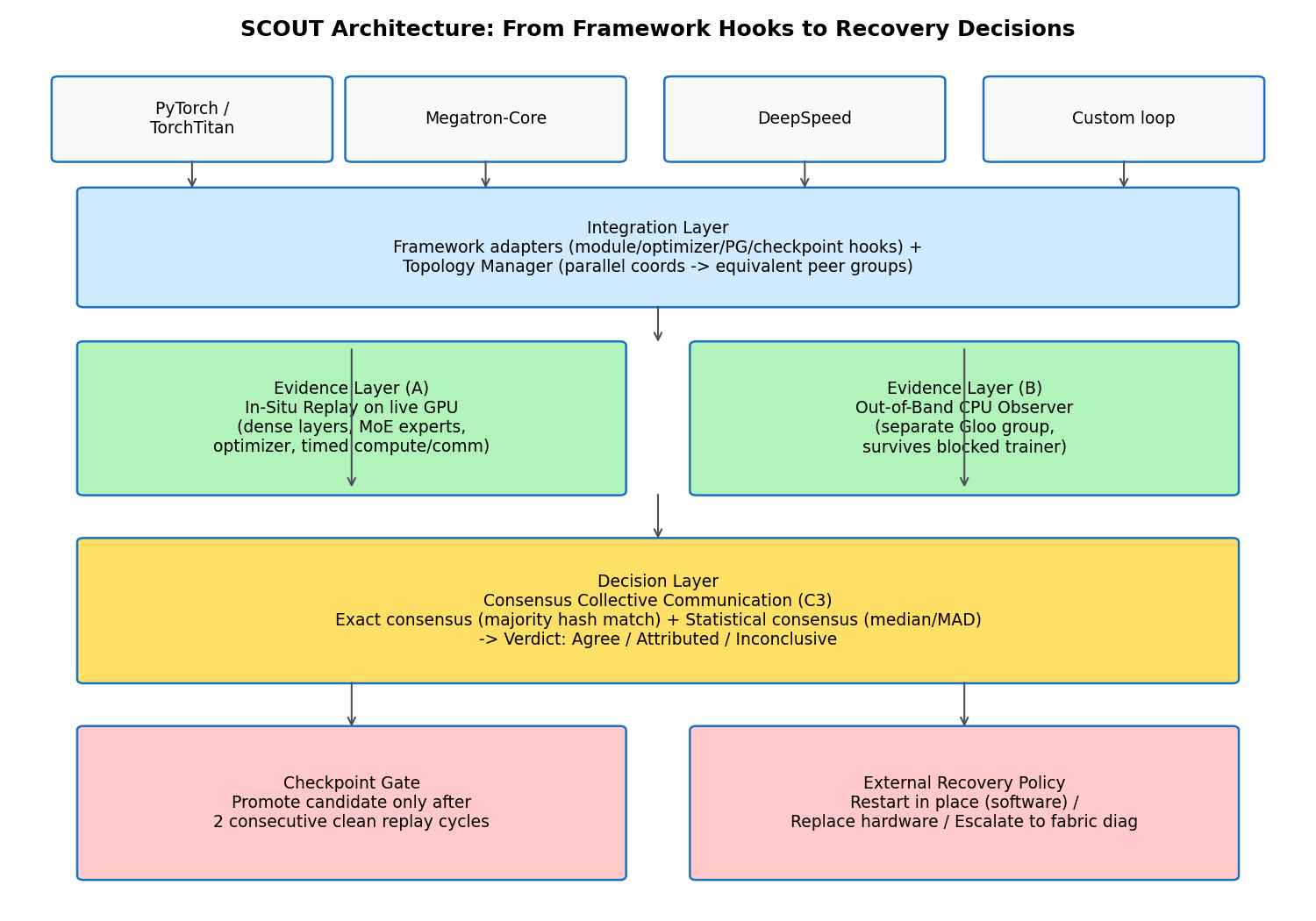
SCOUT’s implementation is organized into three layers, shown conceptually below.

flowchart TB
    subgraph FW["Frameworks"]
        A1[PyTorch] --- A2[TorchTitan] --- A3[Megatron-Core] --- A4[DeepSpeed]
    end
    subgraph INT["Integration Layer"]
        B1["Framework Adapters<br/>(module/optimizer/PG/checkpoint hooks)"]
        B2["Topology Manager<br/>(parallel coords -> equivalent peer groups)"]
    end
    subgraph EV["Evidence Layer"]
        C1["In-Situ Replay<br/>(live GPU: dense layers, MoE experts, optimizer)"]
        C2["Out-of-Band CPU Observer<br/>(survives a blocked trainer)"]
    end
    subgraph DEC["Decision Layer"]
        D1["Consensus Collective Communication (C3)<br/>exact consensus + statistical consensus"]
        D2["Evidence Record: Healthy / Attributed / Group-stall"]
    end
    subgraph OUT["Outcomes"]
        E1["Checkpoint Gate<br/>(clean-replay required to promote)"]
        E2["External Recovery Policy<br/>(restart in place / replace hardware)"]
    end
    FW --> INT --> EV --> DEC --> OUT

Integration layer. Uses public PyTorch/TorchTitan/Megatron-Core/DeepSpeed hooks (module hooks, optimizer hooks, process-group interfaces, checkpoint interfaces) to discover the job’s parallelism structure without modifying training-loop or framework source. This “no source modification” property is a real engineering constraint the paper takes seriously — it’s what lets SCOUT be dropped into an existing training script by calling one enable_resiliency(...) API.

Evidence layer. Splits into two mechanisms because different failure types need different guarantees:

• In-situ replay runs on the live GPU, preserving realistic conditions (real model state, real memory pressure, real thermal state) — necessary for catching SDC and stragglers, which are conditions of the live execution environment.
• Out-of-band (OOB) CPU observer runs independently of the training process and its NCCL communicator, on a separate Gloo communication group. This is necessary because a hang can freeze both the Python training process and its GPU communicator — if the diagnostic mechanism depended on the same (possibly frozen) communicator, it couldn’t report anything.

Decision layer. Runs the Consensus Collective Communication (C3) primitive (detailed in the next section) over whatever evidence the evidence layer collected, and emits one of three verdicts: Agree (healthy), Attributed (a specific minority of ranks disagrees with the majority), or Inconclusive (peers disagree, but no strict majority exists to attribute the fault to any side).

Forming Equivalent Peer Groups

Before any comparison is meaningful, SCOUT must know which ranks are actually doing equivalent work. This is formalized with a logical parallelism-mesh address for each rank $r$:

$$r = (d_r, s_r, t_r, p_r, c_r, e_r)$$

where $d_r$ is the data-replica coordinate, $s_r$ is the FSDP state-shard coordinate, and $t_r, p_r, c_r, e_r$ are the tensor-parallel position, pipeline stage, context-parallel position, and expert partition, respectively.

Why this exact tuple, and not something simpler? Each coordinate captures a different partition of what work a rank is assigned, not what replica of that work it holds. Matching $t_r$ ensures two ranks hold the same tensor-parallel shard (so they’re computing the same sub-matrix-multiply); matching $p_r$ ensures the same pipeline stage (same layers); matching $c_r$ ensures the same sequence shard (context parallelism ranks otherwise hold different tokens and cannot be sensibly compared); matching $e_r$ ensures the same expert assignment. Only $d_r$ (data-replica) and $s_r$ (FSDP shard) are allowed to vary within a peer group, because those are exactly the two dimensions along which “the same logical computation” is replicated rather than partitioned.

Case 1 — natural replica peers (when data parallelism exists)

For a rank $r$ with data-replica degree greater than one:

$$G_{\text{rep}}(r) = \{ q \in R \mid s_q = s_r,\ t_q = t_r,\ p_q = p_r,\ c_q = c_r,\ e_q = e_r \}$$

Only $d_q$ is left unconstrained — every rank in $R$ that shares $r$‘s tensor/pipeline/context/expert coordinates, regardless of which data-replica it belongs to, joins the peer group.

Worked example (from the paper): eight global ranks arranged as a 4-way data-parallel × 2-way tensor-parallel mesh, shape $(d,s,t,p,c,e) = (4,1,2,1,1,1)$. Under row-major placement, the rank at logical position $(d,t)$ has global rank $2d+t$. This gives two peer groups:

$$G_{\text{rep}}(0) = \{0,2,4,6\}, \qquad G_{\text{rep}}(1) = \{1,3,5,7\}$$

(Rank 0 and rank 2 share $t=0$ but differ in $d$; rank 0 and rank 1 differ in $t$ and thus belong to different peer groups, because they’re computing different tensor shards.)

Case 2 — state-shard peers (when there is no data parallelism, only FSDP)

When the data-replica dimension has degree one (pure FSDP, no natural replicas), SCOUT instead groups along the FSDP shard dimension:

$$G_{\text{shard}}(r) = \{ q \in R \mid t_q = t_r,\ p_q = p_r,\ c_q = c_r,\ e_q = e_r \}$$

This works because FSDP ranks, despite holding different parameter shards before a forward pass, execute the same computation graph after the standard parameter AllGather materializes the full weight. The paper is careful to point out a subtlety here: DP and FSDP peers hold different things before an operation (DP ranks already hold a full corresponding copy; FSDP ranks hold different shards), so SCOUT must synchronize the input and the materialized state used by the diagnostic operation to make the comparison apples-to-apples — this is exactly what the replay mechanism (Algorithm 2, below) does.

Design choice: minimum peer-group size — why/alternative/boundary

Why require at least 3 ranks per group (not 2)? A singleton group has nothing to compare against. A two-rank group can detect that the two disagree, but has no way to know which one is faulty — it’s a coin flip. A group of at least three lets a strict majority (2 out of 3, or more generally more than $N/2$) outvote a minority.

Alternative rejected: one might imagine using an absolute correctness oracle (a “golden” reference implementation run separately) instead of peer voting — this would work even with a 2-rank or 1-rank job, but it doubles compute cost for every rank in the job (since you’d need a golden run for everyone) and requires that oracle to itself be trustworthy, which is circular if the whole point is that GPUs can silently corrupt computation.

Boundary: for a group of exactly size $N$, SCOUT requires strictly more than $N/2$ agreeing ranks to declare a value the majority. This is deliberately conservative — with, say, 4 ranks split 2-2, SCOUT reports Inconclusive rather than guessing which pair is right. This avoids false attribution at the cost of sometimes failing to localize a fault when exactly half the group is corrupted (a scenario the paper argues is empirically rare, per observation #1 above, but is not impossible, e.g. correlated multi-node failures).

The Core Algorithm: Consensus Collective Communication (C3)

C3 is the single primitive that all three failure types funnel through. Its job: given a piece of “diagnostic evidence” from each rank in a peer group, decide whether they agree, and if not, which ranks are the minority.

Interface

For an ordered peer group $G = (r_0, \ldots, r_{N-1})$, each rank $r_i$ supplies a diagnostic object $x_i$, which C3 first converts to comparable evidence $e_i$, then AllGathers into $E = (e_0, \ldots, e_{N-1})$. Every rank then applies the same deterministic comparison rule locally (avoiding the need for a coordinator), producing a result:

$$R = (s, B, E)$$

where $s$ is a status (Agree, Attributed, or Inconclusive), and $B$ is an $N$-bit outlier bitmap with $B[i]=1$ meaning peer $r_i$ is implicated.

Why three statuses instead of two? If C3 only returned a bitmap, an all-zero bitmap would be ambiguous: does it mean “everyone agreed” (healthy) or “we detected disagreement but can’t attribute it to anyone” (inconclusive, e.g. no strict majority)? Separating Agree from Inconclusive avoids this ambiguity and lets the recovery policy react differently: “do nothing” vs. “escalate to a human/heavier diagnostic.”

Algorithm 1: Consensus Collective Communication (full pseudocode)

Algorithm 1: Consensus Collective Communication
Input:  Diagnostic object x_i from rank r_i;
        comparison mode ∈ {Exact, Statistical};
        ordered peer group G = (r_0, ..., r_{N-1})
Output: Result R = (s, B, E) — status, outlier bitmap, gathered evidence

1  Function C3(x_i, mode, G):
2      e_i ← produce_comparable_evidence(x_i)
3      E ← AllGather(G, e_i)
4      if mode = Exact:
5          (e*, c*) ← most_frequent_value(E), its_count
6          if c* ≤ |G| / 2:
7              return (Inconclusive, 0^N, E)
8          for r_j in G:
9              B[j] ← 1 if e_j ≠ e*  else 0
10     else:                                   # mode = Statistical
11         (m, d) ← median(E), RobustScale(E)
12         if d = 0:
13             return (Agree, 0^N, E)
              # κ > 0 is the sensitivity multiplier
14         for r_j in G:
15             B[j] ← 1 if |e_j − m| > κ·d  else 0
16     if ∃ j : B[j] = 1:
17         return (Attributed, B, E)
18     return (Agree, 0^N, E)

Step-by-step unpacking

Line 2–3: producing comparable evidence and gathering it. For small fixed-size values (progress coordinates, collective fingerprints, execution timings), the raw value is the evidence. For large GPU-resident tensors (e.g., a layer’s output or gradient), gathering the full tensor from every peer would make diagnostic communication traffic scale with model/activation size — clearly unacceptable as a background overhead. Instead, each rank computes a compact deterministic hash:

$$e_i = H_w\big(\text{dtype}(T_i),\ \text{shape}(T_i),\ \text{bytes}(T_i)\big)$$

where $H_w$ is a $w$-bit ($w=64$ in the implementation) deterministic, position-sensitive hash over the tensor’s metadata and raw bytes. The hash fold happens on the accelerator, and only the compact 64-bit signature is transferred off-device and AllGathered — this is what keeps diagnostic overhead from scaling with tensor size.

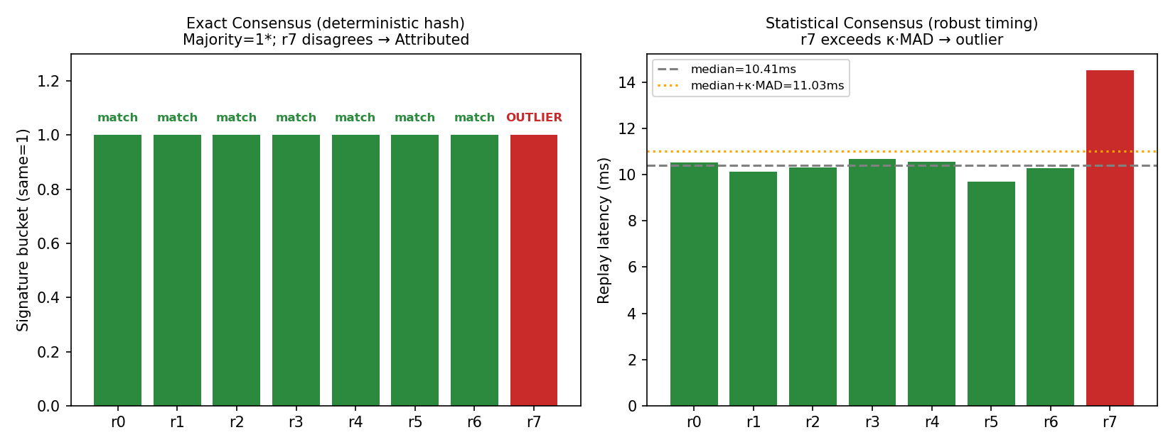
Lines 4–9: exact consensus. This branch handles evidence whose healthy value should be bit-for-bit identical across the whole peer group — progress coordinates, collective fingerprints, and the numerical hashes described above. SCOUT finds the most frequent value $e^*$ and its count $c^*$. If $c^* > N/2$ (a strict majority agrees), every rank whose evidence differs from $e^*$ is marked as an outlier. If no strict majority exists ($c^* \le N/2$), C3 refuses to guess and returns Inconclusive with an all-zero bitmap — this handles the case of multiple distinct minority values (e.g. two different corrupted ranks producing two different wrong answers) without falsely assuming there is exactly one faulty rank, and it deliberately declines to pick a winner in a two-rank tie.

Intuition and boundary: Exact consensus is explicitly not Byzantine fault tolerance and not a correctness oracle. It assumes the healthy value genuinely holds a strict majority. If a common-mode bug corrupts every replica identically (e.g., a software bug present in every rank’s code, not a hardware fault on one GPU), all ranks agree on the wrong answer, and C3 correctly reports Agree — because from C3’s local, relative perspective, there is no minority to attribute. This is a real, acknowledged blind spot: C3 detects divergence among peers, not absolute correctness.

Lines 10–15: statistical consensus. Execution timings among genuinely healthy peers will never be bit-identical (scheduling jitter, cache effects, etc.), so exact equality would produce false positives constantly. Instead, C3 computes the median $m$ of the peer timings and a robust scale $d$ (estimated primarily via the median absolute deviation, MAD $= \text{median}_i |\tau_i - m|$, falling back to interquartile range and then a scaled observed range if MAD is degenerate), then flags:

$$B[i] = \mathbb{1}\{ |\tau_i - m| > \kappa \cdot d \}$$

Why the median and MAD instead of mean and standard deviation? This is a deliberate, well-justified design choice. The mean and standard deviation are not robust — a single extreme straggler (say, one rank that hung for 30 seconds instead of taking 10ms) would massively inflate both the mean and the standard deviation, making the outlier detector less sensitive to exactly the fault it’s trying to catch (the classic “masking effect” in robust statistics). The median and MAD are robust to up to (just under) 50% contamination — consistent with the paper’s core assumption that faults are a minority. The paper cites Iglewicz & Hoaglin’s classic robust-statistics reference for this technique, which is the correct citation to make; this isn’t a novel statistical method, it’s a well-established robust estimator applied cleverly to the training-diagnosis setting.

The sensitivity multiplier $\kappa$ trades off false positives against detection sensitivity: a larger $\kappa$ requires a more extreme deviation before flagging, reducing false alarms but potentially missing subtle stragglers.

Line 12–13: the $d=0$ edge case. If every peer’s timing is bit-identical, $\text{RobustScale}$ returns exactly zero — there is no dispersion to measure a deviation against, so C3 short-circuits to Agree rather than dividing by zero or flagging spuriously.

Boundary condition, explicitly acknowledged by the paper: statistical consensus, by construction, will never flag a fleet-wide, simultaneous slowdown (e.g., a shared thermal or power event that slows down every peer in the group by the same amount) — because the median shifts along with the group, so no individual rank looks different from the (shifted) reference. The paper is explicit about this: “Statistical C3 intentionally misses a fleet-wide slowdown because no peer differs from the others.” Detecting that kind of degradation requires a temporal (historical) baseline, which SCOUT explicitly does not attempt to replace — a genuine and honestly stated scope boundary.

In-Situ Training Replay

Progress-coordinate comparison alone (comparing “which training step / layer index is rank X currently on”) can catch hangs, but it cannot catch a wrong numerical result or distinguish “genuinely slow computation” from “waiting on a dependency.” For that, SCOUT actually re-executes a sampled slice of the real computation — the layer forward/backward pass, or the optimizer update — on multiple equivalent peers, and compares the results via C3.

Algorithm 2: FSDP forward and replay (full pseudocode, unpacked)

Algorithm 2: Ordinary FSDP forward and SCOUT replay
Input:  Module M with shard θ_r; invocation x_r; shard group S_r;
        pre-forward RNG state ρ_r; equivalent peers G

1  Function FSDP(M, x_r, S_r):                  # normal (unmodified) forward
2      θ ← AllGatherParameters(S_r, θ_r)
3      y_r ← M(x_r, θ)
4      return y_r

5  Function Replay(M, x_r, S_r, ρ_r, G):          # SCOUT's diagnostic replay
6      (x, ρ) ← BroadcastSource(G, x_r, ρ_r)
7      R_broadcast ← C3((x, ρ), Exact, G)
8      (θ, t_gather) ← TimedAllGather(S_r, θ_r)
9      (y, t_M) ← TimedCall(M, Copy(x, θ))
10     R_coll ← C3(θ, Exact, G)
11     R_sdc ← C3(y, Exact, G)
12     R_gather ← C3(t_gather, Statistical, G)
13     R_module ← C3(t_M, Statistical, G)
14     return (R_broadcast, R_coll, R_sdc, R_gather, R_module)

Step-by-step, and why each line exists:

• Line 6, BroadcastSource: a module’s forward pass can take multiple input tensors (positional or named) plus a randomness state (e.g., for dropout). SCOUT designates one rank in the peer group as the source and broadcasts its captured input and RNG state to all peers. This is essential: without it, each peer would be replaying on different inputs (since DP/FSDP peers legitimately hold different data-parallel micro-batches), which would make any output difference meaningless — you’d be comparing apples to oranges, not detecting a fault.
• Line 7, R_broadcast: immediately verifies that the broadcast itself landed identically everywhere (defense against a corrupted broadcast, and a sanity check before doing expensive replay work).
• Line 8, TimedAllGather: re-does the real FSDP parameter materialization step, but timed — this produces $t_{\text{gather}}$, the AllGather communication latency, used for statistical consensus on communication timing.
• Line 9, TimedCall: runs the actual module forward on the broadcast (shared) input and the gathered (real) parameters, timed — this produces both the replay output $y$ (for numerical/SDC comparison) and $t_M$ (module compute latency, for statistical consensus on compute timing).
• Lines 10–11, R_coll and R_sdc: exact-consensus comparison of the materialized parameters (catches a corrupted parameter shard or a broken AllGather) and of the computed output (catches a corrupted compute unit — the classic SDC case).
• Lines 12–13, R_gather and R_module: statistical-consensus comparison of the two separately measured timings.

Design choice: why time communication and computation separately (not just total wall-clock)? This is one of the paper’s cleaner insights (Section 6.1.2, Figure 2 in the original). A straggler could be slow because its local compute is slow (a degraded SM or thermal throttling on that specific GPU) or because it’s waiting on a shared collective (e.g., a slow AllGather that synchronizes an entire FSDP shard group, in which case every member of that shard group will show elevated AllGather time, not just the culprit). If SCOUT only measured total time, these two very different root causes (and very different remedies — replace one GPU vs. investigate a network link) would be indistinguishable. By timing $t_M$ and $t_{\text{gather}}$ separately:

• An outlier in $t_M$ alone (module compute) directly identifies the straggling rank — no ambiguity, because compute happens locally.
• An outlier in $t_{\text{gather}}$ affects every member of that FSDP shard group symmetrically (because AllGather is a group-synchronizing collective) — it identifies the affected process group, not a single rank, which requires a further step (cross-PG validation, below) to pin down the actual machine.

Cross-PG validation: from “affected group” to “faulty machine”

If a communication straggler shows up as “the whole FSDP shard group $S_2 = \{r_4, r_5\}$ has elevated AllGather time,” SCOUT cannot yet tell whether $r_4$ or $r_5$ (or the network link between them) is at fault — both members see the delay symmetrically because AllGather synchronizes them. The paper’s solution is cross-PG validation: because a rank participates in multiple process groups simultaneously (e.g., both an FSDP shard group and a tensor-parallel group), if the tensor-parallel group also reports a straggler, and the two suspect sets from the two different process groups intersect at exactly one rank, that rank’s machine is the actual culprit.

Worked example from the paper: a 4×2 DP–FSDP mesh combined with TP degree 2 (16 ranks total, 2 TP slices). Suppose the FSDP shard group $\{r_4, r_5\}$ reports slow AllGather, and the TP group $\{r_4, r_{12}\}$ (same machine, since TP groups are typically confined within one machine due to TP’s heavy communication demands) also reports a slow collective. The intersection of $\{r_4, r_5\}$ and $\{r_4, r_{12}\}$ is $\{r_4\}$ — so SCOUT localizes the fault to the machine hosting $r_4$ (and $r_{12}$), not to an arbitrary member of either group.

This yields four distinguishable diagnoses depending on which combination of groups is slow:

1. Slow TP group and intersecting slow FSDP group → machine-local problem (replace this machine).
2. Slow TP group, normal FSDP group → intra-machine communication problem specific to the TP link.
3. Normal TP group, slow FSDP (inter-machine) group → inter-machine network problem; hand off to existing datacenter network diagnostics rather than trying to pin down link/switch-level detail SCOUT cannot see.
4. Many independent groups across many machines all slow, with no single machine explaining all of them → cluster-wide contention or a software issue, not a hardware fault.

This is a genuinely useful piece of engineering: it turns an ambiguous “this group is slow” signal into an actionable “replace this specific machine” or “escalate to network team” decision, using redundancy that’s already present in hybrid parallelism (a rank belongs to multiple orthogonal process groups) rather than requiring new instrumentation.

Out-of-Band Hang Localization

The above replay mechanism assumes the trainer is alive and progressing normally enough to schedule a replay. But a hang, by definition, means the trainer (and potentially its NCCL communicator) has stopped making progress — you cannot ask a frozen process to run a diagnostic replay.

Why communication hangs happen, and why the “first reporter” is unreliable evidence: the paper cites PyTorch’s own Flight Recorder analysis, which groups NCCL watchdog timeout causes into four categories: (1) CPU-side stalls or control-flow divergence, (2) a preceding GPU-kernel hang, (3) incompatible collective arguments (e.g., one rank issues a different-shaped collective than its peers expect), and (4) genuine network/hardware faults. Crucially, “almost all observed timeouts arise from desynchronization” — meaning the specific rank whose watchdog fires first and reports the timeout is often just the first bystander to notice, not the cause.

SCOUT’s solution: an independent, always-responsive observer. Each rank launches a separate CPU-only observer process. Training hooks publish a monotonic progress record (current optimizer step + an operation identifier at layer/DataLoader/collective boundaries) plus a “pending collective fingerprint” (process group, collective type, arguments) to local shared memory immediately before entering a potentially-blocking operation — critically, this publish happens before the rank enters the collective, so a lagging rank leaves behind a stale/different coordinate, while ranks already waiting inside the collective retain a later, matching coordinate. This ordering is what lets SCOUT distinguish “rank X never entered” from “ranks are all waiting together, victim of something else.”

These CPU observers talk to each other over an independently rendezvoused Gloo group — deliberately not the same NCCL communicator used for training — so that a frozen training-side GPU communicator cannot also freeze the diagnostic channel. This is the paper’s answer to “how do you diagnose a system that has stopped responding”: don’t put your diagnostic tool inside the thing that might freeze.

When the observer detects that visible progress has been silent beyond a configured threshold, it enters C3 with the gathered progress coordinates and collective fingerprints:

• If a minority of ranks show a different collective fingerprint or progress coordinate than the majority → rank-local software/control-flow divergence → recovery can restart the job in place on the same hardware (it’s likely a bug, not broken silicon).
• If all ranks report matching progress and fingerprints (everyone genuinely entered the same collective and is genuinely all waiting) → group-scoped runtime/transport stall → recovery should run hardware/fabric-level diagnostics, since the hang isn’t attributable to any one rank’s divergent behavior; it’s likely a network or device-level problem SCOUT’s evidence can flag but not further pinpoint.

MoE-Specific Extensions and Shape-Catalog Compression

Mixture-of-Experts models add a wrinkle: token routing is dynamic, so the “shape” of work each expert receives changes from batch to batch and step to step, unlike dense models where tensor shapes are fixed by configuration. Naively replaying every input shape an expert might see would be computationally prohibitive — the paper notes admitted shape spaces can contain “thousands of shapes.”

The key insight: coverage via execution-path dominance

Not every distinct input shape needs its own replay test, because many different shapes ultimately execute through the same underlying GPU kernel execution path (the same sequence of tile/kernel-scheduling decisions inside a grouped GEMM kernel). If shape $\alpha$ exercises every execution path that shape $\beta$ exercises, and does so at least as many times, then any persistent hardware fault detectable by replaying $\beta$ is also detectable by replaying $\alpha$ — so $\beta$ is redundant and can be skipped.

Formally, with an execution fingerprint $F(\alpha)$ (the kernel/scheduling configuration a shape triggers) and a path-count vector $\mathbf{c}(\alpha)$ (how many times each execution path is exercised):

$$\alpha \succeq \beta \iff F(\alpha) = F(\beta)\ \wedge\ \mathbf{c}(\alpha) \ge \mathbf{c}(\beta) \ \text{(componentwise)}$$

SCOUT computes, offline (before training starts, using the production expert kernel implementation on the target GPU/software stack), the minimum set of “representative” shapes whose coverage sets $C(\alpha) = \{\beta \mid \alpha \succeq \beta\}$ jointly cover every admitted shape. During training, SCOUT simply rotates through this small representative catalog rather than testing every shape.

Design choice discussion — why/alternative/boundary:

• Why: This directly targets the actual overhead bottleneck — exhaustive per-shape replay would make MoE diagnosis prohibitively slow, especially online.
• Alternative rejected: random sampling of shapes each round would be cheaper to implement, but gives no coverage guarantee — a persistent fault that only manifests under a rarely-sampled shape could go undetected indefinitely.
• Boundary, explicitly stated by the paper: this compression is only valid for a fixed hardware/software/kernel environment. Any environment drift (a new CUDA version, a new kernel implementation, a different GPU SKU) invalidates the catalog and requires offline rediscovery. It also only covers uniform per-expert row counts in the measured experiments; the paper explicitly states that “arbitrary heterogeneous routing vectors require separately qualified templates” — i.e., the neat compression numbers reported (see below) do not automatically generalize to every possible real-world routing skew pattern.

Algorithm 3: Checkpoint saving and retrieval

The final piece connects replay evidence to checkpoint correctness — because if SDC corrupts model or optimizer state, and that corrupted state gets checkpointed, restarting from “the latest checkpoint” reintroduces the corruption.

Algorithm 3: Checkpoint saving and retrieval
Input: Accepted-recipe count q=0; recipe-catalog size K;
       latest in-memory checkpoint CKPT_latest;
       current candidate CKPT_candidate; newest verified checkpoint CKPT_verified

1  Function CheckpointSave():
2      f ← job-wide SCOUT outcome
3      if f ∈ {SDC, Hang}:
4          return CheckpointRetrieval(f)
5      CKPT_latest ← newly captured in-memory checkpoint
6      q ← q + 1
7      if q = K:
8          q ← 0
9          CKPT_verified ← CKPT_candidate
10         persist CKPT_latest
11         CKPT_candidate ← CKPT_latest

12 Function CheckpointRetrieval(f):
13     if f = SDC  OR  ¬MachinesAccessible():
14         return CKPT_verified
15     if f = Straggler:
16         return CKPT_latest
17     R ← ReplayFullCatalog()
18     if HasSDC(R):
19         return CKPT_verified
20     return CKPT_latest

Why “promote after two consecutive clean cycles,” not one? This is a subtle but important detail (lines 7–11): a single accepted replay cycle only tests $K$ recipes at scattered points; a fault could corrupt training state after its triggering recipe already ran clean in that cycle, and that corruption would only be caught in the next cycle’s replay. So SCOUT only promotes a checkpoint to verified after two consecutive accepted cycles (comprising $2K$ checks total) — the first cycle’s checkpoint only becomes trusted once the second cycle’s full-catalog replay confirms nothing was silently corrupted in between.

The retrieval logic (lines 12–20) encodes exactly which failure modes require conservatism:

• Confirmed SDC, or a machine being physically inaccessible (so its shard can’t even be inspected) → fall back to the older, fully-verified checkpoint. Conservative, because you cannot trust that “latest” state.
• A straggler alone → use the latest checkpoint. Slowness by itself carries no numerical-corruption evidence, so there’s no reason to discard recent progress.
• Anything else (ambiguous/other failure) → run a full-catalog replay sweep as an emergency check; only fall back to verified if that sweep actually surfaces SDC evidence.

Experimental Evaluation

Setup

The evaluation runs on a genuinely modest testbed: two hosts, 8× NVIDIA A100-SXM4-40GB each, 16 training ranks total, connected via NVLink within a host and TCP (no RDMA) between hosts. The software stack is PyTorch 2.13.0, CUDA 13.0, NCCL 2.29.7, TorchTitan 0.2.2, Megatron-Core 0.18.2, DeepSpeed 0.19.4. Workloads are a deterministic three-block Transformer trained under DDP, FSDP2, and a 4×4 HSDP mesh, plus a broader integration matrix exercising pipeline/tensor/context/sequence/data/expert parallelism.

Fault-injection coverage (paper’s Table 3)

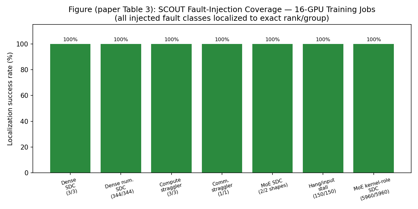
The headline numbers are genuinely strong on their own terms: across DDP/FSDP2/HSDP, all nine 16-GPU test cells for checkpoint recovery, SDC exclusion, and compute-straggler localization passed. In the dense numerical SDC sweep, 344/344 injected corruptions (including 64 deliberately “near-invisible” perturbations designed to be numerically subtle) were localized, and 30/30 fault-free control runs stayed clean (no false positives). In the largest test, MoE kernel-role SDC injections covering 5,960 selected execution-path occurrences all changed the observed output or gradient as expected, and persistent faults correctly localized the injected ranks (7 and 15) on both 8- and 16-GPU configurations.

What “coverage” means here, precisely, and why the caveat matters: these are injected software faults with known ground truth (a deterministic seed, a specific rank chosen ahead of time, e.g. “corrupt rank 9’s parameter after backward”), not naturally occurring physical failures observed in production. This is standard practice for validating a mechanism (you need ground truth to measure recall), but it means these numbers validate that the mechanism works as designed for the tested injection classes, not that SCOUT achieves some general “X% recall on real-world faults” — a distinction the paper itself is careful to state explicitly in its limitations section (quoted below).

MoE shape compression (paper’s Table 4)

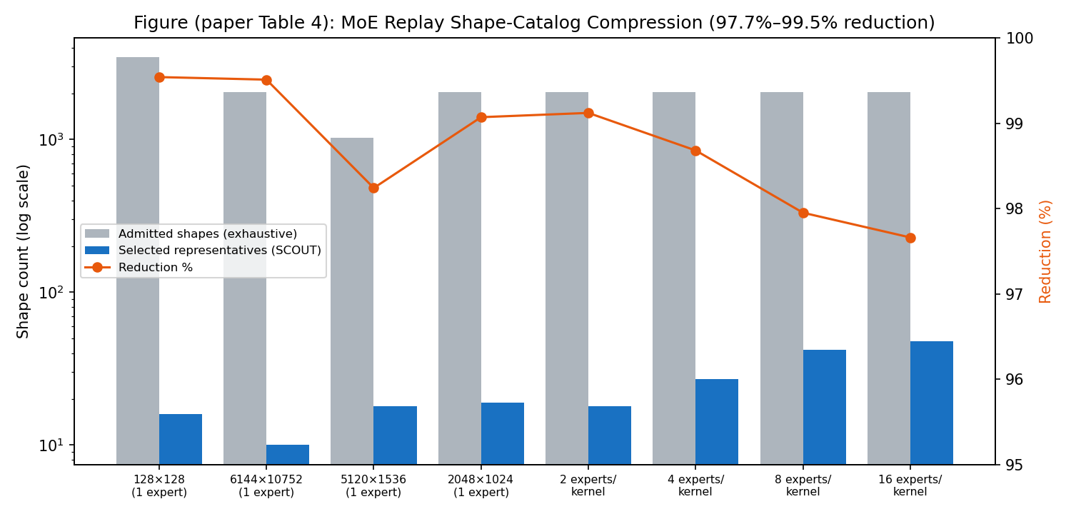
The compression results are the paper’s other headline number: a 128×128 single-expert projection admits 3,457 distinct shapes, compressed down to just 16 representatives (99.54% reduction) while still covering all 1,134,224 recorded execution-path occurrences across the admitted shapes. Grouped-kernel configurations (2–16 experts per kernel) retain proportionally more representatives (18–48 out of 2,048 admitted shapes) as more experts per kernel introduce more distinct pressure regimes — a sensible trend, since more concurrent experts means more distinct combinations of tile-scheduling decisions to cover.

Design-choice rationale reflected in the numbers

The overhead-budgeting math the paper provides is worth restating because it shows the authors thought carefully about why this system could plausibly run continuously in production without materially slowing training: for a model with $N$ repeated hidden layers, replaying one input variant through one hidden layer’s forward+backward costs roughly $1/N$ of one training iteration’s time. If SCOUT replays $V$ input variants once every $I$ iterations, the amortized overhead is approximately:

$$\frac{V}{I \cdot N}$$

For the paper’s example numbers ($V=3$, $I=20$, $N=50$): $3/(20 \times 50) = 0.3\%$ — a genuinely low estimated overhead, if this back-of-envelope model holds at production scale (see limitations below; the paper does not actually measure end-to-end throughput overhead empirically).

Related Work Positioning

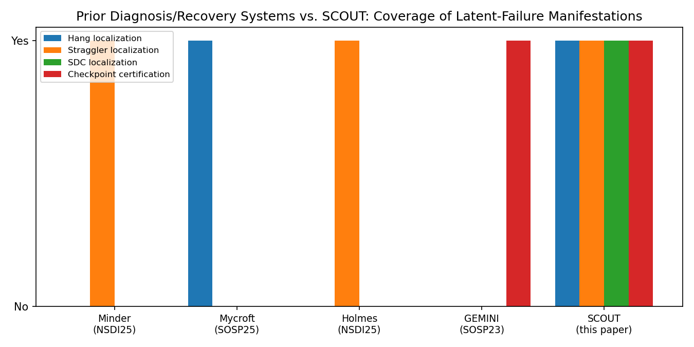
SCOUT sits in a crowded and increasingly mature space of LLM training resilience research (much of it from major industry labs like ByteDance, Meta, and NVIDIA collaborators — the reference list includes Minder, Mycroft, Aegis, Holmes, GREYHOUND, EROICA, TrainMover, TrainCheck, TrainVerify, AEGIS, SDCHunter, OpGuard, and GEMINI, among others). The paper is honest about how it complements rather than replaces these systems:

• Minder, Aegis: use job-level telemetry and diagnostic rules to detect faulty machines — SCOUT’s peer-consensus approach doesn’t need a pre-defined set of telemetry signals or fault-specific rules, but also doesn’t replace the operational infrastructure these systems provide.
• Mycroft: traces internal collective-communication state to reconstruct dependencies for hang localization — a complementary, lower-level view; SCOUT’s OOB observer operates at a higher abstraction level (progress coordinates and fingerprints, not raw collective internals).
• GEMINI: provides the actual in-memory checkpointing infrastructure that SCOUT’s checkpoint gate builds on top of — SCOUT is explicitly designed to be additive to GEMINI, not a replacement.
• AEGIS (the SDC paper, not to be confused with the “Aegis” fault-diagnosis system above — an unfortunate naming collision the field has produced), SDCHunter: also use replay-style evidence for SDC, but SCOUT’s specific contribution is tying completed, clean replay coverage to a checkpoint promotion protocol (Algorithm 3), rather than only using replay for detection.

Limitations (As Stated by the Authors)

The paper’s own “Discussion and Limitations” section is unusually candid, and worth quoting closely because it directly scopes what can and cannot be concluded from this work:

1. Evaluation scale is small. “The current evaluation exercises software fault injection and dense and MoE mechanisms on at most 16 A100 GPUs across two hosts.” The authors explicitly call for future work to “quantify detection accuracy, false positives, and time to evidence across multiple racks, hybrid-parallel layouts, and RDMA or multi-rail fabrics.”
2. No end-to-end throughput/overhead measurement. The 0.3% overhead figure is a theoretical estimate from a cost model, not a measured number from a production-scale run. The paper explicitly states it “does not measure end-to-end throughput and resource overhead across replay cadences, or report recovery time and rollback distance.”
3. Replay coverage is contractual, not universal. SCOUT “targets permanent faults and intermittent faults that recur under a similar operating regime; a one-shot fault that does not recur during replay falls outside this coverage contract.” A fault that happens once and never again during any scheduled replay window is invisible to this system by design.
4. MoE shape compression requires environment stability and uniform routing. As already discussed, arbitrary heterogeneous routing vectors are explicitly stated to require “separately qualified templates” not covered by the reported compression numbers.
5. Diagnosis scope is above the physical layer. SCOUT localizes to “an actionable rank, GPU, node, peer group, or conditionally an HCA/NIC endpoint” — it explicitly does not localize to a specific kernel instruction, cable, port, or switch; that requires handing off to external telemetry/fabric diagnostics.
6. Framework visibility gaps. “Public framework interfaces do not expose every collective launched inside FSDP, DTensor, fused kernels, or compiled graphs” — meaning some collectives are effectively invisible to SCOUT’s timing infrastructure unless version-specific adapters are written, and the current implementation “does not automatically time every parallel process group.”

Critical Analysis

This is the section where I want to push past what the authors already stated and add independent scrutiny, because a purely positive summary of any systems paper does a disservice to readers trying to decide whether to adopt or build on it.

(a) Weaknesses and flaws specific to this paper.

• Single-author, no institutional affiliation. The paper is authored solely by “Zhuang Wang, Independent Researcher.” This is unusual for a systems paper in this space (compare to the reference list, almost entirely multi-author papers from ByteDance, Meta-scale production teams, or well-resourced academic groups with cluster access). This doesn’t invalidate the technical contribution, but it plausibly explains limitation #1 (small evaluation scale) directly: an independent researcher very likely does not have access to a multi-thousand-GPU cluster to validate at the scale the motivating examples (MegaScale’s 12,288 GPUs, Llama 4’s 32,000 GPUs) describe. The gap between the motivation (failures at 10,000+ GPU scale) and the evaluation (16 GPUs, 2 hosts) is the single largest credibility gap in the paper, and while the authors are honest about it, it means the core claims about localization accuracy and overhead at the scale that actually matters remain unvalidated empirically, resting instead on the argument that the mechanism’s design should scale (majority voting doesn’t inherently require huge groups; overhead is amortized per-layer rather than per-GPU-count). That argument is plausible but not proven.
• The fault-injection methodology has a soft-confirmation bias built in. All reported injection experiments use a single deterministic seed and inject into a pre-selected, known rank (rank 9 or rank 15, repeatedly). The paper is transparent that “these software injections validate the mechanism and its stated localization scope, not recall over arbitrary physical failures” — but this also means we don’t know the false-negative rate under, say, randomized injection across many seeds and many rank choices, or under simultaneous multi-rank injection (which the paper’s own cited production evidence, ByteRobust, says is rare but not impossible — “one or two nodes” faulty, meaning sometimes two, and SCOUT’s exact-consensus rule explicitly cannot always distinguish two distinct minority values from each other in a small group).
• No comparison against a baseline detector in the same testbed. The paper cites Minder/Mycroft/Holmes/GREYHOUND as related work but never runs a head-to-head comparison on the same injected faults, even at the same modest 16-GPU scale, to show SCOUT actually localizes faster or more accurately than, say, a simpler heuristic (e.g., comparing raw per-rank iteration time against a fixed threshold). Without this, it’s hard to independently verify whether the sophistication of C3 (exact + statistical consensus, cross-PG intersection) is necessary versus whether a much simpler scheme would achieve comparable results on the tested fault classes.

(b) Limitations the authors understate or omit.

• The GPU kernel scheduling assumption behind MoE shape compression is fragile in a way the paper doesn’t fully explore. The compression relies on an execution fingerprint $F(\alpha)$ that is assumed stable for a “fixed training environment.” But GPU kernel autotuning (e.g., cuBLAS/cuDNN heuristics selecting different algorithms based on runtime conditions like current occupancy, not just static shape) can in principle select a different kernel implementation for the same shape depending on transient GPU state — the paper’s model implicitly assumes shape → kernel is a static, deterministic function, which is approximately true for many hand-tuned grouped GEMM kernels but is not guaranteed to hold for all backends, especially as kernel libraries evolve to use more adaptive/autotuned dispatch. This could silently invalidate the “coverage” guarantee in ways that would only surface as an undetected fault much later — precisely the failure mode SCOUT exists to prevent.
• Recovery-decision correctness is validated only at the mechanism level, not at the policy level. Algorithm 3’s checkpoint retrieval logic is logically clean, but the paper never tests scenarios where the combination of concurrent failure signals is ambiguous — e.g., what happens when a straggler and a suspected SDC are both flagged in overlapping recipe cycles, or when a machine becomes inaccessible mid-cycle (partial evidence)? Real production incidents are messier than clean, isolated injections, and the paper’s evaluation doesn’t probe this compositional complexity at all.
• The “additive, non-invasive” framing undersells real integration cost. The paper repeatedly emphasizes that SCOUT requires no training-loop or framework-source modification, which is true at the API level (enable_resiliency(...)), but building and maintaining the MoE shape catalog per hardware/software/model combination is real, recurring operational work that the paper’s cost model doesn’t account for — “environment drift invalidates the catalog and requires rediscovery” is stated as a limitation, but the actual frequency of environment drift in a production cluster running continuous integration/deployment of kernel libraries, driver updates, and model architecture changes is likely to be non-trivial, and re-running offline shape discovery at that cadence has a cost the paper never quantifies.

(c) Concrete, specific improvement suggestions.

1. Run a matched-baseline ablation. Even on the existing 16-GPU testbed, compare SCOUT’s C3-based localization time/accuracy against (i) a naive fixed-threshold per-rank timing detector and (ii) an ablation of SCOUT with cross-PG validation disabled, to isolate exactly how much of the reported accuracy comes from the “clever” parts of the design (robust statistics, cross-PG intersection) versus the basic majority-vote idea.
2. Test compositional/concurrent failure scenarios explicitly. Add injection experiments with two simultaneous, distinct faults (e.g., one straggler + one SDC in different peer groups at overlapping training steps) to validate Algorithm 3’s retrieval logic under realistic ambiguity, not just clean single-fault injections.
3. Quantify catalog re-discovery cost and drift frequency empirically, ideally by tracking how often a real production cluster’s driver/CUDA/kernel-library version actually changes over a representative multi-month window, and reporting the wall-clock cost of the offline shape-discovery procedure at the scale of a realistic MoE model (the paper’s Table 4 experiments appear to use a single instrumented Triton kernel on A100s — reporting this cost for, say, an H100/H200 cluster running a production-scale MoE model with hundreds of experts would substantially strengthen the practical-adoption case).

Reproducibility Notes

• Code: the paper states SCOUT is open source at https://github.com/LMResiliency/lm-resiliency — this is the concrete artifact to check for reproducing the fault-injection experiments.
• Frameworks needed: PyTorch 2.13.0, CUDA 13.0, NCCL 2.29.7, TorchTitan 0.2.2, Megatron-Core 0.18.2, DeepSpeed 0.19.4 (exact versions specified in the paper — a good sign for reproducibility, since NCCL/CUDA version drift is a known source of behavior changes in collective communication).
• Hardware: the full evaluation is reproducible on a comparatively modest 2-host × 8× A100-40GB setup (16 GPUs total), which is a genuinely accessible bar for an academic lab or well-resourced individual researcher to replicate, unlike papers requiring thousand-GPU access.
• What’s not reproducible from the paper alone: the exact fault-injection harness details (how faults are injected at precisely which point in the forward/backward graph) are described at a conceptual level (Table 3’s “injected trigger” column) but the actual injection code would need to come from the released repository to exactly reproduce the specific numbers in Tables 3–4.

Conclusion

SCOUT is a well-motivated, cleanly designed contribution to a genuinely important gap in LLM training resilience: localization, the step between “something is wrong” and “here is what to fix,” which prior checkpointing and restart mechanisms simply assume has already happened. Its core idea — using the redundancy that hybrid parallelism already creates (equivalent peer groups) as a source of “free” diagnostic evidence, compared via a single unified consensus primitive (C3) with both exact and robust-statistical modes — is elegant and generalizes cleanly across three quite different failure manifestations (hangs, stragglers, SDC). The cross-PG validation trick for turning “which group is slow” into “which machine is faulty” is a particularly nice piece of engineering that squeezes real diagnostic value out of structure the system already has, for free.

That said, the honest headline is: this is a promising mechanism validated at a scale two to three orders of magnitude smaller than the problem it’s motivated by. The paper’s own limitations section says as much, and a careful reader evaluating this for production adoption at genuine 10,000+ GPU scale should treat the reported 97–100% localization numbers as evidence the mechanism works as designed, not as evidence of production-scale recall, overhead, or robustness under the messier, compositional failure patterns that large real clusters actually produce.