HqeKV: Making Quantization and Eviction Cooperate Inside a Single KV Cache Compression Framework

Review date: 2026-08-26 Author: Zhongzhu Zhou Paper reviewed: HqeKV: Towards Hybrid Quantization and Eviction for KV Cache in Long-Context LLM Inference Paper authors: He Wang, Yu Gu, Fangfang Li, Zhigang Wang, Zhenghao Liu, Ning Wang, Xiaohua Li, Ge Yu (Northeastern University; Guangzhou University; Ocean University of China) arXiv: submitted to ACL Rolling Review, published as Findings of ACL 2026 (pages 4138–4153) Venue/Status: Findings of the Association for Computational Linguistics: ACL 2026

1. Why this paper is worth a careful read

If you have followed KV-cache compression for LLM inference over the last two years, you have probably noticed a strange pattern: the field has two well-developed toolboxes — quantization (KIVI, KVQuant, ZipCache, KVTuner, and a dozen variants) and eviction (H2O, SnapKV, StreamingLLM, PyramidKV, CAKE) — and until quite recently almost nobody combined them properly. Each toolbox on its own faces an unavoidable trade-off. Pure quantization keeps every token around but degrades all of them roughly uniformly, which wastes precision on tokens nobody will look at again. Pure eviction throws away entire tokens outright once they are judged unimportant, which is a much coarser and more destructive operation than shaving a few bits off a value. Neither strategy alone lets you spend your memory budget where it actually helps.

The obvious fix — “let’s do both” — has in fact been tried, but the paper argues (and I think correctly, based on the two prior works it cites, EvicPress and MiniKV) that earlier attempts to combine quantization and eviction were engineering-level stitches: pick an eviction ratio with one method, then quantize whatever survives with another method, without any principled way of deciding where the eviction/quantization boundary should sit or how many distinct precision levels to offer. HqeKV’s contribution is to treat the whole compression decision — which of five possible actions (FP16, three quantization precisions, or eviction) each cached key/value pair gets — as a single optimization problem with two coupled sub-problems: (a) how do you rank cached pairs by importance accurately enough to make five-way decisions instead of a binary keep/evict decision, and (b) once you have a ranking, how do you decide the boundaries between the five tiers so that the aggregate compression hits a memory target while minimizing quality loss?

This review will walk through both sub-problems in detail, because they are where the real technical content lives: a derivation connecting quantization error to the range of a cached vector (Section 3.2 of the paper), a joint K–V importance metric built on that derivation, a Tree-structured Parzen Estimator (TPE) based search for the precision-ratio boundaries, and a decoding-time re-quantization heuristic that keeps the whole system cheap enough to run in an inference-serving loop. I will also spend real time on where the paper’s evidence is thinner than its headline numbers suggest — the offline calibration dependency, the single-GPU/single-model-family experimental scope, and a few places where the “5 actions per cached pair” framing may be doing more marketing work than the ablations can support.

2. Prerequisites

2.1 Transformer self-attention and why KV cache exists

A decoder-only Transformer layer processes an input sequence by first projecting each token’s hidden vector into three role-specific vectors: a query $Q$, a key $K$, and a value $V$. Self-attention output for a given head is computed as

$$O = \text{Softmax}\left(\frac{QK^\top}{\sqrt{d_h}}\right) V, \tag{1}$$

where $d_h$ is the per-head dimension. Intuitively: the query of the current token is compared (dot product) against the keys of every token in the sequence, producing a similarity score per pair; softmax turns those scores into a probability distribution (“attention weights”); and the output is a weighted average of the value vectors, weighted by those attention probabilities. This is the mechanism that lets a token “look back” at earlier tokens and pull in relevant information from them.

Autoregressive generation computes this operation once per new token, and — crucially — the keys and values of all previously generated tokens are the same at every generation step; only the query changes. Recomputing $K$ and $V$ for the whole prefix at every single decoding step would be a wasteful $O(n^2)$ ballooning of the cheapest possible decoding loop, so essentially every production LLM serving stack instead caches the keys and values of tokens already processed. When token $x_{t+1}$ is generated, its key $k_{t+1}$ and value $v_{t+1}$ get projected once and appended to the cache: $K \leftarrow [K \mid k_{t+1}]$, $V \leftarrow [V \mid v_{t+1}]$. This is the “KV cache,” and it is what makes decoding an incremental $O(n)$-per-step operation instead of $O(n^2)$.

The catch: the KV cache’s memory footprint grows linearly with sequence length, and for long-context applications (100K+ token prompts, multi-turn agents, RAG pipelines with large retrieved contexts) it can dwarf the model’s own weight memory. This is the concrete problem HqeKV — and the entire “KV cache compression” literature — is trying to solve.

2.2 Two families of compression: quantization and eviction

Quantization reduces the numerical precision used to store each cached value — e.g., storing a 16-bit floating-point number as a 4-bit, 2-bit, or even 1-bit integer plus a small amount of shared metadata (a scale and offset). Every token is kept, but every token loses some fidelity. Eviction instead keeps a subset of tokens at full precision and discards (“evicts”) the rest entirely — usually the tokens judged least likely to be attended to again. Neither preserves the original information perfectly; the design question is really about where you want to accept information loss, and how granular your loss-budget control can be.

The paper’s core claim about prior integration attempts (EvicPress, MiniKV) is that they pick a fixed, coarse set of compression actions and largely bolt existing single-technique pieces together, rather than jointly optimizing the boundary between “quantize this token to precision level $p$” and “evict this token” over a continuous, more expressive action space.

2.3 Uniform vs. normalized quantization

HqeKV uses two different low-level quantization schemes and picks between them per precision level. Uniform quantization maps a real-valued vector $\Xi \in \mathbb{R}^{1\times D}$ to $b$-bit integers by dividing its observed range into $2^b$ equal-width bins:

$$\Xi_q = \frac{\Xi - z}{s}, \qquad \Xi_{dq} = \Xi_q \cdot s + z, \tag{2}$$

where $z = \min(\Xi)$ is the offset and $s = \frac{\max(\Xi) - \min(\Xi)}{2^b - 1}$ is the scaling factor (bin width). Each real number gets rounded to the center of its nearest equal-width bin — this is the standard “affine” or “asymmetric” quantization used almost everywhere in the quantization literature.

Normalized quantization instead assumes the data follows (approximately) a Gaussian distribution — which prior work (NQKV, cited in the paper) has empirically verified holds for KV-cache activations — and places bin boundaries at the quantiles of a standard normal distribution rather than at equal intervals of the raw range:

$$\Xi' = \frac{\Xi - m}{s}, \tag{3}$$

where $m$ and $s$ are the empirical mean and standard deviation of the vector. Then bin centers $C = [c_0, \dots, c_{2^b - 1}]$ are placed at the $\frac{1}{2^b}, \dots, \frac{2^b-1}{2^b}$ quantiles of the standard normal density, and each value is assigned to whichever bin’s cumulative-probability mass integral is smallest:

$$\Xi_{i,q} = \arg\min_{0 < j < 2^b - 1} \int_{\min(c_j, \Xi'_i)}^{\max(c_j, \Xi'_i)} \phi(u)\,du, \tag{4}$$

with $\phi$ the standard normal density. Intuitively: since Gaussian mass concentrates near the mean, normalized quantization places more bins near the mean and fewer bins in the tails — a form of density-aware, non-uniform binning, whereas uniform quantization spends bins evenly across the observed range regardless of where the actual data mass sits.

Why maintain both schemes instead of picking a winner? Because — and this is one of the paper’s genuinely useful small findings — which scheme wins depends on the bit-width, a point I return to in Section 3.4.

3. The core idea: five-way compression as a ranking + boundary problem

3.1 System overview

HqeKV runs inside a single Transformer layer’s KV-cache handling logic (Figure 1 in the paper illustrates one layer). During prefilling, $Q$, $K$, $V$ are generated for the initial prompt; a joint importance metric (Section 3.2 below) is computed for every cached key/value pair; a search-based optimizer (Section 3.3) determines what fraction of cached pairs should receive each of five treatments — FP16 (no compression), 4-bit quantization, 2-bit quantization, 1-bit quantization, or eviction; and precision-specific quantization strategies (Section 3.4) then execute those decisions, applying uniform quantization at 4/2-bit and normalized quantization at 1-bit. During decoding, the cache is periodically re-quantized (Section 3.5) as new tokens accumulate and importance rankings shift.

flowchart LR
    subgraph Prefill["Prefilling Phase"]
        A["Input tokens"] --> B["Q, K, V projections"]
        B --> C["Joint K-V Importance Metric<br/>(attention weights x V-range)"]
        C --> D["TPE Search:<br/>optimal boundary ratios<br/>delta1..delta4"]
        D --> E["Assign 5 actions:<br/>FP16 / 4-bit / 2-bit / 1-bit / evict"]
    end
    E --> F["Compressed KV Cache<br/>(mixed precision, packed)"]
    subgraph Decode["Decoding Phase (every T tokens)"]
        F --> G["Update running importance<br/>(attention window + range)"]
        G --> H["Re-quantize:<br/>only downgrade precision,<br/>never upgrade"]
        H --> F
    end
    F --> I["Attention computation<br/>with dequantized K,V"]

Figure 1 (architecture, reproduced from paper Fig. 1 description): HqeKV’s per-layer pipeline — a single importance metric feeds a search-based allocator that assigns one of five compression actions per cached pair, followed by a periodic decoding-time re-quantization loop.

My first reaction reading this: the five-way action space is the paper’s central design bet, and it is a sensible one if and only if the importance ranking that drives the boundary decisions is accurate — because a five-way split amplifies the cost of ranking errors relative to a coarse binary keep/evict split. A token mis-ranked into “evict” when it should have been “4-bit” costs you the entire token; a token mis-ranked between two adjacent quantization tiers costs you a few bits of precision. So the burden on Section 3.2’s importance metric is higher here than in prior eviction-only work, and it’s worth checking whether the paper’s metric actually clears that higher bar (I look at this in Section 6.2).

3.2 Why range predicts quantization error — and the joint K-V importance metric

The problem prior metrics have. Almost all cited eviction and quantization-selection methods (H2O, SnapKV, PyramidKV) rank tokens by cumulative attention weight — essentially, “how much attention has this token historically received.” This is a reasonable proxy for the key vector’s importance, since attention weights are literally computed from $K$. But it structurally ignores the value vector $V$ entirely, even though $V$ is what actually gets averaged into the output (Equation 1). A token could receive moderate attention weight but carry a value vector with an unusually large dynamic range — and if that vector is aggressively quantized, the resulting output error could be disproportionately large precisely because the range is large, independent of the attention weight.

Deriving the range–error relationship. The paper’s most substantive piece of theoretical work is a derivation connecting the expected quantization error of a vector to its observed range. Assume the values to be quantized are drawn i.i.d. from a distribution $p(\xi)$, and denote by $c_i$ the quantization center of interval $I_i$ (one of $2^b$ intervals). The expected squared quantization error over the interval $[\min(\Xi), \max(\Xi)]$ is:

$$\mathbb{E}_{\xi \sim p(\xi)}\Big(L_n(\xi) \mid \xi \in [\min(\Xi), \max(\Xi)]\Big) = \frac{\sum_{i=0}^{2^b - 1} \int_{\xi \in I_i \cap [\min(\Xi), \max(\Xi)]} (\xi - c_i)^2\, p(\xi)\, d\xi}{\int_{\min(\Xi)}^{\max(\Xi)} p(\xi)\, d\xi}. \tag{5}$$

Let’s unpack this carefully, because it’s easy to gloss over as “just an expectation formula.” The numerator sums, over every quantization interval, the probability-weighted squared distance between a sampled point and that interval’s representative codeword — this is the standard mean-squared-error decomposition for any quantizer. The denominator normalizes by the total probability mass actually falling inside the observed range (a technical correction since we’re conditioning on the vector’s realized min/max rather than the full support of $p$). The key move is architectural, not just mathematical: this expression is deliberately written to be agnostic to whether the quantizer is uniform or normalized — the distinction between the two schemes shows up only in how the intervals $I_i$ are drawn and where the codewords $c_i$ sit, not in the functional form of the error. That is what lets the paper claim the range–error relationship holds for both quantization families it uses.

From here, the paper’s argument is: since Equation (5) shows the error is entirely a function of where $\xi$ falls relative to the interval boundaries, and the interval boundaries are themselves derived from $[\min(\Xi), \max(\Xi)]$, the vector’s range $R_\Xi = \max(\Xi) - \min(\Xi)$ is a first-order proxy for how much quantization error the vector will incur — wider range means each fixed-width (or fixed-quantile) bin has to cover more numerical territory, so any single value’s distance to its assigned codeword grows. This is intuitively obvious for uniform quantization (bin width is literally $R_\Xi / (2^b-1)$, so error scales linearly with range for a fixed bit count) but the paper additionally verifies it holds empirically for normalized quantization, where the relationship is less mechanically obvious since bin placement depends on the normal quantile function rather than the raw range directly.

Empirical validation. The paper numerically integrates Equation (5) under 4-bit uniform quantization assuming $p(\xi)$ is a standard normal density (Figure 2a in the paper), and separately measures actual conversion losses on 1,000 real tokens sampled from a Llama-3.1-8B-Instruct KV cache on a LongBench question, quantized at 4-bit, 2-bit, 1-bit uniform, and eviction (Figure 2b, Table 1). The reported Pearson correlation coefficients between range and conversion loss are strikingly high — 0.96 at 4-bit, 0.96 at 2-bit, 0.95 at 1-bit, and 0.91 for eviction — versus 0.88, 0.88, 0.84, 0.73 respectively for randomly generated Gaussian vectors of the same dimensionality. The fact that the correlation is higher on real KV-cache data than on synthetic Gaussian data is a nice touch: it suggests the range signal is not an artifact of assuming Gaussianity but genuinely reflects structure present in real cached activations.

xychart-beta
    title "Illustrative Relationship: Range vs. Quantization Error (Eq. 5 intuition)"
    x-axis "Vector range R" [0.5, 1.5, 2.5, 3.5, 4.5, 5.5]
    y-axis "Expected squared error (arb. units)" 0 --> 25
    line "1-bit (2 levels)" [2, 8, 20, 22, 24, 25]
    line "2-bit (4 levels)" [0.5, 2, 5, 9, 15, 22]
    line "4-bit (16 levels)" [0.1, 0.3, 0.7, 1.2, 2, 3]

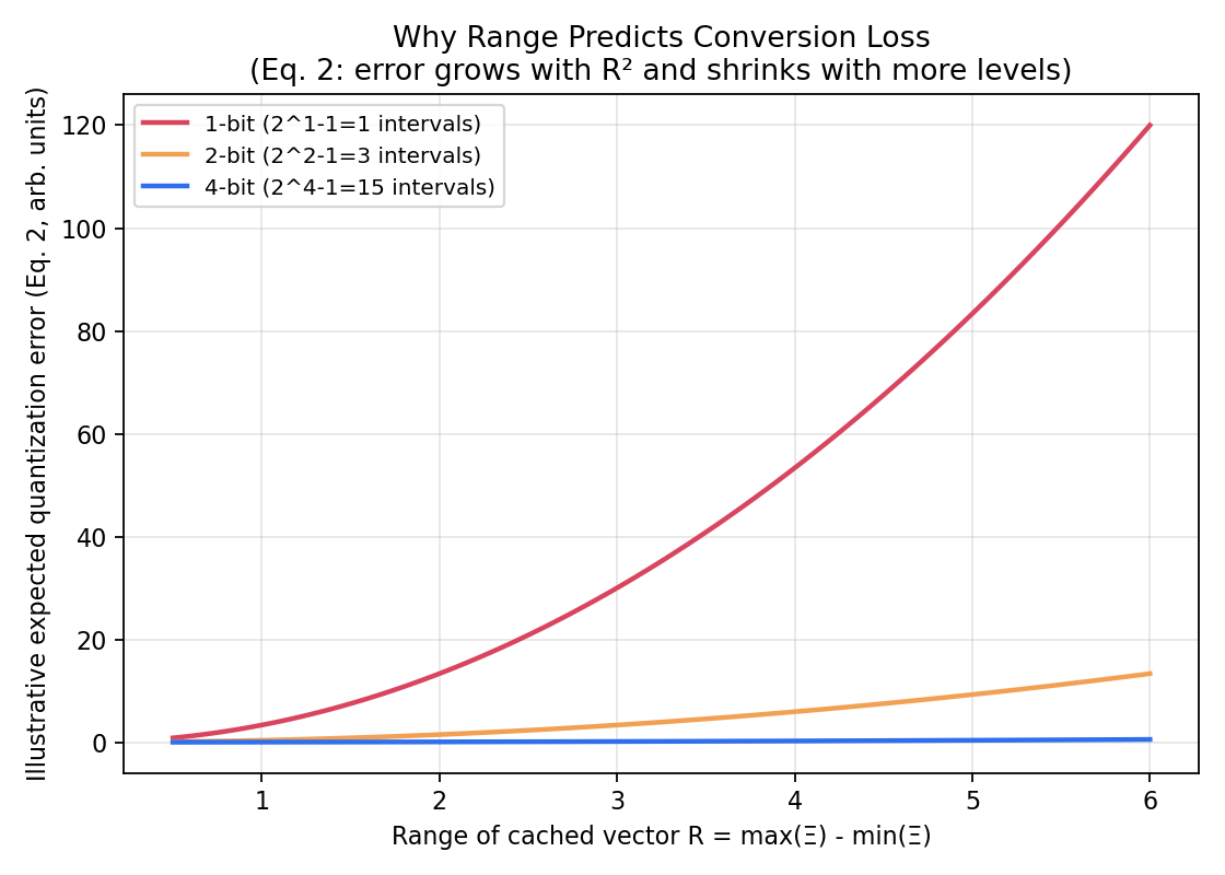
Figure 2 (math-visualizing figure, my own reconstruction of the Eq. 5/Table 1 intuition): at any fixed bit-width, expected quantization error grows roughly with the square of the vector’s range, while doubling the bit count (more quantization levels) suppresses that growth substantially — this is exactly the qualitative shape behind the paper’s Pearson correlation results in Table 1.

I generated a cleaner standalone version of this relationship for the review (not copied from the paper, which only shows a numerically-integrated curve and a scatter plot):

Building the joint metric. With the range–error link established, the joint importance metric is straightforward to state, though its motivation took the derivation above to earn:

• Key importance = cumulative attention weight (unchanged from prior work — this remains a reasonable signal for $K$ specifically, since attention weights are literally a function of $K$).
• Value importance = cumulative attention weight multiplied by the range of the corresponding value token: $\text{metric}_V = \text{metric}_K \odot \text{Range}(V)$.

The multiplicative combination is a deliberate reading of Equation (1): since the attention output is a weighted sum $\sum_i A_i V_i$, a token’s contribution to output error under $V$-quantization scales with both how much attention weight it receives ($A_i$) and how much quantization error its $V_i$ will incur (which, per the derivation above, scales with $V_i$‘s range). Multiplying the two signals together directly targets “how much output-level damage will quantizing this specific token’s value do,” rather than treating attention weight and range as independent, separately-thresholded criteria.

Design-choice discussion. Is multiplication the right combination rule? The alternative would be something like a weighted sum ($\alpha \cdot A_i + \beta \cdot \text{Range}_i$) or a max/min combination. The paper doesn’t ablate this choice explicitly, which is a gap — a weighted-sum formulation with tunable $\alpha, \beta$ could in principle adapt better across tasks with very different attention-weight and range distributions, whereas a pure product is scale-sensitive (if either factor happens to be numerically small across the board for a given layer or head, the product could collapse the dynamic range of the joint metric and make downstream ranking noisy). The multiplicative choice is also the most literal reading of Equation (1)‘s structure, so it has strong first-principles justification, but “first-principles-motivated” and “empirically validated as the best of several alternatives” are different claims, and only the former is demonstrated here.

3.3 The optimizer: turning a ranking into five-way boundaries

Having a ranking is necessary but not sufficient — you still need to decide how many tokens go into each of the five buckets (FP16 / 4-bit / 2-bit / 1-bit / evict) to hit a target average bit-width while minimizing quality loss. Let $\delta_1, \delta_2, \delta_3, \delta_4$ denote the ratios of cached pairs assigned to 4-bit, 2-bit, 1-bit, and eviction respectively (the remainder, implicitly, stays FP16). Given a target average bit-width $B_{avg}$, the ratios must satisfy:

$$\begin{cases} 4\delta_1 + 2\delta_2 + \delta_3 = B_{avg} \\ \delta_1 + \delta_2 + \delta_3 + \delta_4 = 1 \end{cases}, \quad \text{s.t. } B_{avg} > 0,\ 0 \le \delta_1, \dots, \delta_4 \le 1. \tag{6}$$

This is two linear equations in four unknowns, so it has infinitely many solutions — a 2-dimensional solution family, not a single point. The paper’s approach: pick $\delta_3, \delta_4$ as the two free variables, solve for $\delta_1, \delta_2$ in terms of them algebraically, and then search over $(\delta_3, \delta_4)$ using the Tree-structured Parzen Estimator (TPE), a Bayesian-optimization technique from the hyperparameter-tuning literature (Bergstra et al., 2011) that builds two probabilistic models — one for “good” hyperparameter regions and one for “bad” ones — and samples new candidates that are more likely under the good model relative to the bad model. This is exactly the same algorithm underlying tools like Optuna’s default sampler.

Why TPE instead of grid search or manual thresholds? The paper frames the earlier baselines’ “manual allocation or fixed thresholds” as the thing to beat. TPE has a real advantage here: a grid search over a continuous 2D space at fine resolution is expensive (you’d need to re-run inference over the calibration set at every grid point), while TPE adaptively concentrates its sampling budget in promising regions after a handful of exploratory iterations, making 200 total evaluations plausible. The obvious alternative not discussed is a gradient-based or differentiable relaxation of the boundary-selection problem (e.g., a Gumbel-softmax over the five actions) — this could in principle be far cheaper than 200 discrete black-box evaluations, but would require making the eviction/quantization pipeline end-to-end differentiable, which the paper’s Triton-kernel-based hard-boundary implementation is not designed for. TPE is the pragmatic choice given that constraint, not necessarily the theoretically optimal one.

The full search procedure (Algorithm 1 in the paper, reproduced and explained):

1. Initialize minimum loss $L \leftarrow \infty$ and optimal ratio list $R_{opt} \leftarrow \{\}$.
2. Load a calibration input $S$ (the paper uses a 16K-token slice of WikiText-2) and compute its full-precision prefilling output $F \leftarrow \text{LLM}(S)$ — this is the “ground truth” the search is trying to stay close to.
3. For 200 iterations: a. Sample candidate free variables $x_3, x_4$ from the TPE proposal distribution. b. Algebraically recover $x_1 = B_{avg} - 2 + x_3 + 2x_4$ and $x_2 = 4 - B_{avg} - 3x_3 - 4x_4$ (these come directly from solving Equation 6 for $\delta_1, \delta_2$ given $\delta_3=x_3, \delta_4=x_4$). c. If $x_1 < 0$ or $x_2 < 0$ (an infeasible ratio combination), set the loss to $\infty$ for this candidate — a simple rejection mechanism rather than a projected/clipped feasible search. d. Otherwise compute the candidate loss $L_{temp} = \mathcal{L}(F, \text{LLM}(S, R)) + L_{reg}$, where $\mathcal{L}$ is cross-entropy between the full-precision and compressed-precision prefilling outputs on the calibration set, and $L_{reg} = \alpha x_3 + \beta x_4$ is a regularization term that explicitly penalizes using more low-precision (1-bit) or eviction actions, nudging the search away from degenerate all-eviction or all-1-bit solutions even if they happen to minimize calibration-set cross-entropy. e. If $L_{temp} < L$, update the running best. f. Feed $(L_{temp}, x_3, x_4)$ back to the TPE sampler to update its proposal distribution for the next iteration.
4. Return $R_{opt}$.

One implementation detail worth flagging explicitly because it materially affects the accuracy of the final allocation: the paper doesn’t rank individual tokens, it ranks chunks. The KV cache is partitioned into groups of size $G$ (set to 32 in the experiments), and a chunk’s importance is the average importance of the tokens inside it. This is presumably done for computational tractability (searching over per-token boundaries at the granularity of individual cache entries would make the calibration loop far more expensive and the resulting compression map far more irregular to execute efficiently), but it does mean that within a chunk of 32 tokens, a single very-high-importance token sitting next to 31 unimportant ones will have its true importance diluted by averaging — a genuine information loss relative to per-token decisions, traded off against tractability and kernel efficiency. The paper additionally always keeps the top-2 most important chunks in full FP16 precision regardless of what the search recommends, an empirical safety margin rather than something derived from the optimization itself.

3.4 Why the “right” quantization strategy depends on bit-width

This is the paper’s second interesting empirical finding, and it’s a genuinely non-obvious one: uniform quantization is better at high bit-widths, normalized quantization is better at low bit-widths, and the crossover happens somewhere around 2-bit.

The evidence (Table 2, real KV-cache data from Llama-3.1-8B-Instruct on a Qasper question in LongBench; Table 3, synthetic Gaussian vectors as a sanity check):

Strategy	K @4-bit	K @2-bit	K @1-bit	V @4-bit	V @2-bit	V @1-bit
Uniform	5.28	25.59	92.06	0.29	1.44	4.67
Normalized	9.28	23.29	37.44	0.62	1.47	2.05

At 4-bit, uniform quantization has lower conversion loss for both K and V; at 1-bit, normalized quantization wins decisively (37.44 vs. 92.06 for K; 2.05 vs. 4.67 for V), with 2-bit sitting in an ambiguous middle zone where the two strategies are close. The same reversal pattern shows up on purely synthetic Gaussian vectors (Table 3), which rules out the possibility that this is some quirk specific to Llama’s activation statistics — it’s a property of how the two quantization schemes interact with bit-width, independent of the specific model.

Why does this happen, mechanistically? Uniform quantization spreads its limited number of bins evenly across the observed range, including the tails; at low bit-widths (few bins total), this wastes precious bins on rarely-occupied tail regions, leaving too few bins to resolve the densely-populated center where most of the actual data mass sits. Normalized quantization, by placing bins at Gaussian quantiles, concentrates resolution where the data actually is — a clear win when bins are scarce (1-bit: only 2 possible codewords, so where you place them matters enormously). At high bit-widths (4-bit: 16 codewords), there are enough bins that both strategies can adequately cover the dense center and have some bins left for the tails, so the intrinsic simplicity and lower per-value computational cost of uniform quantization’s fixed bin width wins out — normalized quantization’s more complex quantile-lookup and probability-integral computation (Equation 4) doesn’t buy enough accuracy improvement to justify itself.

HqeKV’s resulting design choice: apply uniform quantization at 4-bit and 2-bit, normalized quantization at 1-bit. This is a sensible policy read directly off the crossover point in the empirical tables, though I’d flag it as somewhat under-motivated as a general rule — the crossover point (roughly 2-bit) was identified on one model family (Llama-3.1-8B) and one dataset slice; whether the exact crossover point shifts for models with different activation statistics (e.g., models using different normalization schemes, or with substantially different KV head dimensions) is not tested. The paper does at least also run Qwen3-8B in its main experiments (Table not fully reproduced above but referenced), which provides modest cross-model support even if the bit-width-strategy crossover specifically isn’t re-verified there.

3.5 Decoding-phase strategy: periodic, one-directional re-quantization

A subtlety of decoding is that token importance rankings change over time — a token that looked unimportant during prefilling might accumulate more cumulative attention weight as generation proceeds, and vice versa. Re-computing the full boundary search after every single generated token would be prohibitively expensive (each TPE iteration requires a forward pass through the calibration set). HqeKV’s compromise: re-quantize the entire cache every $T$ generated tokens ($T=32$ in experiments, matching the chunk size $G$), and within a re-quantization event, only allow tokens to move to a lower precision, never a higher one.

This one-directional rule is justified empirically rather than theoretically: Table 7 in the appendix shows that across all measured transitions on a DuReader question, the fraction of KV-cache entries that would have moved from lower to higher precision (i.e., importance increased enough to warrant an upgrade) is tiny — 1.18% for 1→2-bit and 2.16% for 2→4-bit on the Key cache, similarly small on the Value cache, and exactly 0% for 4-bit→FP16 transitions in both K and V. The design choice trades a small, empirically-bounded amount of missed precision upgrades for a meaningfully simpler and cheaper decoding-time algorithm (Algorithm 3 in the paper): you never need to “restore” evicted or heavily-quantized information, which avoids having to keep a full-precision shadow copy of everything just in case a later upgrade is needed.

Boundary case worth flagging: the “never restore” policy means that a token evicted early in a long generation, which later becomes critically relevant (e.g., a fact referenced again much later in a long agentic trajectory), is permanently gone — there is no recovery path. For short-to-medium contexts where the 1.18-2.16% upgrade-transition rate was measured, this is a fine trade-off; for very long, non-monotonic attention patterns (e.g., a needle-in-a-haystack scenario where an early token becomes critical only much later), the empirical justification (measured on one DuReader question) may not transfer, and this is exactly the kind of boundary condition the paper’s Limitations section does not explicitly discuss (see Section 6).

3.6 How HqeKV positions itself against prior integration attempts

flowchart TB
    subgraph SingleCoarse["Single action family, coarse"]
        A1["H2O / StreamingLLM<br/>fixed evict threshold"]
        A2["KIVI / OTT<br/>uniform 2-bit for all tokens"]
    end
    subgraph SingleFine["Single action family, fine-grained"]
        B1["ZipCache / KVTuner<br/>mixed-precision quantization only"]
        B2["CAKE<br/>layer-aware eviction only"]
    end
    subgraph HybridCoarse["Hybrid family, coarse boundary"]
        C1["MiniKV / EvicPress<br/>bolted-on quant+evict,<br/>fixed/manual thresholds"]
    end
    subgraph HybridFine["Hybrid family, fine-grained (target zone)"]
        D1["HqeKV<br/>5-way action space,<br/>TPE-searched boundaries,<br/>joint K-V importance metric"]
    end
    SingleCoarse -."add mixed precision".-> SingleFine
    SingleCoarse -."add eviction option".-> HybridCoarse
    SingleFine -."add eviction option".-> HybridFine
    HybridCoarse -."add principled boundary search".-> HybridFine

Figure 6 (baseline/prior-art comparison, my own construction from the paper’s related-work discussion in Section 5): existing methods cluster either in “single action family” (pure quantization or pure eviction, regardless of how finely they subdivide bit-widths) or “hybrid but coarse” (MiniKV, EvicPress bolt existing pieces together without a principled boundary search). HqeKV’s claimed contribution is to be simultaneously hybrid (5 actions) and fine-grained (TPE-searched boundaries rather than fixed thresholds) — the quadrant no prior cited method fully occupies. This positioning is a reasonable reading of the paper’s own framing in Section 5, though as discussed in Section 6, the fine-grainedness is itself bounded by chunk-level (not token-level) decisions.

3.7 A worked numeric example: from bit-width target to per-token action

It’s easy to lose the concrete mechanics of Sections 3.2-3.3 in the notation, so here is a small worked-through example showing how HqeKV would treat a toy 8-token chunk.

Suppose we have a chunk of $G=8$ cached key/value pairs (in reality $G=32$, but 8 keeps the arithmetic legible), with cumulative attention weights (importance for K) and value-vector ranges as follows:

Token	Cumulative attn. weight $A_i$	Value range $R_i$	Joint metric $A_i \times R_i$
$t_1$	0.42	0.8	0.336
$t_2$	0.05	3.1	0.155
$t_3$	0.31	1.2	0.372
$t_4$	0.02	0.5	0.010
$t_5$	0.38	2.4	0.912
$t_6$	0.01	4.2	0.042
$t_7$	0.09	0.3	0.027
$t_8$	0.44	1.5	0.660

Ranking tokens by the joint metric (highest first, per Section 3.2): $t_5 (0.912) > t_8 (0.660) > t_3 (0.372) > t_1 (0.336) > t_2 (0.155) > t_6 (0.042) > t_7 (0.027) > t_4 (0.010)$.

Now suppose the TPE search (Section 3.3) has converged on ratios $\delta_1=0.25$ (4-bit), $\delta_2=0.25$ (2-bit), $\delta_3=0.25$ (1-bit), $\delta_4=0.25$ (evict) for this target $B_{avg}$ — a deliberately even split for illustration. Applying these ratios to our 8-token chunk (2 tokens per tier), the highest-ranked pair $\{t_5, t_8\}$ gets 4-bit uniform quantization, the next pair $\{t_3, t_1\}$ gets 2-bit uniform quantization, the next pair $\{t_2, t_6\}$ gets 1-bit normalized quantization (note the strategy switch per Section 3.4), and the lowest pair $\{t_7, t_4\}$ is evicted entirely.

Notice something instructive here: $t_6$ has the lowest raw attention weight in the chunk (0.01) but survives into the 1-bit tier rather than being evicted, purely because its value range (4.2, the largest in the chunk) inflates its joint metric relative to $t_7$‘s. This is exactly the scenario the joint K-V metric is designed to catch and that a K-only metric (cumulative attention weight alone) would get wrong — a pure attention-weight ranking would have evicted $t_6$ and kept $t_7$, when in fact $t_6$‘s large value range means quantizing (rather than evicting) it preserves more usable signal per bit spent. This is a small but concrete illustration of why the paper’s Section 3.2 derivation earns its keep: it changes which tokens actually get evicted, not just how finely graded the quantization is.

3.8 Putting the pieces together: a full compression cycle in prose

Before moving to the experiments, it is worth stating the entire prefilling-to-decoding compression cycle as a single connected narrative, since Sections 3.2 through 3.5 each cover one piece in isolation.

When a new request arrives, the prompt is processed once through the model to produce initial $K$ and $V$ caches (prefilling). Immediately after this pass, HqeKV computes the joint importance metric for every cached chunk (cumulative attention weight for K, multiplied by value range for V), then invokes the offline-precomputed TPE-searched ratio allocation $R_{opt}$ appropriate to the deployment’s target average bit-width $B_{avg}$ — note that this search (Algorithm 1) is run once, offline, ahead of time on the calibration set, not per-request; at serving time only the application of a precomputed ratio to a newly-computed importance ranking happens online, which is what keeps the per-request overhead of HqeKV tractable. Chunks are sorted by their joint metric and assigned to one of the five tiers according to $R_{opt}$‘s ratios, the top two most-important chunks are pinned to FP16 regardless of the search’s recommendation, and the resulting compressed cache (mix of FP16 residual, 4-bit uniform, 2-bit uniform, 1-bit normalized, and evicted-and-gone chunks) is what actually gets stored in GPU memory, packed densely via the custom Triton kernel.

As decoding proceeds token-by-token, HqeKV maintains a running window of the most recent $m=20$ tokens’ attention weights and the running per-token value ranges, accumulating them into the same joint metric used during prefilling. Every $T=32$ generated tokens, this running metric triggers a re-quantization pass (Algorithm 3): tokens whose recomputed importance now places them in a lower tier than their current precision get downgraded (e.g., a 4-bit token whose importance has since dropped might become 2-bit or get evicted); tokens whose importance appears to have increased are left untouched under the one-directional policy justified in Section 3.5. This loop repeats until generation completes.

The net practical effect for someone deploying this system: you pay a one-time offline calibration cost (running TPE for 200 iterations against a WikiText-2 calibration slice) per target average bit-width you want to support in production, and then every live request pays only the cost of computing the joint metric and periodically re-applying the resulting boundary ratios — no per-request search, no online TPE. This amortized-offline / cheap-online split is what makes the search-based approach practical for a serving system rather than merely an offline compression-ratio study.

4. Experiment setup

• Models: Llama-3.1-8B-Instruct and Qwen3-8B, both open-source, both supporting up to 128K context.
• Benchmarks: LongBench (21 datasets spanning single-doc QA, multi-doc QA, summarization, few-shot learning, synthetic tasks, and code completion, bilingual EN/ZH) for general long-context quality, and AIME-2025 (30 competition math problems) for a harder multi-step reasoning stress test.
• Baselines: single-precision quantization (KIVI, OTT), mixed-precision quantization (ZipCache, KVTuner), and eviction (CAKE) — five state-of-the-art methods spanning both families HqeKV is trying to unify.
• Matched-budget protocol: HqeKV is evaluated at average bit-widths of 2, 3.2, and 3.25 to directly match each baseline’s own operating point (KIVI/OTT at 2-bit, ZipCache at 3.2-bit, KVTuner at 3.25-bit), and CAKE’s eviction ratio is set to the memory-equivalent of 3.2-bit quantization — a genuinely fair-minded design that avoids the common pitfall of comparing methods at mismatched compression levels.
• Hardware: a single NVIDIA RTX A6000 (48GB) — notably modest compared to some contemporaneous KV-cache papers that use A100/H100 clusters, which is a point in favor of reproducibility but also means the largest-scale claims (very long context, very large batch) are somewhat extrapolated rather than exhaustively stress-tested.
• Calibration set: WikiText-2, explicitly disjoint from both LongBench and AIME-2025, which is the correct methodological choice to avoid calibration-to-test-set leakage.

5. Results & analysis

5.1 Quality at matched memory budgets

The headline LongBench numbers (Llama-3.1-8B-Instruct, Table 4 in the paper) show HqeKV matching or beating every baseline at every matched bit-width:

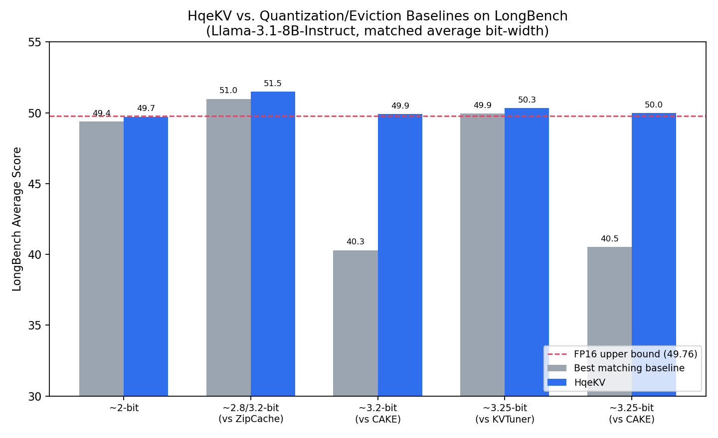
The most dramatic gap is against CAKE (the eviction-only baseline): at matched budget, HqeKV improves the average score from 40.30 to 49.91 (3.2-bit) and from 40.53 to 49.98 (3.25-bit) — roughly a 24% relative improvement, and CAKE’s per-task breakdown (Single-Document QA: 21.44 → 47.38; Multi-Document QA: 17.28 → 40.93) shows the eviction-only baseline suffering catastrophically on exactly the tasks (long single/multi-document QA) where losing entire tokens’ worth of context is most damaging. This is the paper’s strongest piece of evidence that pure eviction is leaving a lot on the table relative to a hybrid approach — a token that gets fully evicted can never contribute to the answer even if the model needed it, whereas a heavily-quantized token can still contribute partial information.

Against the quantization-only baselines (KIVI, OTT, ZipCache, KVTuner) the margins are real but far more modest — for example at 2-bit, KIVI-2 (48.96) and OTT-2 (49.43) versus HqeKV-2 (49.71); at 3.2-bit, ZipCache-3.2 (50.98) versus HqeKV-2.8 (51.26) and HqeKV-3.2 (51.49). These are single-digit-percentage-point gains, not the dramatic eviction-comparison gap. This distinction matters for interpreting the paper’s claims: HqeKV’s advantage over quantization-only competitors is a genuine but incremental refinement (better importance ranking, better bit-width-adaptive strategy selection), while its advantage over eviction-only competitors is closer to a structural win (hybrid compression avoids a failure mode eviction cannot avoid at all). A reader should not come away thinking HqeKV “beats everything by a similar large margin” — the size of the win is very baseline-dependent.

5.2 Reasoning-task transfer (AIME-2025)

On Qwen3-8B with AIME-2025, HqeKV-2 reaches 0.20 accuracy versus KIVI-2’s 0.17 — a real but numerically small gap (3 percentage points on 30 problems, i.e., roughly 1 additional problem solved correctly). This is a useful data point that the method’s benefits are not purely a LongBench artifact, but with only 30 problems in AIME-2025 the statistical power here is limited; a difference of one problem could plausibly be noise rather than signal, and the paper does not report variance across multiple seeds/sampling runs for this specific comparison.

5.3 Memory efficiency and scalability

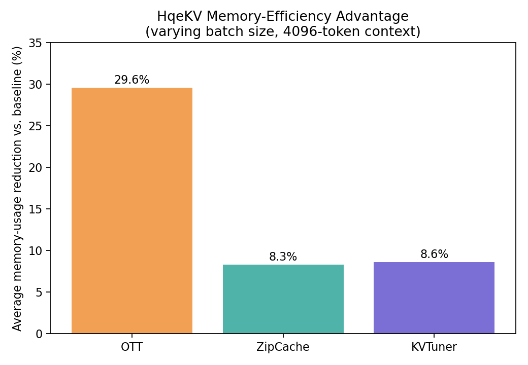
HqeKV reduces memory usage by 29.6% vs. OTT, 8.3% vs. ZipCache, and 8.6% vs. KVTuner on average, and enables the largest achievable batch size in most configurations tested. The paper attributes this to implementation-level factors distinct from the compression algorithm itself: OTT’s per-token 1-norm bookkeeping and outlier-pool overhead, ZipCache’s 10%-token sampling overhead for its attention-weight estimate, and KVTuner’s failure to bit-pack quantized values (leaving unused bits inside byte/word boundaries) versus HqeKV’s use of a custom Triton kernel that densely packs mixed-precision values. This is a legitimate and often-overlooked point: a compression scheme on paper and a compression implementation in a running system can have very different real memory footprints, and the comparison here is at least partly about engineering quality rather than purely about the statistical compression ratio. It would strengthen the paper to separate “algorithmic compression ratio achieved” from “wall-clock/actual-memory efficiency of implementation,” since these are conflated in the reported percentages.

5.4 Ablation: joint metric and search iteration count

The appendix reports (not fully reproduced here) that increasing TPE search iterations from 200 to 300 yields only marginal changes in the resulting precision-ratio allocation (e.g., 4-bit/2-bit/1-bit/eviction ratios of 0.64/0.31/0.04/0.02 at 200 iterations versus 0.65/0.28/0.06/0.02 at 300), suggesting the search converges reasonably quickly and 200 iterations is not leaving significant performance on the table — a useful, if modest, robustness check on the optimizer’s compute budget.

6. Limitations & boundary conditions

The paper’s own Limitations section is refreshingly candid for a venue that often buries limitations in a single throwaway sentence, and is worth quoting close to verbatim before I add my own observations: the offline TPE search for precision ratios is agnostic to user-level or task-level heterogeneity (one global ratio allocation regardless of the downstream task or user), normalized quantization still incurs meaningful conversion loss at 1-bit despite being the better of the two strategies there, the fixed re-quantization interval $T$ is empirically tuned rather than adaptively determined and could be sensitive to context length, and multi-modal architectures (vision-language models with image/video tokens in context) are explicitly flagged as unexplored.

Beyond what the authors state, I’d add:

• Single-GPU, single-vendor evaluation. All experiments run on one RTX A6000. There’s no evidence of how the custom Triton kernel’s memory-packing advantage behaves on different GPU architectures (e.g., H100 with different memory bandwidth/compute ratios), or whether the reported throughput/memory gains hold at data-center batch sizes far beyond what a single 48GB GPU can host.
• Calibration-set generalization is asserted, not stress-tested. WikiText-2 is disjoint from the test benchmarks, which is methodologically correct, but WikiText-2 is a fairly narrow, English-Wikipedia-style text distribution. Whether a precision-ratio allocation calibrated on WikiText-2 transfers well to, say, code-heavy contexts, non-English text, or highly repetitive agentic tool-call traces is untested — and the paper’s own Code Completion column in Table 4 (56.59 → 58.17 FP16-to-HqeKV-2 gap direction, going the wrong way relative to some quantization baselines in places) hints that task-distribution mismatch between calibration and deployment could matter more than the paper’s framing suggests.
• Two model families is a thin generalization base for a method whose core mechanism (the range-error correlation) is claimed to be a general property of Transformer KV caches. Llama-3.1-8B and Qwen3-8B are architecturally similar (both dense decoder-only Transformers with grouped-query attention). Nothing here tests whether the range-quantization-error relationship, or the specific uniform/normalized crossover point, holds for architecturally different families — Mixture-of-Experts models with per-expert KV statistics, models using different positional encodings, or much larger models (70B+) where activation dynamic range characteristics can differ substantially.
• No latency/throughput end-to-end numbers alongside the memory numbers. The paper reports memory reduction and maximum achievable batch size, both important, but does not report end-to-end decode throughput (tokens/sec) under the compression scheme including the overhead of the TPE-search-derived allocation logic, the periodic re-quantization pass, and the joint-metric bookkeeping (tracking a running attention window and value range per cached chunk). For a compression method whose main selling point over eviction is “quality without giving up throughput,” a direct throughput comparison against the fastest baseline would have been a natural and telling addition.

7. Critical analysis

Weaknesses and flaws specific to this paper. The chunk-based averaging of importance (Section 3.3) is a real information-loss source that the paper does not quantify directly — there’s no ablation showing how sensitive final quality is to the chunk size $G=32$, despite $G$ being a hand-set hyperparameter that directly trades off search tractability against ranking granularity. Similarly, the multiplicative joint K-V metric (Section 3.2) is motivated purely by a structural reading of Equation (1) rather than validated against alternative combination rules (weighted sum, max, learned combination), which is a missed opportunity given how central this metric is to the whole system’s decision quality.

Limitations the authors understate or omit. The “never upgrade precision during decoding” policy (Section 3.5) is empirically justified on a single DuReader question with a specific mixed-quantization ratio configuration; generalizing “only 1.18-3.39% of tokens would benefit from an upgrade” to all deployment scenarios, especially long-horizon agentic or retrieval-heavy workloads with non-monotonic relevance patterns, is a stronger claim than the evidence supports, and the Limitations section’s mention of “sensitivity…especially in longer-context scenarios” for the re-quantization interval $T$ gestures at this concern without actually testing it. The paper also does not discuss what happens when the offline-calibrated precision-ratio allocation is wrong for a given deployment — is there a fallback, a way to detect drift, or is the system simply silently worse with no signal to the operator?

Concrete, specific improvement suggestions. First, run an ablation directly varying chunk size $G \in \{8, 16, 32, 64\}$ and reporting both quality and TPE search wall-clock time, so practitioners can make an informed tractability/accuracy trade-off rather than inheriting the paper’s single hand-picked value. Second, replace the single DuReader-question upgrade-transition statistic with a broader study across a stratified sample of LongBench task types (especially the synthetic/needle-style tasks, which are precisely the adversarial case for “never restore” eviction) to give the never-upgrade decoding policy an empirical foundation proportional to how load-bearing it is for the system’s efficiency claims. Third, report end-to-end decode throughput (not just memory/batch-size) against at least the fastest baseline (likely KIVI or OTT), since a practitioner choosing a KV-cache compression method in production cares about the throughput-quality Pareto frontier as much as the memory-quality one, and the current paper only demonstrates the latter directly.

8. Reproducibility & practical notes

Code is publicly released at github.com/skywclouds/HqeKV, which is a meaningful positive relative to a lot of KV-cache-compression papers that release no implementation. The calibration procedure (WikiText-2, 16K tokens, TPE with 200 iterations, explicit hyperparameters $\alpha=2, \beta=4$ for the regularization term) is specified precisely enough in the appendix to be reproducible without guesswork, and the detailed hyperparameter table for every baseline (KIVI group-size 32/residual 128, OTT outlier-token-count 5, ZipCache saliency-ratio 0.6, CAKE window-size 32 with $\tau_1=1.6, \tau_2=0.4$, KVTuner group-size 32/residual 128/avg-bitwidth 3.25) is a genuinely useful contribution for anyone trying to reproduce the comparison table rather than just the proposed method — this level of baseline-configuration transparency is more thorough than many papers in this space bother with. For anyone wanting to actually deploy this: budget for an offline calibration pass per deployment target average bit-width (the search needs to be re-run for each $B_{avg}$ operating point you want to support), and expect to write or adapt a Triton kernel for the dense mixed-precision packing described in Section 5.3’s memory-efficiency discussion, since a naive PyTorch implementation storing five different precision tiers separately would likely erase much of the reported memory advantage.

9. Where this fits in the broader KV-cache compression landscape

Zooming out from HqeKV’s specific mechanisms, it’s worth situating this paper against the trajectory the field has taken since H2O and StreamingLLM first popularized eviction, and KIVI/KVQuant popularized quantization, as competing solutions to the same memory bottleneck. The first generation of methods (2023-2024) largely treated the choice between quantization and eviction as a philosophical commitment — a paper was either an eviction paper or a quantization paper, rarely both, and the comparisons between the two families were mostly indirect (different benchmarks, different bit-width/eviction-ratio conventions, making apples-to-apples memory-matched comparison hard). A second generation (2025, exemplified by ZipCache, KVTuner, CAKE) pushed each family to its own internal limit: mixed-precision quantization got progressively finer-grained (from single-precision to two-tier to layer-sensitive allocation), and eviction got progressively smarter about where in the model to evict from (layer-aware, head-aware policies) rather than just which tokens. HqeKV, together with the two prior hybrid attempts it explicitly positions against (MiniKV, EvicPress), represents an emerging third wave that treats the quantization/eviction boundary itself as the object to be optimized, rather than treating either family as fixed.

The useful generalizable lesson from this paper, independent of whether HqeKV specifically becomes the dominant method, is methodological: whenever a compression (or more broadly, resource-allocation) system offers a genuinely graded scale of actions from “keep everything” to “discard entirely,” the boundary-placement problem deserves the same rigor as the actions themselves. A lot of related-work discussion in this space focuses on how to quantize or how to score importance, and treats the ratio allocation between tiers as an afterthought (manual tuning, fixed thresholds). HqeKV’s TPE-based search, whatever its limitations (Section 6-7), is a concrete existence proof that this boundary-placement sub-problem is itself worth automating and can yield measurable gains, particularly against eviction-only baselines where the all-or-nothing nature of a discarded token leaves the most headroom on the table. Whether TPE specifically remains the right search algorithm as action spaces grow beyond five options (imagine a future system with per-layer, per-head, or per-modality precision tiers) is an open question the paper does not need to answer, but that its framing invites.

References

1. Wang, He, et al. “HqeKV: Towards Hybrid Quantization and Eviction for KV Cache in Long-Context LLM Inference.” Findings of ACL 2026.
2. Zhang, Zhenyu, et al. “H2O: Heavy-Hitter Oracle for Efficient Generative Inference of Large Language Models.” NeurIPS 2023.
3. Liu, Zirui, et al. “KIVI: A Tuning-Free Asymmetric 2bit Quantization for KV Cache.” ICML 2024.
4. Qin, Ziran, et al. “CAKE: Cascading and Adaptive KV Cache Eviction with Layer Preferences.” ICLR 2025.
5. Li, Xing, et al. “KVTuner: Sensitivity-Aware Layer-Wise Mixed-Precision KV Cache Quantization.” ICML 2025.
6. Bergstra, James, et al. “Algorithms for Hyper-Parameter Optimization.” NeurIPS 2011.

---

Review written on 2026-08-26.