Best-Practice Critic Optimization: Making a Learned Critic Beat Group Sampling in LLM RL

Review date: 2026-08-25 Author: Zhongzhu Zhou Paper reviewed: How to Train a Critic Stably and Efficiently Paper authors: Penghui Qi, Xiangxin Zhou, Wee Sun Lee (National University of Singapore; Tencent Hunyuan) arXiv: 2608.23566 Venue/Status: Preprint (cs.LG), August 2026

1. The question this paper actually asks

Reinforcement learning for LLM reasoning has, over the last two years, converged almost entirely on group-based methods: sample several responses per prompt, compare their outcome rewards, and turn that comparison into a per-token training signal. GRPO and its descendants (Dr. GRPO, DAPO, GSPO) all live in this family, and the appeal is obvious — you never have to train a second neural network, and the “baseline” for each response falls straight out of a Monte Carlo group average. The historical alternative, PPO with a learned value function (a critic), fell out of favor for a concrete reason: in practice, critic-based LLM training is fragile. Runs collapse, hyperparameters need per-task retuning, and nobody could point to a small, clearly-stated recipe that reliably worked.

This paper asks a sharper question than “is PPO better or worse than GRPO in general?” It asks: is critic-based RL for LLMs inherently unstable, or is instability an artifact of a handful of specific, fixable implementation choices that most codebases happen to share? The authors’ answer is the latter, and they prove it constructively. They start from a deliberately minimal but revealing failure mode — a “sanity test” where a 1.5B model is fine-tuned on a small set of problems it can already solve, so failing to reach near-100% training reward cannot be blamed on task difficulty or model capacity, only on the optimization recipe. By changing one component at a time and watching the sanity test succeed or fail, they isolate exactly which choices break critic training and which ones fix it. The result, Best-Practice Critic Optimization (BPCO), is not a new algorithm in the sense of a new loss function; it is a specific, empirically justified configuration of existing pieces — DPPO clipping, a bounded value head, an unbiased Monte Carlo critic target, unnormalized advantages, and length-adaptive GAE — plus one genuinely new idea: since the critic is thrown away after training, it can be given information the policy is never allowed to see (a reference answer, an official solution, a grading rubric), and this “privileged” critic input can be used without ever changing what the policy itself observes.

Why should you care if you are not personally debugging a PPO run today? Because the paper’s finding has a structural implication for the field: if a properly configured critic can match GRPO’s sample efficiency while using one rollout per prompt instead of eight or sixteen, then a large chunk of the compute currently spent on “extra samples to get a group baseline” is a workaround for an implementation bug, not a fundamental requirement of critic-free RL. That is a bigger claim than it sounds, and it is worth working through carefully — both the mechanism behind each fix and where the evidence for it does and does not stretch.

This review is organized in three passes. First, prerequisites: what PPO, GAE, and group-based advantage estimation actually compute, since BPCO’s fixes only make sense against this background. Second, the controlled study itself, walking through each of the six components one at a time with the derivation, the failure mode it targets, and the pseudocode. Third, the broader evaluation at scale (larger datasets, 30B-A3B MoE models, rubric-based rewards), followed by an independent critical assessment.

2. Prerequisites

2.1 The credit assignment problem in LLM RL

A language model policy $\pi_\theta$ generates a response $y = (y_1, \dots, y_T)$ token by token, conditioned on a prompt $x$. At each decoding step $t$, the “state” is the prefix $s_t = (x, y_{<t})$, the “action” is the next token $y_t$, and reward is typically sparse and terminal: the whole completed response $y$ gets one scalar reward $R(x, y)$ (say, 1 if a math answer is correct, 0 otherwise), and every intermediate step gets reward 0. This is the outcome-reward setting that both group-based and critic-based methods in this paper target — nobody is claiming per-token reward models here.

The central technical problem is credit assignment: which tokens in a long response should get credit (positive advantage) or blame (negative advantage) for the final 0/1 outcome? Two token-level signals are equally consistent with a single terminal reward — you cannot tell from one rollout alone whether token 47 or token 312 was the pivotal decision. There are exactly two general strategies for estimating a useful per-token advantage without extra reward annotation:

1. Group-relative comparison — sample several responses to the same prompt, and use the differences in their final rewards as the training signal. If a prompt’s group scores mostly 1s and one 0, that 0-response’s tokens all get pushed down.
2. Value function bootstrapping — train a separate model $V_\phi(s_t)$ that predicts the expected future reward from a given prefix, and use the change in this prediction from one step to the next as a token-level advantage signal. Only one rollout per prompt is needed, since the “baseline” comes from the value function, not from other rollouts.

Both strategies are approximations to the same theoretical quantity, the advantage function $A^\pi(s_t, a_t) = Q^\pi(s_t, a_t) - V^\pi(s_t)$, which measures how much better an action is than the policy’s average behavior from that state. Group-based methods approximate this without ever fitting $V^\pi$; critic-based methods fit $V^\pi$ directly. This paper’s contribution lives entirely within the second family: it does not propose a new group-based estimator, it asks how to make the second family actually work.

2.2 Proximal Policy Optimization (PPO), precisely

Given a prompt $x$, let $\mu$ be the “behavior policy” that generated the rollouts used for the current update (in most implementations, $\mu = \pi_{\theta_{\text{old}}}$, the policy snapshot before this gradient step). Define the sampled-token probability ratio at position $t$:

$$\rho_t(\theta) = \frac{\pi_\theta(y_t \mid s_t)}{\mu(y_t \mid s_t)}.$$

Given an advantage estimate $\hat{A}_t$, PPO’s clipped surrogate objective is

$$L_{\mathrm{PPO}}(\theta) = \mathbb{E}_t\Big[\min\big(\rho_t(\theta)\hat{A}_t,\ \mathrm{clip}(\rho_t(\theta), 1-\epsilon, 1+\epsilon)\hat{A}_t\big)\Big]. \tag{1}$$

Intuition: if $\hat{A}_t > 0$ (this token was good), the objective wants to increase $\rho_t$, but the clip caps the reward for doing so once $\rho_t$ exceeds $1+\epsilon$ — the “min” then throws away the gradient beyond that point, so the update stops pushing once the policy has already moved far enough. Symmetrically for $\hat{A}_t < 0$. This creates a trust region: no single minibatch update can move any one token’s probability arbitrarily far in one step, which is the mechanism PPO relies on for stability.

Why this specific clipping form causes trouble at LLM scale. The clip bound $[1-\epsilon, 1+\epsilon]$ is a ratio bound, not an absolute-probability bound. Consider two tokens: one where $\mu(y_t\mid s_t) = 0.9$ and one where $\mu(y_t\mid s_t) = 0.001$. A ratio of $\rho_t = 1.2$ (right at a typical $\epsilon=0.2$ boundary) corresponds to an absolute probability change of $0.9 \to 1.08$ (clipped, since probabilities cannot exceed 1, so effectively a change of $\sim 0.1$) for the first token, but $0.001 \to 0.0012$ for the second — a change 100x smaller in absolute terms. In a vocabulary of 100k+ tokens, most sampled tokens have low probability, so the ratio-based clip systematically permits large absolute swings for common/high-probability tokens while nearly freezing rare/low-probability tokens. This asymmetry is exactly what Divergence Proximal Policy Optimization (DPPO), introduced in a companion paper by the same group, targets.

2.3 Divergence Proximal Policy Optimization (DPPO)

DPPO keeps PPO’s clipped-objective form but replaces the ratio bound with a bound in terms of the sampled token’s probability change. The binary total-variation variant used in this paper is:

$$L_{\mathrm{DPPO}}(\theta) = \mathbb{E}_t\left[\min\left(\rho_t(\theta)\hat{A}_t,\ \mathrm{clip}\left(\rho_t(\theta),\ 1 - \frac{\epsilon}{\mu(y_t\mid s_t)},\ 1 + \frac{\epsilon}{\mu(y_t\mid s_t)}\right)\hat{A}_t\right)\right]. \tag{2}$$

Derivation of why this is equivalent to an absolute-probability constraint. Write the clip boundary as $\rho_t \le 1 + \epsilon/\mu(y_t\mid s_t)$. Multiplying both sides by $\mu(y_t\mid s_t)$ (positive, so the inequality direction is preserved):

$$\rho_t(\theta)\, \mu(y_t\mid s_t) \le \mu(y_t\mid s_t) + \epsilon.$$

But $\rho_t(\theta)\,\mu(y_t\mid s_t) = \pi_\theta(y_t \mid s_t)$ by definition of $\rho_t$. So the upper clip boundary is exactly $\pi_\theta(y_t\mid s_t) \le \mu(y_t\mid s_t) + \epsilon$, and symmetrically the lower boundary gives $\pi_\theta(y_t\mid s_t) \ge \mu(y_t\mid s_t) - \epsilon$. Combining: $|\pi_\theta(y_t\mid s_t) - \mu(y_t\mid s_t)| \le \epsilon$ — an absolute probability-shift constraint, identical in nature for a token with $\mu=0.9$ and a token with $\mu=0.001$. This is the “common absolute-probability threshold rather than a common ratio threshold” the paper describes. The obvious alternative the authors could have used instead — just shrinking $\epsilon$ uniformly to control the worst-case low-probability-token blowup — would over-constrain high-probability tokens, since a smaller $\epsilon$ caps everyone’s absolute movement at the same (small) value; DPPO’s per-token rescaling by $1/\mu(y_t\mid s_t)$ lets high-probability tokens move by a larger ratio (since their absolute probability has more “room” below 1) while still capping everyone’s absolute movement at $\epsilon$.

The paper’s own sanity test (Section 3.1, discussed below) shows this is not a cosmetic difference: replacing PPO with DPPO is the single change that turns a collapsing training run into a stable one, before any of the critic-specific fixes are applied. This establishes DPPO as the fixed foundation on top of which the remaining five BPCO components are layered.

A concrete numeric illustration. Take $\epsilon = 0.2$, the common PPO default. For a high-probability token with $\mu(y_t\mid s_t) = 0.9$, PPO’s ratio clip permits $\rho_t \in [0.8, 1.2]$, i.e. $\pi_\theta(y_t\mid s_t) \in [0.72, 1.08]$ (clipped at 1) — an absolute swing of up to $0.1$. For a low-probability token with $\mu(y_t\mid s_t) = 0.001$, the same ratio clip permits $\pi_\theta(y_t\mid s_t) \in [0.0008, 0.0012]$ — an absolute swing of only $0.0002$, five hundred times smaller. Under DPPO with the same nominal $\epsilon = 0.2$ scaled per-token as $\epsilon/\mu(y_t\mid s_t)$, the high-probability token’s effective ratio bound becomes $1 \pm 0.2/0.9 \approx 1\pm 0.222$ (barely different from PPO, since $\mu$ is already close to 1), while the low-probability token’s effective ratio bound becomes $1 \pm 0.2/0.001 = 1\pm 200$ — an enormous ratio range, but one that, multiplied back through by $\mu = 0.001$, still corresponds to exactly the same $\pm 0.2$ absolute-probability window as the high-probability token. This numeric asymmetry is precisely why a large-vocabulary LLM, where the overwhelming majority of sampled tokens sit at low absolute probability, sees such different practical clipping behavior between PPO and DPPO.

2.4 Generalized Advantage Estimation (GAE) and the critic target, derived

For rollouts generated by behavior policy $\mu$, define the true value function $V^\mu(s_t) = \mathbb{E}_\mu[R(x,y) \mid s_t]$ — the expected final reward given everything generated so far. A critic $V_\phi(s_t)$ is a neural network trained to approximate this quantity. Let $\phi_{\text{old}}$ denote a frozen snapshot of the critic parameters used only to construct targets (this decoupling from the currently-updating $\phi$ is standard and prevents a moving target during a single update).

Step 1 — the TD residual. Define the one-step temporal-difference error at each position:

$$\delta_t = r_t + \gamma V_{\phi_{\text{old}}}(s_{t+1}) - V_{\phi_{\text{old}}}(s_t). \tag{3}$$

Intuition: $r_t + \gamma V_{\phi_{\text{old}}}(s_{t+1})$ is a one-step-lookahead re-estimate of $V(s_t)$ (bootstrap using the next state’s critic value plus the reward actually observed at this step), and $\delta_t$ is how much that re-estimate disagrees with the critic’s own current prediction at $s_t$. If the critic were perfect, $\delta_t = 0$ everywhere in expectation.

Step 2 — the exponentially-weighted sum (GAE). Rather than using $\delta_t$ alone (high variance if $\gamma$ close to 1 over long horizons, since it’s a raw one-step estimate) or the full Monte Carlo return alone (also high variance, since it must accumulate every future step’s actual randomness), GAE interpolates between the two with a geometric weighting:

$$\hat{A}_t^{\mathrm{GAE}(\lambda)} = \sum_{l=0}^{T-t} (\gamma\lambda)^l\, \delta_{t+l}. \tag{4}$$

Here $r_t = 0$ for $t < T$ (outcome-only reward), $r_T = R(x,y)$, and $V_{\phi_{\text{old}}}(s_{T+1}) = 0$ (no reward beyond the end of the response). The discount $\gamma$ and the trace-decay parameter $\lambda \in [0,1]$ jointly control the bias-variance tradeoff: $\lambda = 0$ reduces to the raw one-step TD residual (low variance, high bias from critic error); $\lambda = 1$ makes the sum telescope — expand the geometric sum and note the $V_{\phi_{\text{old}}}$ terms cancel pairwise except at the boundary — to $R(x,y) - V_{\phi_{\text{old}}}(s_t)$, the pure Monte Carlo advantage with zero bootstrapping (unbiased with respect to $V^\mu$, but higher variance since it inherits the full randomness of the sampled continuation).

Step 3 — the naive critic target. The textbook approach constructs the regression target for the critic itself from the same $\hat{A}_t^{\mathrm{GAE}(\lambda)}$ used for the policy:

$$\hat{V}_t(\lambda) = \hat{A}_t^{\mathrm{GAE}(\lambda)} + V_{\phi_{\text{old}}}(s_t), \qquad \mathcal{L}_V(\phi) = \mathbb{E}_t\Big[\big(V_\phi(s_t) - \hat{V}_t(\lambda)\big)^2\Big]. \tag{5, 6}$$

Why this naive coupling is a design flaw, not just a minor inefficiency. Substitute the definition of $\hat{A}_t^{\mathrm{GAE}(\lambda)}$ back into Equation 5: whenever $\lambda < 1$, $\hat{V}_t(\lambda)$ is a weighted combination that itself contains $V_{\phi_{\text{old}}}$ terms (through the $\delta_{t+l}$ residuals for $l>0$). This means the critic is partly being trained to reproduce its own previous predictions — a self-referential target. A critic can achieve a target that looks well-fit (high “explained variance” against $\hat{V}_t(\lambda)$) simply by staying close to its own last iterate, regardless of whether that iterate is close to the true observed outcome $R(x,y)$. This is exactly the failure mode the paper isolates in Section 3.3 (Step 3 below): explained variance against the bootstrapped target shoots to near 1 while the policy is visibly unstable, because the metric is measuring self-consistency, not accuracy.

2.5 Group-based methods (GRPO / Dr. GRPO) as the comparison baseline

Group-based methods sidestep the critic entirely by sampling $G$ responses $\{y^{(i)}\}_{i=1}^G$ for the same prompt $x$. Let $R_i = R(x, y^{(i)})$, and let $\mu_R, \sigma_R$ be the empirical mean and standard deviation across the group. GRPO assigns every token in response $i$ the same advantage:

$$\hat{A}_{t,i}^{\mathrm{GRPO}} = \frac{R_i - \mu_R}{\sigma_R}. \tag{7}$$

Dr. GRPO removes the $\sigma_R$ normalization (which the DAPO/Dr. GRPO literature has separately shown reweights prompts by their within-group reward variance in a way that is not obviously desirable — prompts that happen to produce a very tight spread of rewards get amplified gradients relative to prompts with a wide spread, even if both prompts are equally informative):

$$\hat{A}_{t,i}^{\mathrm{Dr.GRPO}} = R_i - \mu_R. \tag{8}$$

This is the baseline BPCO is measured against in Section 4. The key structural difference to keep in mind throughout the rest of this review: group-based methods need $G$ rollouts of the same prompt to construct one advantage estimate (BPCO’s baseline experiments use $G=16$); critic-based methods, once trained, need only 1.

3. Building BPCO: the controlled sanity-test study

3.1 The experimental design that makes the paper convincing

Before getting into each fix, it’s worth appreciating the experimental design choice that gives this paper its evidentiary weight. The authors fine-tune DeepSeek-R1-Distill-Qwen-1.5B on 1,460 math problems that the initial model can already solve. A correctly configured RL recipe should therefore drive training reward to nearly 100% — if it does not, the failure is attributable to the optimization recipe, not to task difficulty, insufficient model capacity, or a noisy reward signal. This is the same logic as a unit test: the outcome is known in advance, so any deviation is diagnostic. Each run uses 1,024 trajectories per iteration, minibatch size 256 (four optimizer minibatches per iteration), policy learning rate $10^{-6}$, critic learning rate $10^{-5}$, and runs for 1,500 iterations. A held-out metric, AIME 2025 avg@32 (mean accuracy over 32 samples per problem on a genuinely hard benchmark), is monitored throughout to catch overfitting to the small training set — a recipe that fits the 1,460 problems perfectly but destroys general reasoning ability would also be a failure, just a different kind.

The authors change one component at a time, starting from vanilla PPO with standard GAE and $\lambda=1$, and each subsequent step retains all prior changes. This ablation-in-sequence design is what lets the paper make causal claims (“removing X specifically fixes failure mode Y”) rather than just correlational ones (“the final recipe works better than the initial one”).

3.2 Step 1 — replacing PPO with DPPO

What breaks and why. With plain PPO ($\lambda=1$), training reward rises initially, then collapses to near zero after roughly iteration 400 (Figure 1, blue curve). Swapping in the DPPO objective (Equation 2) with everything else unchanged produces a stable climb to near-1.0 training reward and a corresponding steady rise in AIME 2025 avg@32 (green curve). This confirms Section 2.3’s mechanism directly: at $\lambda=1$ there is no bootstrapped critic error feeding into the advantage (the GAE sum telescopes to the pure Monte Carlo advantage), so the only remaining difference between the collapsing PPO run and the stable DPPO run is the clipping rule itself — strong evidence that ratio-based clipping’s uneven treatment of low- vs. high-probability tokens is sufficient on its own to destabilize training, even with an otherwise-unbiased advantage signal.

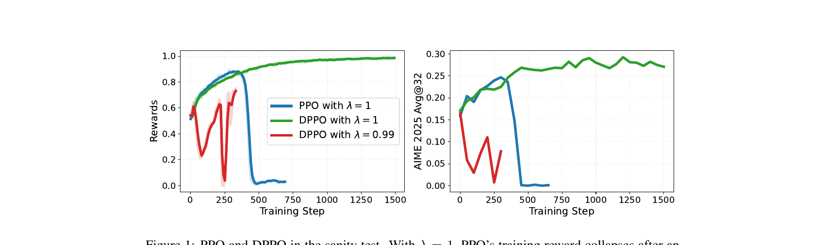
The stress test that sets up the rest of the paper. The authors then reduce $\lambda$ to 0.99 under DPPO and observe instability returns (red curve in Figure 1) — DPPO alone is not sufficient once the advantage estimate contains any bootstrapped critic predictions, since critic approximation error $V_\phi \ne V^\mu$ now biases the advantage relative to the unbiased $\lambda=1$ estimator. Rather than treating this as a reason to always use $\lambda=1$ (which would defeat the variance-reduction purpose of GAE), the authors deliberately keep $\lambda=0.99$ as a stress test for the remaining steps: the rest of BPCO’s design is explicitly aimed at making training robust to bootstrapped critic error, not at avoiding bootstrapping altogether. This is an important design-philosophy point — a recipe that only works at $\lambda=1$ would sacrifice all of GAE’s variance-reduction benefit, which matters more as horizons get longer.

3.3 Step 2 — bounding the critic’s value predictions to the reward range

The problem. A standard critic uses a linear head: $V_\phi(s_t) = w^\top h(s_t) + b$ for some hidden representation $h$. Nothing constrains this output to the known range of the return — for the sanity test’s binary $\{0,1\}$ rewards, a linear head can and does output values like $8$ or $-8$ (Figure 2, right panel, blue curve), which is provably impossible for the expectation of a Bernoulli-like return. These extreme predictions destabilize the training reward and AIME score (Figure 2, left/middle, blue curves) even though DPPO alone (from Step 1) was stable at $\lambda=1$ — the instability re-emerges here because Step 2’s stress test uses $\lambda=0.99$, reintroducing critic error into the advantage, and now that error can be arbitrarily large in magnitude because nothing bounds it.

The fix, derived. Let $[R_{\min}, R_{\max}]$ be the known reward range ($[0,1]$ for binary rewards) and $z_\phi(s_t) \in \mathbb{R}$ be the raw linear head output. Since $V^\mu(s_t) = \mathbb{E}_\mu[R(x,y)\mid s_t]$ is an expectation of a bounded random variable, it must itself lie in $[R_{\min}, R_{\max}]$ — this is not a modeling choice, it is a mathematical fact about expectations of bounded variables that the standard linear head simply ignores. The paper enforces it with a scaled arctangent squashing function:

$$V_\phi(s_t) = R_{\min} + (R_{\max} - R_{\min})\left(\frac{1}{2} + \frac{1}{\pi}\arctan\big(z_\phi(s_t)\big)\right). \tag{9}$$

Why arctangent and not, say, sigmoid? Both map $\mathbb{R}$ to a bounded open interval and are algebraically similar in shape. The paper does not explicitly justify the choice over sigmoid, and this is worth flagging as a design choice without a stated rationale (see Section 6 below) — empirically the two would very likely behave near-identically for this purpose, since both are smooth, monotonic bijections onto $(R_{\min}, R_{\max})$ with similar saturation behavior; the choice is likely a matter of the codebase’s existing convention rather than a deliberate result of comparison. The important property both share, and what actually matters: (a) the map is monotonic, so gradient signal is preserved (no flat regions except in the far tails where saturation legitimately reflects extreme confidence); (b) every finite input maps to the open interval, never touching the boundary exactly, so gradients from a squared-error loss are always well-defined; (c) the asymptotic saturation at $R_{\min}$/$R_{\max}$ means very confident predictions produce very small gradients near the boundary, which is generally desirable (you do not want a huge gradient pushing a nearly-certain prediction over the edge into an impossible value).

With this fix, Figure 2 shows the bounded-value critic (green) tracks a stable, monotonically improving training reward and AIME curve, essentially matching the earlier $\lambda=1$ stability from Step 1, while the value predictions themselves (right panel, green) stay pinned inside $[0,1]$.

Algorithm 1 — bounded critic head (pseudocode).

Algorithm 1: Reward-Range-Bounded Value Head
Input: hidden representation h(s_t), reward bounds R_min, R_max, linear params (w, b)
1: z <- w^T h(s_t) + b                     # raw unbounded scalar
2: u <- 0.5 + (1/pi) * arctan(z)           # squash to open interval (0, 1)
3: V_phi(s_t) <- R_min + (R_max - R_min) * u
4: return V_phi(s_t)

3.4 Step 3 — using an unbiased Monte Carlo value target

Diagnosing the self-referential target. As derived in Section 2.4, the naive critic target $\hat{V}_t(\lambda)$ contains $V_{\phi_{\text{old}}}$ whenever $\lambda < 1$. The paper tracks an explained variance diagnostic:

$$\mathrm{EV}(V_\phi, \hat{V}) = 1 - \frac{\mathrm{Var}(\hat{V}_t - V_\phi(s_t))}{\mathrm{Var}(\hat{V}_t)}. \tag{10}$$

Ordinarily, $\mathrm{EV} \to 1$ signals a good fit. But Figure 3 (right panel) shows explained variance against the bootstrapped target $\hat{V}_t(0.99)$ rapidly approaching 1 while training reward and AIME (left/middle) remain unstable — direct empirical confirmation of the self-referential-target failure mode: the critic is fitting a moving target that partly consists of its own recent predictions, so a high EV score here means “consistent with itself,” not “accurate against the true outcome.”

The fix — decoupled GAE, following VC-PPO. Use separate $\lambda$ values for the policy advantage and the critic target: keep $\lambda_\pi = 0.99$ for the policy (retaining variance reduction), but set $\lambda_V = 1$ for the critic’s own regression target. With $\gamma=1$ and outcome-only rewards, substituting $\lambda_V=1$ into the GAE sum makes it telescope exactly as derived in Section 2.4:

$$\hat{V}_t = \hat{A}_t^{\mathrm{GAE}(1)} + V_{\phi_{\text{old}}}(s_t) = R(x,y). \tag{11}$$

This is now literally the observed final outcome — a genuine, unbiased Monte Carlo sample of $V^\mu(s_t)$ for any prefix along a trajectory sampled from $\mu$, with zero dependence on $V_{\phi_{\text{old}}}$. The key insight generalizable beyond this paper: the policy advantage and the critic’s own training target do not have to be computed with the same $\lambda$. Decoupling them lets you keep low-variance bootstrapped advantages for the policy gradient while still training the critic itself against ground truth. After this fix, Figure 3 shows both stable training reward/AIME curves and an EV metric that is now measured against the true outcome and rises to a sensible level (not spuriously near-1).

Why not just always use $\lambda_\pi = 1$ too (avoiding the mismatch altogether)? That is exactly the alternative the authors implicitly test in Step 6 below (Figure 6) — it removes the instability risk but is empirically slower to reach a given reward level, because pure Monte Carlo advantages have higher variance per sample. Decoupling is a way to keep both benefits rather than trading one off against the other.

3.5 Step 4 — removing batch-wise advantage normalization

The transformation and why it seems reasonable. Many PPO implementations normalize advantages within each training batch before the policy update: with batch mean $\bar{A}$ and standard deviation $\sigma_A$,

$$\tilde{A}_t = \frac{\hat{A}_t - \bar{A}}{\sigma_A}. \tag{12}$$

The intuitive appeal is straightforward: this keeps the effective learning rate roughly consistent across training regardless of the raw reward scale, similar to why batch normalization helps supervised training. But the paper argues this is fundamentally wrong for RL near convergence, and the argument is worth spelling out in full.

Why it breaks near-optimal policies. Consider a policy that has nearly converged: true advantages $A_t$ are small in magnitude and have small variance, because there is little room left to improve. A well-behaved training signal should then also shrink — smaller true advantages should produce smaller policy updates, since there is genuinely less to learn. But dividing by $\sigma_A$ actively undoes this: if $\sigma_A \to 0$ (the honest and desirable outcome of a near-converged policy), the normalized advantage $\tilde{A}_t = (\hat{A}_t - \bar{A})/\sigma_A$ rescales pure estimation noise into an update of unit-scale magnitude, regardless of how small the true signal actually is. The policy therefore keeps taking full-sized gradient steps driven almost entirely by sampling noise, exactly when it should be taking near-zero steps. A secondary problem: subtracting $\bar{A}$ can flip the sign of examples whose true advantage is small-but-positive if it happens to fall below the batch mean, actively discouraging behavior that was in fact slightly above average — a corrosive effect on exploration, since it punishes marginally-good actions purely because of where the batch happened to land that step.

Empirical confirmation. Figure 4 (right panel) shows the advantage range under normalization growing over training (reaching magnitudes of 40-60) rather than shrinking as the policy approaches convergence — the opposite of the desired behavior. Without normalization (raw GAE advantages), the range stays small and stable throughout. The middle panel shows normalization also increases overfitting risk on the held-out AIME metric, consistent with the “noise amplification near convergence” mechanism — more aggressive-than-warranted updates late in training push the policy to overfit the training distribution.

The obvious alternative the authors reject, and why. One might keep normalization but clip $\sigma_A$ away from zero (a common fix elsewhere, e.g., in normalizing rewards) — the paper does not test this variant explicitly, which is a gap worth noting, but the sign-flipping problem from subtracting $\bar{A}$ would persist regardless of how $\sigma_A$ is floored, so a $\sigma_A$-floor alone would not fully address the paper’s stated concerns.

3.6 Step 5 — privileged information for the critic

The core observation. Nothing requires the critic’s input to match the policy’s input. The critic exists only during training and is discarded afterward; the policy’s deployment-time behavior is entirely determined by what the policy itself sees. This mirrors centralized training with decentralized execution in multi-agent RL (e.g., a training-time critic in StarCraft II agents that sees the full game state while each unit’s policy sees only local observations) — the training signal can be arbitrarily rich as long as the thing actually being deployed stays within its real input constraints.

Applying this to reward-defining information. Let $q(x)$ denote information that determines how a response to prompt $x$ is scored — a reference answer for a math problem, an official worked solution, or a grading rubric for an open-ended task. Since $q(x)$ is a deterministic function of the prompt $x$ itself, it cannot change the true value function $V^\mu(s_t)$ — the ideal value is already implicitly a function of $x$ through the reward function. What privileged information changes is how easy that value is to approximate with a finite-capacity critic:

$$V_\phi^\mu(s_t, q(x)) \approx \mathbb{E}_\mu[R(x,y;q(x)) \mid s_t, q(x)]. \tag{13}$$

Intuitively: predicting “will this partial derivation lead to the correct answer” is a much easier learning problem if the critic is explicitly shown the correct answer than if it has to infer everything about correctness from the prefix alone. The rollout policy is completely unaffected — it never sees $q(x)$, generates identically to a non-privileged setup, and its deployment-time behavior is unchanged.

Empirical result and an important caveat. Figure 5 shows the reference-answer-conditioned critic achieves both faster training-reward improvement and higher explained variance — direct confirmation that privileged input makes the regression problem easier for the critic. But the AIME 2025 validation curve rises faster and then peaks earlier and declines relative to the non-privileged version — the paper’s own words, “a more informative critic can accelerate both learning and overfitting.” This is the paper’s most important nuance and the authors do not shy away from stating it plainly: privileged information is useful but not uniformly beneficial, and its benefit is contingent on dataset size relative to model capacity (this specific instance uses a small 1,460-problem sanity-test dataset, which is exactly the regime where overfitting risk is highest).

3.7 Step 6 — length-adaptive GAE

The problem with a fixed $\lambda_\pi$. For a token at position $t$ in a response of total length $L=T$, the coefficient on the terminal TD residual (i.e., the term in the GAE sum that actually carries information about the final reward) is proportional to $\lambda_\pi^{T-t}$. For an early token in a long response, $T - t$ is large, so this coefficient is tiny — meaning the early-token advantage is dominated almost entirely by intermediate bootstrapped critic residuals, not by the actual final outcome. If the critic has any systematic bias, that bias dominates the advantage signal for early tokens in long responses specifically, while barely affecting late tokens or short responses. A single fixed $\lambda_\pi$ therefore implicitly treats short and long responses very differently, without that being an intentional design choice.

The fix, derived. Following VAPO and SAO, make $\lambda_\pi$ a function of the response length $L = |y|$:

$$\lambda_\pi(L) = 1 - \frac{1}{\alpha L}, \qquad \alpha > 0. \tag{14}$$

Why this specific functional form. The terminal-residual coefficient for the earliest token becomes $\lambda_\pi(L)^L = \left(1 - \frac{1}{\alpha L}\right)^L$. Take the limit as $L \to \infty$: this is the standard $\left(1 - \frac{c}{n}\right)^n \to e^{-c}$ limit from calculus, with $c = 1/\alpha$ and $n=L$, giving $\left(1-\frac{1}{\alpha L}\right)^L \to \exp(-1/\alpha)$ — a constant independent of $L$. So while a fixed $\lambda_\pi$ gives the terminal reward exponentially vanishing weight as responses get longer, the length-adaptive form in Equation 14 keeps that weight approximately invariant to response length by increasing $\lambda_\pi$ (moving it closer to 1, i.e., less bootstrapping) proportionally as $L$ grows. Short responses get more bootstrapping (lower effective $\lambda$, faster variance reduction since there is less to integrate over anyway); long responses get correspondingly less bootstrapping per unit length, keeping the terminal signal’s influence roughly constant in relative terms across response lengths.

Empirical trade-off (Figure 6). Fixed $\lambda_\pi = 0.99$ fits the training set fastest (left panel) but shows a pronounced decline in AIME avg@32 after an early peak (middle panel) — a textbook overfitting signature, consistent with the “bootstrapped bias dominates” mechanism above compounding over training. Fixed $\lambda_\pi = 1$ (pure Monte Carlo, no bootstrapping at all) avoids the decline entirely but is markedly slower to reach a given reward level. Length-adaptive GAE with $\alpha = 0.4$ threads this needle, retaining most of $\lambda=0.99$‘s early training speed while avoiding its later validation decline — an empirically-tuned middle ground rather than a value derived from first principles (the paper does not report a sweep over $\alpha$ beyond this one value, which is a reproducibility gap worth flagging explicitly).

Algorithm 2 — the assembled BPCO training step (pseudocode).

Algorithm 2: One BPCO Policy+Critic Update
Input: rollouts {(s_t, y_t, r_t)} from behavior policy mu, frozen critic phi_old,
       reward bounds [R_min, R_max], DPPO epsilon, alpha (length-adaptive GAE)
1: for each rollout of length L:
2:     lambda_pi <- 1 - 1/(alpha * L)          # Eq. 14, per-response
3:     lambda_V   <- 1                          # always, decoupled from lambda_pi
4:     for t = T down to 1:                     # backward recursion for GAE
5:         delta_t <- r_t + V_phi_old(s_{t+1}) - V_phi_old(s_t)     # Eq. 3, gamma=1
6:         A_hat_pi[t]  <- delta_t + lambda_pi * A_hat_pi[t+1]       # Eq. 4 w/ lambda_pi
7:         A_hat_V[t]   <- delta_t + lambda_V  * A_hat_V[t+1]        # Eq. 4 w/ lambda_V=1
8:     V_target[t] <- A_hat_V[t] + V_phi_old(s_t)   # Eq. 11, telescopes to R(x,y)
9: # Policy update (no advantage normalization -- Step 4)
10: theta <- theta + grad_theta L_DPPO(theta; {A_hat_pi[t]})   # Eq. 2, raw A_hat_pi
11: # Critic update (bounded value head -- Step 2; unbiased target -- Step 3)
12: phi <- phi - grad_phi  MSE(V_phi(s_t; [privileged q(x) if available]), V_target[t])
13: return theta, phi

Note line 7 uses $\lambda_V = 1$, which via the telescoping argument in Equation 11 simplifies the backward recursion for the critic target to simply propagating the terminal reward backward unchanged — the pseudocode keeps the general recursive form to make the parallel with the policy-advantage computation explicit, since a real implementation can (and the paper’s does) just set V_target[t] = R(x,y) directly for every $t$ once $\lambda_V=1$ is fixed.

4. Broader evaluation

4.1 Scaling to a larger dataset (DeepScaleR, 40.3K problems)

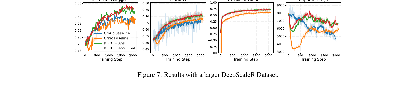
Moving beyond the deliberately tiny sanity-test dataset, the authors fine-tune the same 1.5B model on DeepScaleR (40.3K math problem-answer pairs, official solutions available for ~7.3K of them, max response length 24k tokens). Figure 7 compares four configurations: the Dr. GRPO group baseline ($G=16$), a “critic baseline” that includes decoupled GAE and length-adaptive GAE from Steps 3 and 6 but retains the unbounded value head and batch-wise advantage normalization (i.e., everything except Steps 2 and 4), BPCO+Ans (privileged reference answer), and BPCO+Ans+Sol (privileged reference answer plus official solution where available).

The result: BPCO+Ans and BPCO+Ans+Sol both clearly outperform the critic baseline on AIME 2025 avg@32 (left panel) and match or slightly exceed the group baseline, while the critic baseline visibly lags both. The explained-variance panel is the most diagnostic: BPCO variants maintain consistently higher EV throughout training relative to the critic baseline — direct evidence that Steps 2 and 4 (the only difference between BPCO and this “critic baseline”) specifically improve the critic’s own fit quality, not just downstream policy performance by some indirect mechanism. This matters because it isolates causality: a model could plausibly get better policy scores through some unrelated regularization side-effect of bounding values or removing normalization, but the EV curve shows the critic itself genuinely fits the data better.

4.2 Ablating the two remaining BPCO-specific tricks at this larger scale

Starting from a well-trained BPCO+Ans run, the authors ablate one component at a time in the opposite direction (removing a good component / adding back a bad one), which is a nice methodological symmetry with the sanity-test build-up.

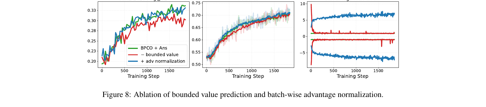
Removing the value bound (Figure 8, ”− bounded value” curve). Reintroducing an unconstrained linear value head slows training-reward improvement and lowers AIME performance relative to the full BPCO+Ans recipe, though the gap is visibly smaller than in the sanity test — the authors attribute this to the larger, more diverse dataset providing enough regularization pressure that the unbounded head does not blow up as catastrophically as in the tiny sanity-test dataset, but the bound still measurably helps.

Adding back advantage normalization (Figure 8, ”+ adv normalization” curve). The advantage range grows over training (right panel, blue) just as in the sanity test, though the effect on downstream reward/AIME performance is smaller and the authors candidly note “training is not fully converged” in this comparison — i.e., they have not run long enough to see whether the growing-advantage pathology would eventually cause the same kind of late-training instability observed in the sanity test. They still recommend removing normalization universally based on the mechanism, even where the empirical gap at this specific training budget is modest.

Privileged information at scale (Figure 9). With ground-truth answers, training is visibly faster and explained variance higher than plain BPCO; with official solutions (available for only 7.3K/40.3K problems, i.e., partial coverage), the improvement is smaller but still present. This is a useful robustness result: privileged information helps even when available for a minority of training examples, suggesting the critic can partially generalize the “how to use extra context” skill to examples where that context is absent, though the paper does not directly test this generalization claim (e.g., by measuring EV specifically on the no-solution subset).

4.3 Scaling to larger MoE models (Qwen3-30B-A3B and Qwen3-30B-A3B-Base)

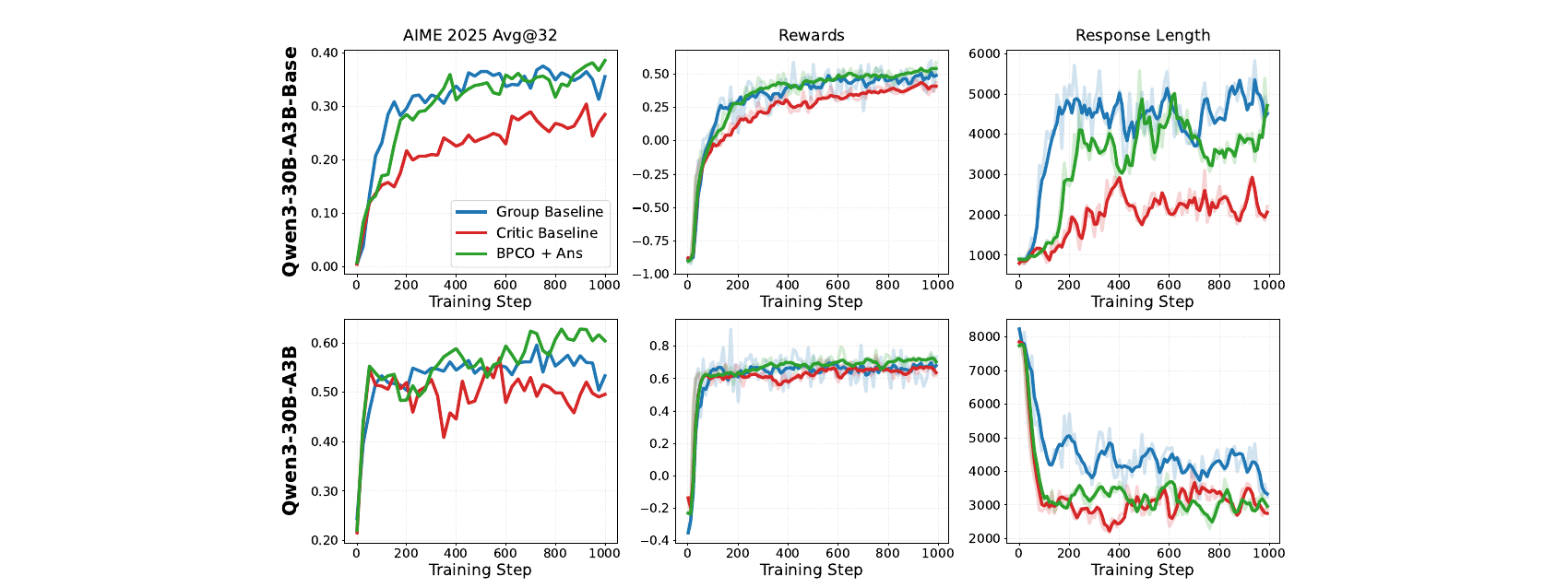
Figure 10 repeats the three-way comparison (group baseline, critic baseline, BPCO+Ans) on two 30B-parameter, 3B-active-parameter mixture-of-experts models using the DAPO-Math-17k dataset. Two results stand out. First, on the base (non-instruction-tuned) model, the critic baseline’s AIME curve visibly stalls and stays well below both BPCO+Ans and the group baseline — a case where the standard critic-based recipe simply fails to keep improving, while BPCO continues to climb. Second, on the instruct-tuned Qwen3-30B-A3B, the paper reports the critic baseline “failed to further improve AIME 2025 after the first 100 training steps, suffering from an unstable optimization,” while BPCO+Ans continues climbing throughout the full 1,000-step run and modestly exceeds the group baseline. This is the paper’s strongest scale-generalization evidence: the sanity-test-derived fixes transfer to a genuinely different model family, size, and architecture (MoE routing introduces its own potential sources of critic-training difficulty that the dense 1.5B sanity test could not have surfaced) and continue to matter.

4.4 Rubric-based rewards (a qualitatively different reward source)

The final experiment moves away from verifiable math rewards entirely: Qwen3-4B-Base is trained as both policy and critic on OpenRubrics, with Qwen3-4B-Instruct-2507 acting as an LLM judge that scores generated responses against per-prompt “golden rubrics” (invisible to the policy, used as privileged critic input). Figure 11 shows both BPCO variants (with and without privileged rubric input) improving faster than the critic baseline and than the group baseline early on, though the group baseline eventually converges to comparable final performance. Interestingly, privileged rubric information brings no validation performance benefit here despite producing higher explained variance — the paper attributes this to the task being “relatively trivial,” i.e., the critic can already approximate the value function well without the rubric, so there is no headroom left for privileged information to close. This is a useful negative result precisely because it delineates where privileged information helps (harder, more ambiguous credit-assignment problems) versus where it does not (easier tasks where the non-privileged critic already fits well).

5. Design choices: a consolidated why/alternative/boundary summary

Design choice	Why it works	Obvious alternative	Where it could fail
DPPO instead of PPO clipping	Bounds absolute probability shift, not ratio, avoiding uneven treatment of low/high-probability tokens	Uniformly shrink PPO’s $\epsilon$	Over-constrains updates for common tokens if $\epsilon$ is set small enough to control rare-token blowup
Arctangent-bounded value head	Guarantees $V_\phi \in [R_{\min}, R_{\max}]$, a mathematical necessity for bounded rewards	Sigmoid squashing (algebraically similar)	Requires a known, fixed reward range; unbounded or heavy-tailed reward models would need re-deriving the bound
Decoupled $\lambda_\pi \ne \lambda_V$	Keeps policy-side variance reduction while removing self-referential critic target	Set both to 1 (pure Monte Carlo everywhere)	Loses GAE’s variance reduction for the policy on long-horizon tasks
Removing batch advantage normalization	Prevents noise amplification as the policy nears convergence; avoids spurious sign flips	Floor $\sigma_A$ away from zero	Does not fix the mean-subtraction sign-flip issue; not tested by the paper
Length-adaptive GAE	Keeps terminal-reward influence roughly length-invariant	Fixed $\lambda_\pi=1$ (no bootstrapping)	Slower training; the specific $\alpha=0.4$ is not shown to transfer beyond the one dataset/model tested
Privileged critic information	Reduces the critic’s approximation burden without changing policy inputs	Give the policy the same information (curriculum-style)	Would change the deployed model’s I/O contract, and increases overfitting risk in small-data regimes

6. Limitations, and where the authors likely understate them

What the authors state explicitly. The paper’s own limitations paragraph is notably candid but brief: evidence is limited to mathematical and rubric-based rewards; BPCO assumes a known reward range; privileged variants require evaluator-side information (a reference answer, solution, or rubric) that may not exist for every task; and critic training adds real compute and memory overhead that the trajectory-matched comparisons in the paper do not fully account for.

What is understated or left implicit:

• The reward-range assumption is stronger than it sounds. Binary $\{0,1\}$ correctness rewards and bounded rubric scores are convenient cases. Many real RLHF pipelines use learned reward models whose output distribution is not naturally bounded (or is bounded only by an arbitrary clip applied post-hoc, which reintroduces exactly the kind of ad-hoc engineering choice this paper otherwise argues against). The paper never demonstrates BPCO with an unbounded or heavy-tailed reward model, which is arguably the single most common reward setup in production RLHF outside of verifiable-math and rubric domains.
• $\alpha=0.4$ for length-adaptive GAE is presented as a settled hyperparameter but is only validated on the 1.5B sanity-test model. The larger-scale experiments (Section 4.1-4.3) do not report whether $\alpha$ was re-tuned for the 30B-A3B models or the longer 24k-token DeepScaleR responses; if it was kept fixed, that is worth stating explicitly, since the derivation in Section 2’s Equation 14 shows the effective discounting behavior of a given $\alpha$ depends on the typical response length distribution, which differs substantially between the sanity-test dataset and DeepScaleR/DAPO-Math-17k.
• The “single rollout per prompt” framing slightly overstates the compute parity claim. BPCO is compared against Dr. GRPO with $G=16$ per prompt “matching the total batch size” — meaning BPCO uses more distinct prompts per batch rather than fewer total rollouts. This is a fair comparison for prompt diversity, but the critic itself requires a full forward+backward pass through a second network of comparable size to the policy at every training step (unless a much smaller critic architecture is used, which the paper does not discuss), and this per-step critic compute is not converted into an apples-to-apples “total GPU-hours” number anywhere in the paper. The claim “single-rollout critic matches group-based sampling with 16x fewer rollouts” is true in one specific accounting (rollouts per prompt) and potentially misleading in another (total training compute including the critic network).
• Overfitting from privileged information is demonstrated only in the small sanity-test regime and is not re-examined at scale. Section 4.1/4.2’s larger DeepScaleR experiments show privileged information helping without the “peaks-then-declines” pattern seen in the sanity test, but the paper does not explicitly discuss whether this is because overfitting genuinely does not occur at scale, or because the larger experiments were simply not run long enough past convergence to observe it (the sanity test ran 1,500 iterations; the DeepScaleR runs also ran roughly 2,000 iterations, but the dataset is ~27x larger, so the “effective epochs” are much lower and a later-onset overfitting effect could plausibly be missed).

7. Critical analysis

Weaknesses and flaws specific to this paper.

1. No ablation of the arctangent choice against alternatives. The value-bounding fix (Equation 9) is empirically the second-most-impactful change after DPPO, yet the paper never compares arctangent squashing against the more standard sigmoid or tanh rescaling, nor does it test whether the specific saturation rate of arctangent (versus, say, a steeper or shallower squashing function) matters for training dynamics. Given how central this fix is to the paper’s narrative, a missing ablation here is a real gap, not just a minor omission — it leaves open whether the benefit comes specifically from arctangent’s shape or simply from any reasonable bounding function.
2. The DeepScaleR ablations (Figure 8) are run from a single “well-performed BPCO+Ans run” as the starting point, not from independent seeds. Ablating “based on” one specific successful run, rather than re-running the full training pipeline multiple times with each ablation from scratch, risks understating variance — a single run’s idiosyncrasies (a particular random initialization, a particular data ordering) could be conflated with the effect being measured. The paper reports no error bars or multiple-seed results anywhere, which is a real limitation given how much of the argument rests on reading small differences between nearby curves in figures.
3. The rubric-reward experiment (Section 4.4) uses a relatively small model (Qwen3-4B) and a judge from the same model family (Qwen3-4B-Instruct), raising an unaddressed concern about judge-policy correlation — if the judge and the trained policy/critic share substantial pretraining and architecture, systematic biases in the judge’s scoring could be more easily “gamed” or coincidentally aligned with than would be the case with an independent judge model, and the paper does not discuss or test this.

Limitations the authors understate or omit (beyond what is covered in Section 6):

1. The paper positions BPCO as showing critic-based RL is “not inherently a weakness,” but every experiment uses a critic of comparable scale/architecture to the policy. It does not explore whether a much smaller, cheaper critic network (which would meaningfully change the compute-parity story raised above) can retain BPCO’s stability benefits, which is exactly the kind of practical question a reader deciding whether to adopt this recipe would want answered.
2. There is no discussion of wall-clock or GPU-memory overhead numbers anywhere in the paper, despite the limitations section explicitly acknowledging that “critic training adds computation and memory not captured by trajectory-matched comparisons” — flagging the gap without providing even approximate numbers to help a practitioner judge the size of the tradeoff is a missed opportunity, especially since the paper’s central selling point (fewer rollouts) is fundamentally a compute-efficiency argument.

Concrete, specific improvement suggestions.

1. Run the arctangent-vs-sigmoid ablation. This is a small, cheap experiment (swap one line of code, rerun the sanity test) that would directly test whether the specific functional form matters or whether “any smooth bounded squashing function” would do — this distinction matters for anyone trying to adapt BPCO to a reward range that is not symmetric or centered differently.
2. Report multi-seed results, at minimum for the sanity test and the DeepScaleR comparison in Figure 7, with shaded variance bands rather than the current single-run curves with light-colored raw traces — given how much of the paper’s evidentiary weight rests on reading apart nearby curves (e.g., BPCO+Ans vs. BPCO+Ans+Sol in Figure 7’s left panel, which visually overlap substantially), seed variance could plausibly explain some of the reported gaps.
3. Report total wall-clock or FLOPs comparison between BPCO and the group baseline, not just rollouts-per-prompt, to give an honest compute-parity picture that accounts for the critic’s own forward/backward cost — this would substantially strengthen (or meaningfully qualify) the paper’s central practical claim.
4. Test BPCO with a reward model whose output is not naturally bounded (e.g., a standard Bradley-Terry-trained scalar reward model, common in general-purpose RLHF), since this is arguably the modal reward setup outside of math/rubric domains, and the paper’s core claim of “critic-based RL is not inherently unstable” would be considerably more convincing if it held under this more common and less convenient reward structure.

8. Reproducibility notes

• Base model and training framework: DeepSeek-R1-Distill-Qwen-1.5B for the sanity test and DeepScaleR experiments; Qwen3-30B-A3B / Qwen3-30B-A3B-Base for the larger-model experiments; Qwen3-4B-Base/Instruct-2507 for the rubric experiment. Built on a “verl commit from June 16, 2026” (HybridFlow-based RLHF framework) — the exact commit hash is not given, only the date, which could make bit-for-bit reproduction of the codebase difficult if the repository has since diverged.
• Sanity test hyperparameters (explicitly reported): 1,460 training problems, 1,024 trajectories/iteration, minibatch 256 (4 optimizer minibatches/iteration), 1 epoch, policy LR $10^{-6}$, critic LR $10^{-5}$, 1,500 iterations, no critic warm-up, $\gamma=1$.
• DeepScaleR experiment: 40.3K problems, ~7.3K with official solutions, max response length 24k tokens; group baseline uses Dr. GRPO with $G=16$.
• Length-adaptive GAE: $\alpha=0.4$ used throughout the reported larger-scale experiments; not reported whether this was re-tuned per model/dataset (flagged in Section 6).
• Not reported: DPPO’s $\epsilon$ value; the exact architecture/size of the critic network relative to the policy (shared backbone? separate network?); number of random seeds per experiment (appears to be 1 throughout, based on the absence of error bars); wall-clock/GPU-hour cost comparisons between BPCO and the group baseline.
• Code availability: The authors release code at https://github.com/QPHutu/golden_critic, which materially helps reproducibility for anyone wanting to verify the sanity-test results directly, though the specific commit/version of this repository matching the paper’s reported numbers is not pinned in the paper itself.

8b. A worked numerical example: length-adaptive GAE’s terminal-weight invariance

To make Equation 14’s claimed invariance concrete, consider three response lengths under a fixed $\lambda_\pi = 0.99$ versus length-adaptive GAE with $\alpha = 0.4$.

Response length $L$	Fixed $\lambda_\pi=0.99$: terminal weight $\lambda_\pi^L$	LA-GAE $\lambda_\pi(L) = 1-\frac{1}{\alpha L}$	LA-GAE terminal weight $\lambda_\pi(L)^L$
$L=100$	$0.99^{100} \approx 0.366$	$1 - \frac{1}{0.4\times 100} = 0.975$	$0.975^{100} \approx 0.0788$
$L=1{,}000$	$0.99^{1000} \approx 0.0000432$	$1 - \frac{1}{0.4\times 1000} = 0.9975$	$0.9975^{1000} \approx 0.0821$
$L=10{,}000$	$0.99^{10000} \approx 10^{-44}$ (numerically zero)	$1 - \frac{1}{0.4\times 10000} = 0.99975$	$0.99975^{10000} \approx 0.0821$

The fixed-$\lambda_\pi$ column collapses to essentially zero terminal-reward influence by $L=10{,}000$ (a length well within the paper’s reported 24k-token maximum response length for DeepScaleR) — meaning the earliest tokens of a long chain-of-thought response would receive almost no signal traceable to whether the final answer was actually correct, relying instead almost entirely on intermediate bootstrapped critic values. The LA-GAE column stays essentially flat around $\exp(-1/\alpha) = \exp(-2.5) \approx 0.0821$ regardless of $L$, exactly matching the closed-form limit derived in Section 3.7. This is the concrete mechanism behind why a fixed $\lambda_\pi = 0.99$ shows a pronounced decline in Figure 3’s middle panel on longer average responses as training progresses (responses tend to lengthen over RL training as the model learns to reason more before answering) — the terminal-outcome signal is being silently diluted to near-zero for the earliest, often most consequential, planning tokens in the longest responses.

9. Conclusion

BPCO’s contribution is not a new loss function or a new theoretical framework — it is a rigorously isolated set of five fixes (DPPO clipping, bounded value head, decoupled unbiased critic target, no advantage normalization, length-adaptive GAE) plus one genuinely novel idea (privileged critic-only inputs) that together turn a fragile, commonly-abandoned training paradigm into one that matches or exceeds the field’s current default (group-based sampling) while using a fraction of the rollouts. The paper’s real methodological achievement is the sanity-test design itself: by constructing a scenario where the “correct” outcome (near-100% training reward) is known in advance, the authors turn “does this fix help” from a fuzzy comparative judgment into a clear pass/fail diagnostic, which is what makes their causal claims about each individual component credible. The result is a genuinely useful, immediately actionable recipe for anyone currently using or considering PPO-style critic training for LLM RL — but as detailed above, several of its supporting claims (compute parity, hyperparameter transferability, the specific choice of squashing function) would benefit from additional ablations before being treated as fully settled.