CARE-LoRA: Fixing LoRA-FA's Frozen-Subspace Problem Without Paying for Full Activations

Review date: 2026-08-21 Author: Zhongzhu Zhou Paper reviewed: CARE-LoRA: Compressed Activation REconstruction for Memory-Efficient LoRA Paper authors: Gengyu Zhang, Haiyin Ran, Zhengbao He, Yuhang Liu, Hanling Tian, Zhehao Huang, Xiaolin Huang (Shanghai Jiao Tong University) arXiv: 2607.11940 Venue/Status: Preprint (cs.LG), July 2026

1. The question this paper actually asks

Once you accept that Low-Rank Adaptation (LoRA) has already solved the parameter memory problem of fine-tuning — you train a tiny fraction of the weights, so gradients and optimizer states for the frozen backbone disappear — a strange residual bottleneck is left standing: the input activations you still have to save for backpropagation. Every linear layer wrapped by a LoRA adapter needs its full input activation $X \in \mathbb{R}^{N \times m}$ ($N$ = batch size × sequence length, $m$ = hidden width) sitting in memory until the backward pass reaches it, because the exact gradient of the LoRA down-projection matrix $A$ is $\nabla_A \mathcal{L} = X^\top G B^\top$, where $G$ is the upstream gradient. That single dependency on $X$ means that no matter how small you make the LoRA rank $r$, activation memory for the LoRA branch scales as $O(Nm)$ — exactly the same order as full fine-tuning, at least for this piece of the computation graph.

The existing fix, called LoRA-FA, is blunt: freeze $A$ at its random initialization and train only the up-projection $B$. Once $A$ is fixed, you never need $\nabla_A \mathcal{L}$, so you never need the full $X$ — you only need to store the compressed activation $Z = XA \in \mathbb{R}^{N \times r}$, which is $r/m$ times smaller. This is a legitimate memory win, but it comes at a real accuracy cost: freezing $A$ freezes the subspace that the entire low-rank update $\Delta W = AB$ is allowed to live in, for the whole duration of training. Every column of $\Delta W$ is a linear combination of the columns of $A$, so once $A$ is fixed, $\mathrm{Col}(\Delta W) \subseteq \mathrm{Col}(A)$ forever, no matter how $B$ is trained. If that random initial subspace happens not to contain the directions the task actually needs, LoRA-FA simply cannot represent the needed update, and the paper’s own Table 1/2 numbers show the damage: LoRA-FA loses 4.25 points on GLUE and 7.37 points on SuperGLUE relative to standard LoRA, with a catastrophic 14-point drop on CoLA and a 12-point drop on CB.

CARE-LoRA’s central claim is that this trade-off is not actually necessary — that you can keep both $A$ and $B$ trainable, while still discarding the full activation $X$ and paying almost the same memory bill as LoRA-FA, by reconstructing an approximation of $X$ from the compressed activation $Z$ that you were already computing anyway. The mechanism is deceptively simple (a single least-squares projection computed once per forward pass), but the paper backs it with a genuine theoretical argument for why the reconstructed gradient still lets $A$‘s subspace evolve — which is precisely the property LoRA-FA lacks. This review works through the derivation, the memory/compute accounting, and the experiments in detail, then gives an independent assessment of where the argument is solid and where it leaves real questions unanswered.

2. Prerequisites

2.1 What actually consumes memory during fine-tuning

Training memory for a linear layer of a transformer decomposes into four buckets:

1. Model parameters — the weight matrix $W$ itself.
2. Gradients — one gradient value per trainable parameter.
3. Optimizer states — Adam-style optimizers store two extra floats per trainable parameter (first and second moment estimates), so this bucket is often the single largest one for full fine-tuning.
4. Activations — every input tensor to every layer that participates in the chain rule has to be kept around (or recomputed) until the corresponding backward pass consumes it.

Standard full fine-tuning pays for all four in proportion to the full parameter count. Parameter-efficient fine-tuning (PEFT) methods like LoRA attack buckets 1–3 directly: LoRA freezes $W$ and introduces a tiny low-rank pair $A \in \mathbb{R}^{m \times r}$, $B \in \mathbb{R}^{r \times n}$ with $r \ll \min(m,n)$, so gradients and optimizer states only have to be stored for $A$ and $B$ — a parameter count reduction that can be several orders of magnitude.

That leaves bucket 4 untouched. Activation memory does not scale with the number of trainable parameters; it scales with $N$ (batch size × sequence length) and the width of the layers the data passes through, which is exactly $m$ and $n$ for a linear layer regardless of how few of its parameters are trainable. Once a model’s parameter/gradient/optimizer-state budget has been slashed by PEFT, activation memory becomes the dominant remaining term, especially for the long sequences and large batches typical of modern fine-tuning — this reframing (activation memory as the bottleneck once PEFT handles the parameter side) is the paper’s starting observation and is the correct way to read the rest of the method.

2.2 The LoRA forward/backward pass, precisely

For one linear layer with a frozen pretrained weight $W \in \mathbb{R}^{m \times n}$, let $X \in \mathbb{R}^{N \times m}$ be the input activation. LoRA introduces $A \in \mathbb{R}^{m \times r}$, $B \in \mathbb{R}^{r \times n}$ and computes

$$Y = X(W + AB). \tag{1}$$

(The paper omits the usual LoRA scaling factor $\alpha/r$ since it can be absorbed into $A,B$ without changing the derivation — a standard simplification, not a real omission.)

Writing the upstream gradient as $G = \partial \mathcal{L}/\partial Y \in \mathbb{R}^{N \times n}$, backpropagation through Eq. (1) gives three gradients:

$$\nabla_B \mathcal{L} = A^\top X^\top G = (XA)^\top G, \tag{2}$$ $$\nabla_A \mathcal{L} = X^\top G B^\top, \tag{3}$$ $$\nabla_X \mathcal{L} = G(W + AB)^\top. \tag{4}$$

Two structural facts fall directly out of these three equations, and everything else in the paper is built on top of them.

Fact 1 — $\nabla_B \mathcal{L}$ only needs $Z = XA$, not $X$. Eq. (2) can be rewritten using $Z := XA \in \mathbb{R}^{N \times r}$ as $\nabla_B \mathcal{L} = Z^\top G$. Since $r \ll m$, if you only ever needed to update $B$, you could throw away $X$ the moment you compute $Z$ during the forward pass and never miss it. This is exactly the mechanism LoRA-FA exploits.

Fact 2 — $\nabla_A \mathcal{L}$ genuinely needs the full $X$. Eq. (3) has $X^\top$ (the full $m$-wide activation) sitting directly in the formula, multiplying $G B^\top \in \mathbb{R}^{N \times m}$. There is no algebraic rewrite of Eq. (3) using only $Z = XA$ that recovers this exactly — $A$ compresses information, and that compression is lossy in general, so you cannot invert it perfectly to recover $\nabla_A \mathcal{L}$ from $Z$ alone. This is the real obstacle: if you want to keep training $A$, standard backprop asks you to keep the entire $X$ around.

LoRA-FA’s answer is to make Fact 2 moot by never training $A$ in the first place. CARE-LoRA’s answer is to accept that Eq. (3) cannot be computed exactly from $Z$, but to build the best possible approximation of $X$ from $Z$ — and to show that this approximation is good enough to preserve the property that matters (a moving subspace), even though it does introduce genuine gradient error into $\nabla_A \mathcal{L}$ specifically (and only there).

2.3 The landscape of prior activation-memory tricks

To place CARE-LoRA correctly, it’s worth being precise about what each competing method actually does, since the paper compares against all of them empirically:

• LoRA-FA (Zhang et al.): freeze $A$, train only $B$. Saves memory by avoiding Fact 2 entirely; pays for it with a fixed subspace.
• LoRAct: keeps both $A$ and $B$ trainable, but instead of storing $X$ exactly, performs an online low-rank decomposition of the cached activation (a separate decomposition rank $k$, independent of the LoRA rank $r$) and reconstructs an approximate $X$ from that decomposition during the backward pass. This is conceptually the closest competitor to CARE-LoRA — both reconstruct an approximate activation — but LoRAct computes its own generic decomposition rather than reusing the LoRA branch’s own projection $A$, so it needs an extra decomposition step (with its own rank hyperparameter $k$) at every forward pass, which shows up later as a 1.38× time overhead.
• HyC-LoRA: quantizes the activations buffered for the nonlinear operators around the LoRA branch (not the linear-layer input itself) using an outlier-aware low-bit scheme. Complementary in scope — it targets a different part of the activation budget.
• Gradient checkpointing (GC): the generic, method-agnostic solution — don’t store any intermediate activations at all; recompute them during the backward pass by re-running the forward pass for the checkpointed blocks. This trades memory for compute unconditionally, and works for any architecture, but the compute overhead compounds with model depth (recomputing whole transformer blocks, not just a LoRA branch).
• DoRA / PiSSA: these two are not activation-memory methods at all — they are accuracy-oriented LoRA variants (DoRA decomposes weights into magnitude and direction; PiSSA initializes $A,B$ from the top singular vectors of $W$ via SVD). The paper includes them as accuracy baselines to show that CARE-LoRA’s win is not merely “any accuracy-oriented variant beats vanilla LoRA,” but a genuine memory-vs-accuracy Pareto improvement.

2.4 A worked numeric intuition for why $r \ll m$ makes reconstruction plausible

Before diving into the least-squares machinery, it’s worth building intuition for why it should even be possible to approximately recover an $m$-wide activation from an $r$-wide compressed one, when $r$ can be 50–100× smaller than $m$. The reason is not that $Z=XA$ literally contains all the information in $X$ — in general it cannot, since $A$ is a fixed linear projection and projections are lossy. The reason is statistical: real activations $X$ are not arbitrary points in $\mathbb{R}^m$; they lie, approximately, on or near a much lower-dimensional manifold, because the rows of $X$ are outputs of an earlier (frozen, pretrained) network layer applied to correlated natural-language or image inputs. Empirically, the effective rank of activation covariance matrices in pretrained transformers is known to be far smaller than the nominal hidden dimension $m$ for many layers — this is precisely the empirical premise that SVD-based compression methods (SVD-LLM, GaLore, and the entire low-rank-compression literature this blog has covered extensively) rely on.

Concretely: if the true rank of $\Sigma_X = X^\top X$ restricted to the batch were exactly $r$, and $\mathrm{Col}(A)$ happened to align with the top-$r$ eigenspace of $\Sigma_X$, then $Z = XA$ would losslessly determine $X$ up to the projection’s null space, and the least-squares reconstruction $\hat X = ZM$ would be exact. In practice neither condition holds exactly — $A$ is not chosen via an eigendecomposition of $\Sigma_X$, it is a generic (randomly initialized, then gradient-updated) matrix — so $\hat X$ is only an approximation, with reconstruction error governed by how much of $X$‘s energy lies outside $\mathrm{Col}(A)$. This is exactly the quantity that determines how good $\widetilde\nabla_A \mathcal{L}$ is as a proxy for the true $\nabla_A \mathcal{L}$: the better $\mathrm{Col}(A)$ happens to align with the dominant directions of activation variance, the smaller the gap. Section 3.4 revisits this same alignment question from the gradient-subspace perspective rather than the reconstruction-error perspective — the two views are two sides of the same coin.

2.5 Least-squares projection, briefly

CARE-LoRA’s reconstruction step is an ordinary linear least-squares fit, so it’s worth having the formula in mind before the derivation. Given data $Z \in \mathbb{R}^{N \times r}$ and targets $X \in \mathbb{R}^{N \times m}$, the matrix $M$ that minimizes $\lVert X - ZM \rVert_F^2$ (Frobenius norm) has the closed form $M^\star = (Z^\top Z)^{-1} Z^\top X = Z^\dagger X$, where $Z^\dagger$ is the (left) Moore–Penrose pseudoinverse of $Z$. This is exactly the normal-equations solution to ordinary least squares, applied column-by-column across the $m$ output dimensions simultaneously. The only subtlety CARE-LoRA has to handle is that $Z^\top Z \in \mathbb{R}^{r \times r}$ can be rank-deficient or ill-conditioned in practice (if the batch happens to produce highly correlated compressed activations), so a Tikhonov (ridge) regularizer $\lambda I_r$ is added for numerical stability — this is the standard fix and does not change the asymptotic story.

3. Method

3.1 The forward pass: computing $Z$ and $M$ for free

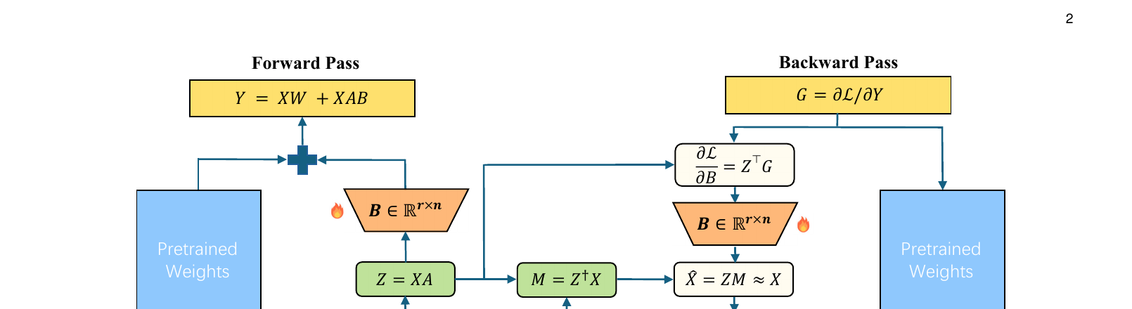
CARE-LoRA does not change LoRA’s forward computation at all — $Y = X(W+AB)$ is computed exactly as before. The only difference is in what gets saved for the backward pass. During the forward pass, while $X$ is still available, CARE-LoRA computes two extra quantities:

$$Z = XA \in \mathbb{R}^{N \times r}, \tag{5}$$ $$M_\lambda^\star = (Z^\top Z + \lambda I_r)^{-1} Z^\top X \in \mathbb{R}^{r \times m}. \tag{6}$$

$Z$ is literally a byproduct of the LoRA forward computation ($X(W+AB) = XW + (XA)B$, so $Z=XA$ is computed regardless). $M$ requires one extra small linear solve — inverting an $r \times r$ matrix, where $r$ is typically 8–64 — which is cheap in both memory and FLOPs relative to anything involving the full $N \times m$ activation. After computing $Z$ and $M$, CARE-LoRA discards $X$ and saves only $Z$ and $M$ for the backward pass. This is the entire memory trick: two small tensors, $N \times r$ and $r \times m$, replace one large tensor, $N \times m$.

3.2 The backward pass: exact gradients for $B$ and $X$, reconstructed gradient for $A$

Given the upstream gradient $G$, the backward pass recomputes an approximate activation

$$\hat{X} = ZM \approx X, \tag{7}$$

and then computes the three gradients as:

$$\nabla_B \mathcal{L} = Z^\top G \quad \text{(exact — identical to Eq. 2)}, \tag{8}$$ $$\widetilde{\nabla}_A \mathcal{L} = \hat{X}^\top G B^\top = M^\top Z^\top (GB^\top) \quad \text{(approximate)}, \tag{9}$$ $$\nabla_X \mathcal{L} = G(W+AB)^\top \quad \text{(exact — identical to Eq. 4, needed to propagate to earlier layers)}. \tag{10}$$

Two points deserve emphasis because they are easy to miss on a first read. First, $\nabla_B \mathcal{L}$ and $\nabla_X \mathcal{L}$ are exactly recovered — CARE-LoRA introduces zero approximation error into the gradient that flows to earlier layers, or into the update for $B$. The only approximated quantity in the entire backward pass is $\nabla_A \mathcal{L}$. This is a much narrower claim than “CARE-LoRA approximates the backward pass,” and it is the reason the method’s accuracy loss (relative to standard LoRA) turns out to be small: only one of the two trainable matrices gets a biased gradient, and even that bias is controlled (Section 3.3). Second, the paper’s implementation never actually materializes the $N \times m$ matrix $\hat{X} = ZM$ — it computes $\widetilde{\nabla}_A \mathcal{L} = M^\top Z^\top (GB^\top)$ directly using the associativity of matrix multiplication, so the largest intermediate tensor touched during the backward pass for $A$‘s gradient is $N \times r$ or $N \times n$, never $N \times m$. This ordering-of-operations detail is what actually delivers the memory saving in practice, not just on paper.

3.3 Algorithm, step by step

Algorithm 1 — CARE-LoRA forward/backward for one adapted linear layer

FORWARD PASS
Input:  activation X ∈ R^(N×m)
State:  frozen weight W ∈ R^(m×n); trainable A ∈ R^(m×r), B ∈ R^(r×n)
Output: Y ∈ R^(N×n); saved tensors Z, M

1:  Z ← X @ A                          # compressed activation (also used by std. LoRA forward)
2:  M ← (Z^T @ Z + λ*I_r)^-1 @ Z^T @ X  # ridge-regularized least-squares reconstruction matrix
3:  ΔY ← Z @ B                          # LoRA branch output
4:  Y ← X @ W + ΔY                      # full layer output
5:  save Z, M ; discard X               # <-- the memory win happens here
6:  continue forward propagation with Y

BACKWARD PASS
Input:  upstream gradient G = ∂L/∂Y ∈ R^(N×n)
State:  saved Z ∈ R^(N×r), M ∈ R^(r×m)
Output: gradients ∇_A~L, ∇_B L, ∇_X L

1:  ∇_X L  ← G @ (W + A@B)^T            # exact — identical to standard LoRA
2:  ∇_B L  ← Z^T @ G                    # exact — identical to standard LoRA
3:  X_hat  ← Z @ M                      # (conceptual only — never materialized in practice)
4:  ∇_A~L  ← M^T @ Z^T @ (G @ B^T)      # reconstructed / approximate gradient for A
5:  update A, B with the optimizer using ∇_A~L, ∇_B L
6:  continue backpropagation with ∇_X L

Walking through why each line matters: line 1 of the forward pass is not new work — it is a value LoRA already computes. Line 2 is the one genuinely new computational step, an $r \times r$ linear solve that costs $O(Nr^2 + mr^2 + r^3)$, negligible next to the $O(Nmr)$ cost of the LoRA matrix multiplications themselves once $r \ll m$. Line 5 (discard $X$) is where the memory accounting changes: the tensor that would have persisted from the forward pass to the backward pass drops from $N \times m$ floats to $(N r + rm)$ floats. In the backward pass, lines 1–2 are unchanged from vanilla LoRA (this is the “no approximation error propagates to earlier layers or to $B$” guarantee), and lines 3–4 are the reconstruction: instead of computing $\nabla_A \mathcal{L} = X^\top G B^\top$ with the (now-discarded) real $X$, it substitutes the reconstructed $\hat{X} = ZM$ into the same formula.

3.4 Why LoRA-FA fails and CARE-LoRA (provably) doesn’t: the subspace-evolution argument

This is the theoretical core of the paper, and it deserves a full derivation because the headline claim — “CARE-LoRA’s projection-down subspace can evolve during fine-tuning” — is not obvious a priori; a naive reader might assume that any reconstruction-based gradient for $A$ is just as constrained as LoRA-FA’s absence of a gradient at all.

Setting up the geometry. Let $S = \mathrm{Col}(A) \subseteq \mathbb{R}^m$ be the current column space of $A$ — an $r$-dimensional subspace of the $m$-dimensional input feature space. Because every column of the LoRA update satisfies $\Delta W_{:,j} = AB_{:,j} \in \mathrm{Col}(A)$, the entire representational capacity of the adapter at a given moment is confined to $S$. LoRA-FA freezes $A$, so $S$ is frozen for the whole training run — whatever directions were captured (or missed) by $A$‘s random initialization is what the adapter is stuck with forever. The natural question for any method that updates $A$ via gradient descent is: does the updated $A^+ = A - \eta \nabla_A \mathcal{L}$ have a column space that is still contained in $S$, or can it escape into new directions?

Deriving the reconstructed gradient in closed form. Starting from Eq. (9) and substituting the closed-form $M$ from Eq. (6):

$$\widetilde{\nabla}_A \mathcal{L} = M^\top Z^\top G B^\top = X^\top Z (Z^\top Z + \lambda I_r)^{-1} Z^\top (GB^\top). \tag{11}$$

Substituting $Z = XA$ throughout:

$$\widetilde{\nabla}_A \mathcal{L} = X^\top X A \left(A^\top X^\top X A + \lambda I_r\right)^{-1} A^\top X^\top (GB^\top) = \Sigma_X A K_\lambda, \tag{12}$$

where $\Sigma_X := X^\top X \in \mathbb{R}^{m \times m}$ is the (unnormalized) second-moment / batch-covariance matrix of the input activations, and

$$K_\lambda := (A^\top \Sigma_X A + \lambda I_r)^{-1} A^\top X^\top U, \qquad U := GB^\top \in \mathbb{R}^{N \times r}. \tag{13}$$

This is the key algebraic fact: the reconstructed gradient factors as $\Sigma_X A$ (a fixed subspace-defining term) times $K_\lambda$ (an $r \times r$ mixing matrix). Everything now hinges on what $\Sigma_X A$ does to the current subspace $S = \mathrm{Col}(A)$.

Why $\Sigma_X A$ can leave the subspace. If $S$ happened to be an invariant subspace of $\Sigma_X$ — meaning $\Sigma_X$ maps every vector in $S$ back into $S$ — then $\Sigma_X A$ would still have all its columns inside $S$, and the gradient step would never escape $\mathrm{Col}(A)$. But $\Sigma_X$ is the covariance structure of the actual training data, and a randomly initialized $r$-dimensional subspace has essentially zero probability of being invariant under an arbitrary $m \times m$ positive semi-definite matrix, except in degenerate cases like $\Sigma_X = cI_m$ (isotropic data — never true in practice for real activations, which have highly structured, anisotropic covariance). Formally, writing $P_S$ and $P_{S^\perp} = I_m - P_S$ for the orthogonal projectors onto $S$ and its complement, the condition for the gradient step to introduce genuinely new directions is

$$D := P_{S^\perp} \Sigma_X A \neq 0. \tag{14}$$

This fails only when $\mathrm{Col}(\Sigma_X A) \subseteq \mathrm{Col}(A)$ — i.e., only in the special invariant-subspace case just ruled out generically.

Why the mixing term $K_\lambda$ doesn’t cancel this. Even with $D \neq 0$, it is conceivable that the right-multiplication by $K_\lambda$ could zero out exactly the off-subspace component. The paper checks this directly: after a gradient step $A^+ = A - \eta \Sigma_X A K_\lambda$, using $P_{S^\perp} A = 0$ (since $A$‘s own columns lie in $S$ by definition),

$$P_{S^\perp} A^+ = -\eta\, P_{S^\perp} \Sigma_X A K_\lambda = -\eta\, D K_\lambda. \tag{15}$$

For this to vanish (i.e., for $A^+$ to stay inside $S$ despite $D \neq 0$), $K_\lambda$ would have to be exactly rank-deficient in a way that cancels $D$‘s row space — a non-generic coincidence. The paper works through the three ways $DK_\lambda$ could vanish (rank-deficient $Z$, rank-deficient $U=GB^\top$, or a non-generic algebraic cancellation between full-rank $Z$ and $U$) and argues each is a measure-zero event for real, non-degenerate training batches. The conclusion: generically, $\mathrm{Col}(A^+) \not\subseteq \mathrm{Col}(A)$ — the subspace moves.

What this buys, and what it doesn’t. This is a genuine structural difference from LoRA-FA (whose subspace literally cannot move, by construction, not just “generically doesn’t”), and it is a nontrivial, non-obvious mathematical fact about the reconstruction scheme — worth taking seriously as a real contribution. But note precisely what is and is not claimed: the argument shows the subspace can move, and generically does move by a nonzero amount, in a data-dependent direction ($\Sigma_X A$). It does not show that the subspace moves toward task-relevant directions, or that it converges to a good subspace, or that it moves fast enough to fully recover standard LoRA’s accuracy. It is a genericity/non-degeneracy argument, not a convergence guarantee — a distinction the empirical section implicitly confirms, since CARE-LoRA at matched rank $r=8$ does not quite match standard LoRA’s accuracy (85.22 vs 85.24 on GLUE, 53.12 vs 53.74 on the Mistral LLM tasks), it only closes most of LoRA-FA’s gap. This is worth holding onto for the critical-analysis section below.

3.5 Design choice discussion: why this particular reconstruction, and not the alternatives?

Why reuse $A$ instead of a separate decomposition (as LoRAct does)? The obvious alternative to CARE-LoRA’s approach is what LoRAct does: run an independent low-rank decomposition of $X$ (its own rank $k$, unrelated to the LoRA rank $r$) purely for activation compression, decoupled from the LoRA computation. This has the advantage of a decomposition rank that can be tuned independently of $r$. But it has two costs CARE-LoRA avoids: (a) it requires an extra decomposition computation (e.g., a randomized SVD or similar) on top of the LoRA forward pass, rather than reusing $Z=XA$, which the LoRA branch computes anyway — this shows up empirically as LoRAct’s 1.38× time overhead versus CARE-LoRA’s 1.02×; (b) more subtly, LoRAct’s decomposition is not tied to the direction $A$ that actually determines the LoRA update, so there is no guarantee that its compressed representation captures the directions that matter for $\nabla_A \mathcal{L}$ specifically — CARE-LoRA’s reconstruction is, by construction, optimized (via the least-squares fit) to best predict $X$ specifically from the LoRA branch’s own $Z$, which is exactly the quantity needed downstream.

Why least-squares (Frobenius) reconstruction rather than a learned reconstruction network? A learned nonlinear decoder (a small MLP mapping $Z \to \hat{X}$) could in principle be more expressive than a linear map $M$. The paper doesn’t take this route, and the reasons are practical: a learned decoder needs its own parameters, its own gradients, and its own optimizer state — reintroducing exactly the kind of overhead CARE-LoRA is trying to eliminate. The closed-form least-squares $M$ requires no additional trainable parameters at all (it’s a deterministic function of $Z$ and $X$, recomputed fresh every forward pass), so it adds zero optimizer-state memory and, being a single matrix solve, minimal compute. The tradeoff is that $M$ is optimal only for the current batch — it is refit every forward pass rather than learned over the whole training trajectory, which is both a strength (no distribution-shift staleness) and a limitation (it cannot amortize information across batches, and must be recomputed at nontrivial — if small — cost every step).

Why does the ridge regularizer matter, and where could it fail? The regularizer $\lambda I_r$ in Eq. (6) prevents the least-squares solve from blowing up when $Z^\top Z$ is ill-conditioned — which happens when the compressed activations across the batch are nearly linearly dependent, e.g., very small batch sizes ($N$ close to or below $r$), or highly repetitive/low-diversity input data within a batch. In those regimes, the reconstruction quality of $\hat{X} \approx X$ degrades, and — following the argument in Section 3.4 — a poorly conditioned $Z$ also risks making $Z^\top U$ closer to the rank-deficient corner case, which is exactly the scenario in which $D K_\lambda$ could vanish and the subspace-evolution guarantee weakens. The paper does not report an ablation over batch size vs. accuracy for this specific interaction, which is a real gap (discussed further below).

Why not simply apply activation quantization (à la HyC-LoRA) to the LoRA branch’s own input? Quantizing $X$ itself (rather than compressing it through $A$) would also save memory, and would apply uniformly regardless of $r$. The reason CARE-LoRA doesn’t do this is architectural fit: LoRA’s $A$ already performs a linear, learned compression of $X$ as a side effect of the forward pass — reusing it costs nothing extra, whereas quantization requires separate calibration/outlier handling machinery (as HyC-LoRA’s design attests) and targets a different axis of redundancy (numerical precision) rather than dimensionality. The two approaches are not mutually exclusive — quantizing $Z$ and $M$ themselves, on top of CARE-LoRA’s dimensionality reduction, is a natural further compression the paper does not explore.

3.6 Where CARE-LoRA sits in the broader PEFT-memory landscape

It is worth stepping back and placing this paper against the wider body of work this blog has already covered on memory-efficient and low-rank training, because CARE-LoRA’s positioning is narrower — and therefore more defensible — than it might first appear. GaLore (reviewed earlier in this series) projects the gradient of a full-parameter fine-tune into a low-rank subspace to save optimizer-state memory, operating on full fine-tuning rather than adapter-based PEFT; it solves a different bucket (bucket 3, optimizer states) for a different training regime (full fine-tuning) via a conceptually similar mechanism (low-rank projection), but the two are not directly substitutable — GaLore doesn’t address LoRA’s activation bottleneck, and CARE-LoRA doesn’t address full-fine-tuning’s optimizer-state bottleneck. AdaLoRA, by contrast, operates squarely within LoRA-style adapters but attacks a different resource: it reallocates the rank budget itself across layers based on an importance score, which is orthogonal to (and in principle combinable with) CARE-LoRA’s activation-memory trick — nothing about CARE-LoRA’s reconstruction mechanism assumes a fixed rank across layers. DoRA and PiSSA, as already discussed, are accuracy-oriented reparameterizations of the LoRA update itself (magnitude/direction decomposition; SVD-based initialization) and share no memory-saving mechanism with CARE-LoRA at all — they are included in the experiments purely as accuracy references. This positions CARE-LoRA as solving a genuinely narrow and previously under-addressed slice of the PEFT memory problem: not parameters, not optimizer states, not rank allocation, but specifically the activation memory retained because both LoRA factors are trainable. That narrowness is a strength, not a weakness — it makes the method easy to reason about, easy to combine with rank-allocation or quantization techniques, and easy to verify the claimed guarantees for, precisely because it changes only one well-defined piece of the training pipeline.

4. Memory and compute cost, derived precisely

4.1 Activation memory

Standard LoRA must retain the entire input activation to compute $\nabla_A \mathcal{L} = X^\top G B^\top$, so the LoRA-branch activation memory is

$$M^{\text{act}}_{\text{LoRA}} = Nm. \tag{16}$$

CARE-LoRA instead saves $Z \in \mathbb{R}^{N\times r}$ and $M \in \mathbb{R}^{r\times m}$:

$$M^{\text{act}}_{\text{CARE}} = Nr + rm = r(N+m). \tag{17}$$

The ratio is

$$\frac{M^{\text{act}}_{\text{CARE}}}{M^{\text{act}}_{\text{LoRA}}} = \frac{r(N+m)}{Nm}. \tag{18}$$

Plugging in the paper’s worked example — T5-Base fine-tuning on MNLI, sequence length 256, batch size 32 so $N = 8192$, hidden size $m = 768$, rank $r=8$:

$$\frac{8 \times (8192 + 768)}{8192 \times 768} = \frac{8 \times 8960}{6{,}291{,}456} \approx 1.14\%. \tag{19}$$

Table 5 in the paper reports the empirically-measured version of this ratio across batch sizes (using $r=16$ against LoRA’s $r=8$, its harder comparison point), and it is instructive because it shows the ratio shrinking as batch size grows: 4.65% at $N$ corresponding to batch size 8, down to 2.46% at batch size 128. This matches Eq. (18) directly: as $N \to \infty$, the ratio $\frac{r(N+m)}{Nm} \to \frac{r}{m}$ (the $rm$ term becomes negligible relative to $rN$, and the ratio approaches a constant depending only on $r/m$), while for small $N$ the fixed $rm$ overhead is proportionally larger. This is a clean, verifiable prediction from the formula, and the empirical numbers confirm it.

4.2 Compute cost

Counting only the LoRA-branch matrix multiplications (both passes), standard LoRA costs

$$T_{\text{LoRA}} = 3Nmr + 3Nrn = 3Nr(m+n). \tag{20}$$

(Three multiplications of cost $Nmr$: the forward $XA$, and two backward terms sharing this shape; three of cost $Nrn$: forward $ZB$ and its two backward counterparts — the paper’s accounting groups them this way without spelling out each term individually, which is a minor expository gap but the total is standard.)

CARE-LoRA’s extra cost comes from solving for $M$ (an $r\times r$ solve applied to $N$- and $m$-sized operands) and using it in the reconstructed $A$-gradient:

$$T_{\text{extra}} = 2Nr^2 + 2mr^2 + r^3, \qquad T_{\text{CARE}} = T_{\text{LoRA}} + T_{\text{extra}}. \tag{21}$$

The relative overhead is

$$\frac{T_{\text{CARE}}}{T_{\text{LoRA}}} = 1 + \frac{r(2N + 2m + r)}{3N(m+n)}. \tag{22}$$

Since $r \ll \min(m,n,N)$ by design, the numerator scales roughly as $r \cdot \max(N,m)$ while the denominator scales as $N \cdot (m+n)$ — as long as $N \gg r$ (always true in practice — batch×sequence tokens vastly outnumber the rank), this ratio stays close to 1. The paper’s worked numeric example (T5-Base, $m=n=768$, $r=8$, $N=8192$) gives

$$\frac{8(2\times 8192 + 2\times 768 + 8)}{3 \times 8192 \times (768+768)} \approx 0.38\%, \tag{23}$$

i.e., a theoretically negligible overhead — consistent with the measured 1.02–1.38× wall-clock ratios reported later (the gap between the ~0.4% theoretical LoRA-branch-only estimate and the measured ~2–38% end-to-end overhead is because the theoretical count only covers LoRA-branch matmuls, not the rest of the transformer block, optimizer step, or memory-allocation/copy overhead — a caveat the paper doesn’t make explicit but that a careful reader should note before treating Eq. (23) as a full training-step estimate).

5. Experiments

The paper evaluates across three genuinely different modalities — NLU (T5-Base), NLG/LLM fine-tuning (Mistral-7B-v0.3), and diffusion personalization (SD3-Medium/DreamBooth) — which is a broader sweep than most PEFT-memory papers attempt, and is one of the paper’s clearer strengths.

5.1 Setup

All methods share backbone, data, target modules, optimizer (AdamW), learning rate, precision, batch size, and training steps within each task, using a common PEFT-based codebase. Results are averaged over three seeds (0, 21, 42) with standard deviations reported. LoRAct’s decomposition rank $k$ is set to 64 (T5-Base) / 128 (Mistral-7B). CARE-LoRA is reported both at matched rank ($r=8$, the fair memory-vs-LoRA-FA comparison) and at a higher rank ($r=16$, the “reinvest the memory savings” comparison against standard LoRA and other accuracy-focused variants).

Figure 1 (paper Fig. 1) below shows the architecture the experiments are built around — the forward pass computing and saving $Z, M$, and the backward pass reconstructing $\hat X$ only for $A$‘s gradient while computing $B$‘s and $X$‘s gradients exactly:

5.2 Natural Language Understanding (GLUE / SuperGLUE, T5-Base, $r=8$)

Figure 2 (paper Tables 1–2) reproduces the head-to-head numbers:

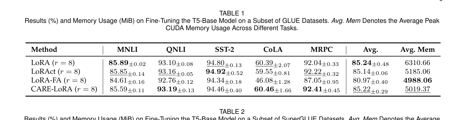
The pattern is consistent across both benchmark suites: CARE-LoRA (85.22 GLUE avg / 78.18 SuperGLUE avg) sits essentially on top of standard LoRA (85.24 / 77.81) — even slightly ahead on SuperGLUE — while LoRA-FA trails badly (80.97 / 70.81). The most dramatic single-task gaps are CoLA (LoRA-FA 46.08 vs. CARE-LoRA 60.46, a 14.4-point swing) and CB (LoRA-FA 76.44 vs. CARE-LoRA 90.03, a 13.6-point swing) — both are small, low-resource tasks where a frozen random subspace is especially likely to miss the directions the task needs, which is exactly the failure mode the subspace-evolution argument in Section 3.4 predicts should be repaired. Memory-wise, CARE-LoRA (5019 MiB GLUE avg) sits within 0.6% of LoRA-FA (4988 MiB) and about 20% below standard LoRA (6311 MiB).

5.3 LLM fine-tuning (Mistral-7B-v0.3: math, code, instruction-following)

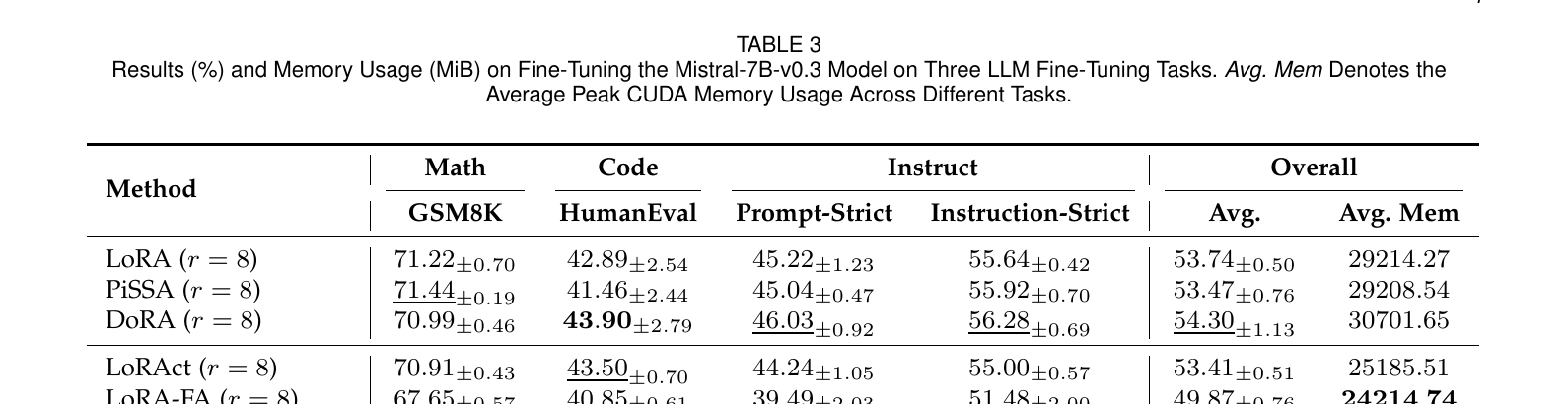
At matched rank ($r=8$), CARE-LoRA (53.12 overall) trails standard LoRA (53.74) by a small margin — this is the residual accuracy gap left by the approximated $\nabla_A\mathcal{L}$ that Section 3.4 flags as a real (if small) cost. But the more interesting comparison is what happens when the saved memory is reinvested into a higher rank: CARE-LoRA at $r=16$ reaches 54.47 overall, the best score among all seven methods compared, including DoRA (54.30, but at 3.39× the per-step time and higher memory) and PiSSA (53.47). This “reinvest memory into rank” framing is one of the paper’s better rhetorical moves — it reframes CARE-LoRA not just as “LoRA-FA but better” but as “a way to afford a higher effective rank than LoRA can afford under the same memory budget,” which is a genuinely different and arguably more useful value proposition.

5.4 Diffusion personalization (SD3-Medium / DreamBooth)

This experiment is the narrowest of the three (only one baseline, standard LoRA, and only two rank settings compared), but it demonstrates the method transfers outside language models to a diffusion-transformer architecture: DINO improves from 43.18 to 43.40, CLIP-I from 69.18 to 69.29, CLIP-T essentially unchanged (28.01 → 28.00), while peak memory drops from 9882 to 8630 MiB (~13%).

5.5 Memory scaling with batch size — the math-visualizing figure

This table is the empirical confirmation of Eq. (18)‘s prediction that the memory ratio should shrink as $N$ grows (because the $rm$ overhead term becomes relatively smaller compared to the $rN$ term as $N$ increases) — the numbers move monotonically from 4.65% down to 2.46% as batch size increases 8→128, which is exactly the qualitative (and roughly quantitative) behavior the formula predicts.

5.6 Time comparison, and the gradient-checkpointing baseline

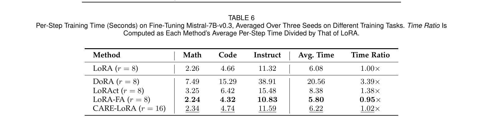
DoRA’s 3.39× overhead comes from combining per-step weight renormalization with backward-pass recomputation in its memory-saving mode — a useful reminder that “memory-efficient” LoRA variants are not automatically fast, and that CARE-LoRA’s near-1.0× time ratio is a genuinely distinguishing property, not a given.

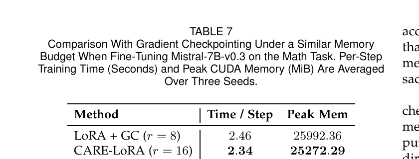
This last comparison is the paper’s argument that CARE-LoRA is structurally better than the generic “recompute activations” fallback: gradient checkpointing recomputes entire transformer blocks (a full extra forward pass through the checkpointed layers) to save memory, whereas CARE-LoRA exploits the LoRA branch’s own low-rank structure to reconstruct only what’s needed — a much cheaper operation per unit of memory saved. The comparison is fair in spirit (matched memory budget) but somewhat narrow in scope: it applies GC to only 8 of 32 decoder blocks (chosen specifically to match CARE-LoRA’s memory footprint), on a single task (Math/GSM8K), so it demonstrates the mechanism is favorable rather than exhaustively characterizing the GC-vs-CARE-LoRA Pareto frontier across checkpointing ratios.

5.7 A closer read of the subspace-evolution claim against the experimental evidence

It is worth explicitly connecting Section 3.4’s theory back to the experimental numbers, since the paper itself does not do this pairing directly. The theory predicts that CARE-LoRA should most clearly outperform LoRA-FA exactly when LoRA-FA’s frozen initial subspace is most likely to be a poor fit for the task — which, all else equal, should be more likely for smaller, more idiosyncratic tasks (where a generic pretrained representation is less likely to already contain task-aligned directions by chance) than for large, generic tasks (where almost any reasonable subspace captures useful signal). This is consistent with the largest CARE-LoRA-vs-LoRA-FA gaps appearing on CoLA (8,551 training examples, a linguistic-acceptability judgment task quite different from the generic language modeling the backbone was pretrained on) and CB (250 examples, extremely low-resource), while the smallest relative gaps appear on the largest, most generic tasks like MNLI (392,702 examples) and QNLI. The theory also predicts, more subtly, that the quality of the reconstructed gradient direction depends on how well $\mathrm{Col}(A)$‘s evolution tracks the directions $\Sigma_X$ actually pushes it toward — which is a property of the data distribution, not of the task label space per se, so this correlation with task size/difficulty is suggestive but not something the paper’s theorem actually proves; it is an empirical pattern consistent with the theory’s spirit, not a validated instance of it. This is exactly the kind of connective analysis a careful reader should perform when a paper presents a theorem and an experiments section somewhat separately, as this one does — and it is also exactly the kind of connective tissue that would strengthen a future revision of the paper if the authors made the link explicitly themselves.

6. Limitations

The paper is reasonably candid about scope but leaves several boundary conditions unexamined:

• Single-layer / single-adapter analysis. All the memory and compute formulas are derived for one adapted linear layer in isolation. The paper doesn’t discuss how the per-layer savings interact with the “shared, fixed-across-methods” costs it excludes from its comparison (model weights, non-LoRA activations, optimizer states) at the level of an entire deep model with dozens of adapted layers — the aggregate effect is presumably close to the per-layer ratio, but this is not shown directly (Table 3’s 18.7% memory savings for the whole Mistral-7B run vs. DoRA is an end-to-end number, but the per-layer accounting in Section 3.4 of the paper is never explicitly reconciled with it).
• Batch-size and conditioning interaction is unexplored empirically. Section 3.4 above already flags that small batch sizes (or low activation diversity) risk ill-conditioned $Z^\top Z$, which both degrades reconstruction quality and — per the subspace argument — could push $DK_\lambda$ closer to the degenerate case where the subspace stops evolving usefully. The paper reports a batch-size sweep for memory (Table 5) but never for accuracy, so we don’t know at what point (if any) small-batch fine-tuning would erode CARE-LoRA’s accuracy advantage over LoRA-FA.
• No interaction with quantized backbones. QLoRA-style 4-bit backbones are mentioned in related work but never combined with CARE-LoRA in experiments — an obvious and practically important combination (quantize $W$, compress activations with CARE-LoRA) is left for future work.
• Rank sensitivity beyond $r \in \{8, 16\}$. All headline numbers use only two rank settings. It’s unclear whether the “reinvest savings into rank” story keeps paying off at $r=32$ or $r=64$, or whether returns diminish (or even reverse, if the least-squares reconstruction quality itself degrades at higher $r$ due to $Z^\top Z$ needing to be inverted in a higher-dimensional space with more potential for ill-conditioning).
• Statistical power on small benchmarks. Several SuperGLUE tasks (CB has 250 dev examples, COPA has 500, WiC and RTE are similarly small) show large standard deviations across seeds (e.g., CB: LoRA-FA $76.44_{\pm 4.92}$, CARE-LoRA $90.03_{\pm 1.40}$) — the paper reports these honestly, but a 13-point average gap on a task with single-run swings of several points, averaged over only 3 seeds, is a noisier signal than the clean headline numbers suggest.

6.1 A deeper look at the reconstruction-error / gradient-bias tradeoff

It is useful to make explicit exactly what kind of error CARE-LoRA introduces, because “approximate gradient” can mean several different things and the paper’s own framing (a single theorem about subspace movement) does not fully characterize the practical error behavior a practitioner should expect. There are two logically distinct sources of imperfection worth separating:

Reconstruction bias. Even with the optimal least-squares $M^\star$, $\hat X = ZM^\star$ is, in general, not equal to $X$ — it is the orthogonal projection of $X$‘s columns onto the column space spanned by $Z$‘s relationship to $X$ within the current batch (more precisely, $ZM^\star$ is the best rank-$r$-consistent linear predictor of $X$ from $Z$ for that batch). Whatever component of $X$ is not linearly predictable from $Z=XA$ is simply lost, and the resulting $\widetilde\nabla_A\mathcal L$ inherits that loss deterministically, batch by batch. This is a bias in the statistical sense: it does not average out over more training steps in the way that gradient noise from mini-batching does, because it is not zero-mean noise — it is a systematic underestimate of the component of the true gradient that depends on the currently-unrepresented part of $X$.

Batch-specific refitting, and its double-edged consequence. Because $M$ is refit fresh every forward pass from the current batch’s $X$ and $Z$, the reconstruction adapts immediately to distribution shift within training (e.g., as fine-tuning data composition changes across an epoch, or across curriculum stages) — there is no staleness of the kind a fixed or slowly-updated decoder would have. But this also means the quality of the reconstruction is only as good as the current batch’s statistics allow, with no memory of how well-conditioned or informative past batches were. A single unusually homogeneous batch (e.g., a batch drawn disproportionately from one sub-task in a multi-task fine-tuning mixture) could transiently produce a low-quality $M$ and a noisier $\widetilde\nabla_A\mathcal L$ for that step, an effect that pure gradient noise from mini-batching would not produce in the same structured way. The paper’s ridge regularization mitigates the worst numerical instability this could cause but does not directly address the representational quality of $M$ in a bad batch — regularization prevents the matrix inversion from blowing up, it does not manufacture information that was not present in a poorly-conditioned batch to begin with.

Practically, this analysis suggests that CARE-LoRA’s accuracy should be somewhat more sensitive than standard LoRA to batch composition and batch size — exactly the empirical gap flagged in Section 5 (Limitations) as unexplored. It also suggests a natural mitigation the paper does not explore: maintaining an exponential moving average of $M$ across recent batches, trading some of the immediate adaptivity to distribution shift for a smoother, lower-variance reconstruction matrix that is less at the mercy of any single batch’s composition — a natural follow-up ablation for future work.

7. Critical analysis

(a) Weaknesses and flaws specific to this paper. The subspace-evolution theorem (Section 3.4) is a genericity argument, not a convergence guarantee, and the paper’s prose occasionally blurs this distinction — phrases like “the projection-down subspace is not frozen” are technically accurate but can be read by a less careful audience as implying the subspace moves in a useful direction, which is never actually shown, only that it moves at all (with probability 1 under non-degenerate data). A theorem proving that $A$‘s subspace is not permanently stuck is a real and useful result, but it is a considerably weaker claim than “CARE-LoRA learns good subspaces,” and the paper’s framing sometimes elides the gap. Separately, the compute-cost analysis in Section 4.2 (Eq. 20–23) is presented only for the LoRA-branch matrix multiplications, but the theoretical ~0.38% overhead estimate is then implicitly compared against measured end-to-end per-step time ratios (1.02–1.38×) without flagging that these numbers are not measuring the same thing — a reader skimming only the equations would come away with an overly optimistic estimate of real-world overhead.

(b) Limitations the authors understate or omit. The paper never discusses what happens under mixed-precision or low-precision training (bf16/fp16), where the ridge regularizer $\lambda$ and the conditioning of $Z^\top Z$ interact with reduced numeric precision — this is exactly the kind of practical detail that determines whether a memory-saving PEFT method is robust in the large-scale training setups where memory savings matter most (very large batch × sequence-length products, often in reduced precision). Likewise, the paper doesn’t discuss how CARE-LoRA composes with other rank-adaptive PEFT techniques like AdaLoRA (which changes $r$ dynamically per layer during training) — since CARE-LoRA’s memory and accuracy properties both depend on $r$, a method that adapts $r$ over time introduces an interaction the paper doesn’t address at all. Finally, the paper reports averages over only three seeds for every experiment; for the smallest SuperGLUE tasks this is a genuinely thin sample for claims of the form “CARE-LoRA achieves the best average score.”

(c) Concrete, specific improvement suggestions. First, the paper would be strengthened by an accuracy-vs-batch-size ablation directly testing the conditioning concern raised in Section 3.5 — e.g., repeating the MNLI experiment at batch sizes 8, 16, 32 and reporting both accuracy and the empirical condition number of $Z^\top Z$, to establish concretely where (if anywhere) the method’s guarantees start to erode. Second, a direct comparison against a learned (rather than per-batch least-squares) reconstruction — even a small ablation with a single trainable linear layer as the decoder instead of the closed-form $M$ — would clarify whether the closed-form solution is leaving meaningful accuracy on the table in exchange for its zero-parameter simplicity, or whether it is already near-optimal for this architecture. Third, given that the paper’s own numbers show a genuinely tighter LLM-scale race (CARE-LoRA at $r=8$ trailing standard LoRA by 0.62 points overall) than the NLU-scale race (CARE-LoRA matching or beating LoRA), an explicit discussion of why the approximation gap seems to widen with backbone/task scale — is it sequence length, task difficulty, or something about Mistral-7B’s activation statistics — would materially improve the paper’s diagnostic value, rather than leaving the reader to notice the pattern independently.

7.1 A note on generality beyond the tested architectures

One question a critical reader should ask of any PEFT-memory paper is: does the mechanism depend on properties specific to the tested architectures, or is it truly architecture-agnostic? CARE-LoRA’s derivation in Section 3 never uses anything about the transformer decoder architecture, the attention mechanism, or the diffusion-transformer structure of SD3 — the entire method is derived for a single generic linear layer $Y = X(W+AB)$ and applies unchanged to any linear layer inside any architecture that uses LoRA-style adapters, including attention projections (Q/K/V/O), MLP up/down projections, and (as the DreamBooth experiment shows) diffusion-transformer blocks. This genuine architecture-agnosticism is a real strength, and it is one of the more convincing pieces of indirect evidence in the paper’s favor — the fact that the same mechanism, with no architecture-specific tuning beyond the rank $r$, produces consistent qualitative behavior (memory reduction with small accuracy cost, closing most of the LoRA-FA gap) across three genuinely different domains (bidirectional encoder-decoder NLU, decoder-only causal LLM fine-tuning, and diffusion-transformer image generation) is a meaningfully stronger generalization signal than a single-architecture ablation would provide, even though each individual domain’s evaluation is comparatively narrow (few tasks, few baselines for the diffusion case in particular).

8. Practical adoption notes

For a practitioner deciding whether to reach for CARE-LoRA, the decision tree implied by the evidence in this paper is fairly clean. If your fine-tuning job is already GPU-memory-bound with standard LoRA — i.e., you are choosing your batch size or sequence length based on activation memory, not compute throughput — CARE-LoRA offers a close-to-free way to either (a) keep the same batch size and rank while cutting memory by roughly 15–20%, freeing headroom for other uses (larger models, more concurrent experiments), or (b) reinvest that headroom into a higher LoRA rank, which the Mistral-7B results suggest is likely to improve accuracy over standard LoRA rather than merely match it. The cases where it is less clearly the right choice: very small batch sizes (where the least-squares reconstruction matrix $M$ is fit from few samples and risks the ill-conditioning discussed in Section 3.5), extremely short sequences where activation memory was never the bottleneck to begin with (in which case the parameter/gradient/optimizer-state buckets already dominate and none of the activation-memory tricks discussed here matter much), or settings where you already use aggressive gradient checkpointing for other reasons (in which case CARE-LoRA’s marginal benefit narrows, per the Table 7 comparison, though it still wins on both memory and speed in the one setting tested).

One practical detail worth flagging for implementers: because $M$ is refit from scratch every forward pass via a small matrix inversion, CARE-LoRA introduces a data-dependent numerical operation into every training step that standard LoRA does not have. This means that unlike LoRA’s forward pass (which is purely deterministic matrix multiplication, easily fused and highly amenable to standard kernel-level optimization), CARE-LoRA’s forward pass has a small control-flow-adjacent cost (solving a linear system, even a tiny $r\times r$ one) that may interact less favorably with some compilation/fusion pipelines (e.g., torch.compile, custom CUDA graphs) than a pure matmul-only forward pass would. The paper’s measured 1.02× overhead suggests this is a non-issue in the tested setups, but it is a detail worth benchmarking specifically if adopting CARE-LoRA inside a heavily kernel-fused training stack rather than a standard eager-mode PyTorch loop.

8.1 A minimal implementation sketch

For readers who want to prototype the idea rather than use the authors’ released code directly, it is worth noting how little needs to change relative to a standard LoRA layer implementation. A standard LoRA linear layer’s forward method computes y = x @ w + (x @ A) @ B and relies on autograd to handle the backward pass by keeping x alive. To convert this into a CARE-LoRA layer, the forward method instead needs to: (1) compute z = x @ A as before; (2) solve the small ridge regression M = torch.linalg.solve(z.T @ z + lam * I, z.T @ x), an $r \times r$ system regardless of how large $m$ is; (3) register z and M (not x) as the tensors saved for backward, typically via a custom torch.autograd.Function with an explicit backward method rather than relying on vanilla autograd (since the whole point is to avoid the default behavior of keeping x alive); and (4) in the custom backward, compute grad_B = z.T @ grad_output, grad_x = grad_output @ (w + A @ B).T exactly as standard LoRA would, and grad_A = M.T @ z.T @ (grad_output @ B.T) in place of the standard x.T @ grad_output @ B.T. The engineering delta is genuinely small — one linear solve and a custom autograd function — which is consistent with the paper’s reported near-1.0× time overhead and suggests the method should be straightforward to retrofit into existing LoRA implementations (e.g., Hugging Face peft) without a large engineering investment, an underappreciated practical virtue relative to methods that require deeper changes to the training loop (like gradient checkpointing’s need to control which blocks are recomputed, or quantization-based approaches’ need for calibration passes).

9. Conclusion

CARE-LoRA makes a narrow, well-targeted observation — once you fix everything else that LoRA already fixes, the last activation-memory tax is the full input $X$ needed only for $\nabla_A \mathcal{L}$ — and answers it with a genuinely elegant mechanism: reuse the LoRA branch’s own compressed activation $Z=XA$, fit the cheapest possible linear decoder $M$ back to $X$ via ordinary least squares, and accept the resulting gradient approximation only where it’s unavoidable (the gradient of $A$), while keeping every other gradient exact. The subspace-evolution derivation is the paper’s most substantive theoretical contribution and correctly identifies why LoRA-FA’s frozen-subspace failure mode is avoidable in principle, even though the result is a genericity argument rather than a convergence guarantee. Empirically, the method delivers on its promise across three different modalities (NLU, LLM fine-tuning, diffusion personalization) with close-to-LoRA-FA memory and close-to-LoRA accuracy, and its “reinvest the savings into a higher rank” framing turns an activation-memory trick into a genuine method for buying more expressive adapters under a fixed hardware budget — arguably the more practically important framing of the two results the paper reports.

Appendix: Reading the memory ratio formula as a design knob

One last piece of intuition worth spelling out, because it clarifies exactly what a practitioner controls when adopting CARE-LoRA: rewrite Eq. (18) as

$$\frac{M^{\text{act}}_{\text{CARE}}}{M^{\text{act}}_{\text{LoRA}}} = \frac{r}{m} + \frac{r}{N}. \tag{24}$$

This decomposition (obtained by splitting $\frac{r(N+m)}{Nm}$ into $\frac{rN}{Nm} + \frac{rm}{Nm}$) makes the two knobs a practitioner actually controls explicit. The first term, $r/m$, is fixed once the rank and hidden width are chosen — it is the asymptotic floor the ratio approaches as batch size grows without bound, and it is entirely a property of the adapter configuration, not of the data or batch. The second term, $r/N$, is the part that shrinks as batch size (or sequence length, since $N$ is their product) increases — this is exactly why Table 5’s empirical ratios keep falling as batch size grows, and it tells a practitioner precisely when CARE-LoRA’s relative memory advantage is largest: short-sequence, small-batch fine-tuning runs (where $r/N$ dominates and is itself still small relative to $r/m$ only if $N$ is not too small) benefit less in relative terms than long-sequence, large-batch runs, but since $r/m$ is already the dominant term for realistic ranks (e.g., $r=16$, $m=4096$ gives $r/m \approx 0.4\%$), the practical takeaway is that CARE-LoRA’s memory benefit is fairly stable across the batch-size/sequence-length regimes practitioners are likely to encounter, with the batch-size dependence mattering most only at unusually small $N$ — precisely the regime flagged in Sections 3.5 and 6 as also being where the least-squares reconstruction is least numerically reliable. These two independent lines of reasoning (the memory-ratio formula and the conditioning analysis) point at the same operating boundary from different directions, which is a reassuring internal consistency check on the overall design, even though the paper itself never states Eq. (24) in this decomposed form or draws this connection explicitly.

Reproducibility notes

• Code is publicly available at https://github.com/fishandyu/CARE-LoRA.
• All experiments use a unified PEFT-based codebase (Hugging Face peft), AdamW optimizer, and three fixed seeds (0, 21, 42), with the same backbone/data/target-modules/precision/batch-size/steps held constant across methods within each task — a reasonably controlled setup for reproduction.
• The only method-specific hyperparameters to reproduce are: CARE-LoRA’s ridge regularizer $\lambda$ (reported as “a very small value,” not stated numerically in the main text — a gap for exact reproduction) and LoRAct’s decomposition rank $k$ (64 for T5-Base, 128 for Mistral-7B-v0.3).
• Benchmarks used: GLUE (MNLI, QNLI, SST-2, CoLA, MRPC), SuperGLUE (BoolQ, CB, COPA, RTE, WiC), MetaMathQA→GSM8K, OpenCodeInstruct→HumanEval, SmolTalk→IFEval, and DreamBooth (10 fixed subjects, DINO/CLIP-I/CLIP-T metrics) — all are standard, publicly available benchmarks, which supports reproducibility.