KV Cache Compression Through the Lens of Transform Coding: What AATC Gets Right About Attention-Aware Quantization

Review date: 2026-08-19 Author: Zhongzhu Zhou Paper reviewed: KV Cache Compression Through the Lens of Transform Coding Paper authors: Hannah Laus, Claudio Mayrink Verdun, Hao Wang, Flavio du Pin Calmon, Felix Krahmer (TU Darmstadt / TU Munich / MCML; MIT; Red Hat AI Innovation Team & MIT-IBM Watson AI Lab; Harvard University) arXiv: 2608.14191 Venue/Status: Preprint (cs.LG), August 2026

1. The question this paper actually asks

Most KV cache quantization papers implicitly answer a question that sounds right but is subtly wrong: “how do I represent the cached keys and values with as few bits as possible while keeping them close to their original values?” That is the reconstruction-error question. AATC (Attention-Aware Transform Coding) starts from a different, more precise question: “how do I represent the cached keys and values with as few bits as possible while keeping the attention output close to what it would have been with full-precision keys and values?” These two questions have different answers, and the gap between them is exactly where AATC finds its improvement.

Why does the distinction matter in practice? Because attention does not treat every key-value pair, and every channel of every key-value pair, symmetrically. A key channel that the current query almost never reads from can be quantized to garbage without moving the attention output at all; a token that receives near-zero attention weight can have its value quantized coarsely for free. Reconstruction-error-minimizing quantizers cannot see this — they treat every coordinate as equally important because their objective function has no term that references the query, the output projection, or the attention weights. AATC’s central contribution is a theorem that makes this asymmetry explicit and differentiable enough to optimize against: a closed-form decomposition of the attention output distortion into additive key and value contributions, each of which further factors into a token-dependent part and a channel-dependent part. Once you have that decomposition, the bit-allocation problem becomes a textbook rate-distortion problem, and the paper solves it with 1950s-vintage tools — transform coding and reverse waterfilling — updated with a 2020s-vintage twist: the “signal” is not raw KV data, it is KV data as perceived through the query and the output projection.

This review works through the paper in three passes. First, we build up the prerequisite background: what the KV cache actually stores, what quantization does to it, and what transform coding and reverse waterfilling are (if you have read a classical information theory textbook you can skim this, but it is worth being precise since AATC borrows the machinery verbatim). Second, we derive the paper’s main theorem in detail, because the theorem is the paper’s real contribution and the algorithm itself is a fairly mechanical consequence of it. Third, we walk through the algorithm, the experimental results, and the design choices the authors made (and the ones they didn’t), before giving an independent critical assessment.

2. Prerequisites

2.1 Why the KV cache exists and why it grows

A decoder-only transformer generates text one token at a time. At layer $\ell$, each token’s hidden vector is linearly projected into a query $q_t$, a key $k_t$, and a value $v_t$. Self-attention computes, for the current query, a similarity score against every key seen so far, turns those scores into a probability distribution via softmax, and returns the corresponding weighted average of the values:

$$\mathrm{Attention}(q_t, K_{\le t}, V_{\le t}) = \Big(\sum_{i \le t} a_{ti} v_i\Big) W_O, \qquad a_{ti} = \frac{\exp(q_t^\top k_i / \sqrt{d_k})}{\sum_{j \le t} \exp(q_t^\top k_j / \sqrt{d_k})}. \tag{1}$$

During autoregressive decoding, token $t+1$‘s query needs to attend to all keys and values from tokens $1, \dots, t$, not just the newest one. Recomputing $k_i, v_i$ for every past token at every decoding step would mean $O(t)$ redundant work per step, so instead every key and value ever computed is cached: the KV cache at decoding step $t$ is $\{(K_{\le t}^{(\ell)}, V_{\le t}^{(\ell)}) \mid \ell \in [L]\}$, one pair of growing matrices per layer. This cache’s memory footprint grows linearly with the number of tokens processed so far, and at long context lengths (the paper cites contexts exceeding a million tokens for modern deployments) it dwarfs the memory used by the model’s own weights. Compressing this cache without hurting generation quality is therefore one of the highest-leverage engineering problems in LLM serving, and it is why every major inference stack (vLLM, SGLang, TensorRT-LLM) ships some form of KV cache quantization or eviction.

To put concrete numbers on this: Llama-3.1-8B-Instruct has 32 layers, 8 KV heads, and a per-head dimension of 128, so each token contributes $32 \times 8 \times 128 \times 2\,(\text{K and V}) = 65{,}536$ FP16 values, i.e., 128 KB per token. A single 32k-token context therefore needs roughly 4 GB of cache per concurrent request — more than a fully quantized 7B model’s own weights — and this scales linearly with however many requests a server is batching concurrently. This is exactly the number the paper reports shrinking from 1.07 GB (FP16, for a shorter representative sequence) down to 184 MB at its 5.82x operating point in Section 6.2 below, and it is why a serving-side memory budget, not accuracy alone, is often the binding constraint that determines how many concurrent long-context requests a GPU can actually hold in memory at once.

2.2 Scalar quantization, precisely

The paper uses the standard uniform scalar quantizer. Given a scale $\Delta > 0$ and a zero-point $z$, a $b$-bit quantizer maps a real number $x$ to an integer code and back:

$$\mathrm{qtz}(x) = \mathrm{clamp}\left(\left\lfloor \frac{x - z}{\Delta} + \frac{1}{2} \right\rfloor,\ 0,\ 2^b - 1\right), \qquad \mathrm{dqtz}(c) = \Delta \cdot c + z. \tag{2}$$

The reconstruction $\hat{x} = \mathrm{dqtz}(\mathrm{qtz}(x))$ satisfies $|x - \hat{x}| \le \Delta/2$ as long as $x$ falls within the clipping range — this is the basic guarantee that lets you reason about quantization error as a bounded, roughly uniform random variable. Applying this per-element to keys and values gives quantized caches $\hat{k}_i = \mathrm{dqtz}(\mathrm{qtz}(k_i))$, $\hat{v}_i = \mathrm{dqtz}(\mathrm{qtz}(v_i))$, with error vectors $\delta k_i = \hat{k}_i - k_i$, $\delta v_i = \hat{v}_i - v_i$. The scale $(\Delta, z)$ can be shared per-tensor, per-token, or per-channel; existing methods like KIVI mix these granularities (per-channel for keys, per-token for values) because keys and values have empirically different outlier structures.

2.3 Transform coding and reverse waterfilling, from first principles

This is the part of the paper’s toolkit that is genuinely 70 years old, and it is worth deriving because AATC’s “innovation” is largely about what quantity you plug into this machine, not the machine itself.

Suppose you have a zero-mean random vector $x \in \mathbb{R}^d$ with covariance $\Sigma$, and you want to represent it with an average of $\bar{b}$ bits per dimension so as to minimize the mean squared error $D = \frac{1}{d}\mathbb{E}\|x - \hat{x}\|_2^2$. If you quantize each coordinate of $x$ independently in the original basis, you waste bits: highly correlated coordinates carry redundant information, so you are effectively paying twice for the same bit of information. Transform coding fixes this in two steps.

flowchart LR
    subgraph Step1["Step 1: Decorrelate"]
        X["Correlated source x\ncovariance Sigma"] --> U["Orthonormal transform\ny = U^T x"]
        U --> Y["Decorrelated coefficients\nvariances sigma_1^2 >= ... >= sigma_d^2"]
    end
    subgraph Step2["Step 2: Allocate"]
        Y --> W["Reverse waterfilling against\ninverted energy landscape\nlog2(1/sigma_i^2)"]
        W --> B["Per-coefficient bits b_i*\nzero bits below water level"]
    end
    B --> Q["Quantize each y_i\nindependently at b_i* bits"]
    Q --> R["Reconstruct: x_hat = U y_hat"]

Figure 1 sketches this classical two-step pipeline, which AATC reuses verbatim; the only thing that changes downstream is which quantity plays the role of the coordinate variance in the waterfilling step.

Step 1 — decorrelate. Apply an orthonormal transform $y = U^\top x$ that diagonalizes the covariance, i.e., $U^\top \Sigma U = \mathrm{diag}(\sigma_1^2, \dots, \sigma_d^2)$. Because $U$ is orthonormal, it preserves squared-error distortion exactly: quantizing $y$ and inverse-transforming back to $\hat{x} = U\hat{y}$ gives the same distortion as if you had quantized $y$ directly. The optimal choice of $U$ for a Gaussian source is the Karhunen–Loève transform — the eigenbasis of $\Sigma$ — which is exactly the PCA basis. In practice $\Sigma$ is estimated from a calibration sample.

Step 2 — allocate. Now that the coordinates $y_1, \dots, y_d$ are decorrelated with variances $\sigma_1^2 \ge \dots \ge \sigma_d^2$, distribute the $\bar b \cdot d$ total bits across them. Under the standard high-rate approximation, a scalar quantizer using $b_i$ bits on a coordinate with variance $\sigma_i^2$ achieves distortion $D_i \approx c\,\sigma_i^2 2^{-2b_i}$ for a quantizer-dependent constant $c$. Minimizing $\frac{1}{d}\sum_i D_i$ subject to $\frac{1}{d}\sum_i b_i = \bar b$ and $b_i \ge 0$ is a constrained convex optimization problem, and its solution is the classical reverse waterfilling allocation:

$$b_i^\star = \begin{cases} \frac{1}{2}\log_2(\sigma_i^2 / \lambda), & \sigma_i^2 > \lambda \\ 0, & \text{otherwise}, \end{cases} \tag{3}$$

where the water level $\lambda > 0$ is chosen so that $\frac{1}{d}\sum_i b_i^\star = \bar b$. Intuitively: imagine pouring a fixed volume of “bit budget” into a container whose base height at position $i$ is $\log_2(1/\sigma_i^2)$ (an inverted energy landscape) — the water settles at a common level $\lambda$, and the depth of water above the base at position $i$ is proportional to the bits allocated there. Coordinates whose variance is below the water level get zero bits — they are reconstructed as zero, i.e., dropped entirely. This is the origin of the “rank reduction as a side effect of bit allocation” phenomenon that shows up later in the paper (Remark 5 in the original text): once the allocation is solved, some transformed dimensions simply receive no bits, which is mathematically equivalent to a data-dependent, adaptively-sized low-rank truncation, without ever explicitly deciding on a rank ahead of time.

Two things to notice about this classical solution, because both get modified by AATC. First, every retained coefficient is quantized to the same distortion $c\lambda$ — this is the “water level” intuition made precise: bits go where they reduce distortion the most, until the marginal benefit equalizes everywhere. Second, the whole derivation assumed you were minimizing reconstruction distortion on $x$ itself. If what you actually care about is some downstream function of $x$ — here, the attention output computed from $x$ — then the "$\sigma_i^2$" that should go into equation (3) is not the raw coordinate variance but a weighted variance that reflects how much that coordinate matters to the downstream function. This is precisely the gap AATC closes.

2.4 What existing KV cache quantization methods optimize instead

Before AATC, KV cache compression methods clustered into a few families that the paper is careful to place on a common footing (Table I in the original, reproduced below in Section 5):

• Scalar quantization (KIVI, KVQuant): quantize every key/value coordinate independently, with per-channel or per-token scales, sometimes with non-uniform codebooks and outlier handling — but the bits assigned to each channel are uniform or heuristically tuned, not derived from an explicit distortion objective on the output.
• Vector quantization (A2ATS, CommVQ, TurboQuant): jointly quantize groups of coordinates via learned codebooks.
• Low-rank / transform-based methods (PALU, Eigen Attention, xKV): decorrelate along the feature dimension and delete low-energy subspaces outright — a hard, fixed-rank truncation decided in advance, not adapted to the available bit budget.
• Transform-coding methods (KVTC, the closest prior work to AATC): decorrelate the cache and allocate bits by reverse waterfilling, exactly like AATC — but the distortion objective they minimize is the raw reconstruction error $\mathbb{E}\|k_i - \hat k_i\|^2$, $\mathbb{E}\|v_i - \hat v_i\|^2$, which the KVTC authors themselves acknowledge is only a proxy for the quantity that actually matters.
• Eviction methods (H2O, SnapKV, StreamingLLM): drop entire tokens based on attention-score-derived importance criteria.
• Rotation-based methods (OSCAR, and the query-aware rotation line of work): apply an orthogonal transform before quantization specifically chosen to make the query-facing geometry more quantization-friendly.

AATC’s positioning claim is that all of these are optimizing projections of a single underlying distortion quantity, just from different angles, and that once you write down that quantity in closed form, you can allocate bits against all of its structure at once rather than picking one axis and optimizing it in isolation.

3. Theorem 1: deriving the attention-aware distortion

This is the mathematical heart of the paper, so it is worth walking through the full derivation rather than just quoting the result — understanding why the decomposition is additive (no cross-terms between key and value errors) is what lets you trust the resulting bit-allocation formula.

3.1 Setup and assumptions

Fix a single decode step and drop the layer index for readability. The unperturbed attention output for the current token is $o = \sum_{i=1}^{T} a_i v_i W_O$ where $a_i$ are the (unperturbed) attention weights from equation (1). Quantization replaces $k_i \to \hat k_i = k_i + \delta k_i$ and $v_i \to \hat v_i = v_i + \delta v_i$, producing a perturbed output $\hat o = \sum_i \hat a_i \hat v_i W_O$ where $\hat a_i$ are the attention weights recomputed from the perturbed keys.

The analysis rests on two assumptions:

• Assumption 1 (white-noise quantization model). The quantization errors $\delta k_{ic}, \delta v_{ic}$ (subscript $c$ for channel) are zero-mean, mutually independent across tokens and channels, independent between keys and values, and symmetrically distributed (so all odd moments vanish). This is the standard idealization behind rate-distortion analyses of quantization; it is known to be exact only in the high-rate limit, but the paper’s own experiments show the resulting distortion metric remains predictive down to 2–4 bits.
• Assumption 2 (bounded key error). There is a constant $\kappa \ge 1$ such that $|\delta k_{ic}| \le \kappa \sigma_K$ almost surely for every token $i$ and channel $c$, where $\sigma_K^2 := \max_{i,c}\mathbb{E}[(\delta k_{ic})^2]$. This holds automatically for the uniform scalar quantizer of equation (2) because the quantization step scales with the maximum entry per token (via the “right scaling” procedure described in Section 4).

3.2 Step 1 — decompose the output error into three pieces

Write $\delta a_i := \hat a_i - a_i$ for the attention-weight perturbation induced by the key error. Expanding the product $(a_i + \delta a_i)(v_i + \delta v_i)$ and subtracting the unperturbed term, the output error splits into three additive pieces:

$$o - \hat o = -\underbrace{\sum_{i=1}^{T} \delta a_i\, v_i W_O}_{=: E_K} + \underbrace{\sum_{i=1}^{T} a_i\, \delta v_i W_O}_{=: E_V} + \underbrace{\sum_{i=1}^{T} \delta a_i\, \delta v_i W_O}_{=: E_\times}. \tag{4}$$

$E_K$ captures the effect of key quantization through the perturbed attention weights — it is where the softmax nonlinearity enters. $E_V$ captures the effect of value quantization directly (values enter the output linearly, so no nonlinearity intervenes here). $E_\times$ is a second-order cross-term. Since $\mathbb{E}\|o-\hat o\|^2 = \mathbb{E}\|E_K + E_V + E_\times\|^2$, expanding this square produces the two “pure” terms $\mathbb{E}\|E_K\|^2$, $\mathbb{E}\|E_V\|^2$ plus three cross terms $2\mathbb{E}[E_K E_V^\top]$, $2\mathbb{E}[E_K E_\times^\top]$, $2\mathbb{E}[E_V E_\times^\top]$.

3.3 Step 2 — the cross-terms between key and value error vanish

This is the step that makes the “additive key + value” claim of the theorem true, and it is worth seeing why it is not an approximation but an exact algebraic fact for two of the three cross-terms. Because $\delta a_i$ depends only on the key perturbations $\{\delta k_m\}$, and Assumption 1 makes key and value errors independent, $\mathbb{E}[\delta a_i \, \delta v_\ell] = \mathbb{E}[\delta a_i]\,\mathbb{E}[\delta v_\ell] = 0$ for every $i, \ell$ (using $\mathbb{E}[\delta v_\ell] = 0$). Plugging this into the two cross-terms $\mathbb{E}[E_K E_V^\top]$ and $\mathbb{E}[E_K E_\times^\top]$ — both of which are sums of terms containing a factor $\mathbb{E}_{\delta v}[\delta v_\ell]$ — makes them vanish exactly, at every order, not just to leading order. The remaining cross-term $\mathbb{E}[E_V E_\times^\top]$ and the “pure” cross-term $\mathbb{E}\|E_\times\|^2$ do not vanish exactly, but the paper bounds both as $O\big((\|q\|^2\sigma_K^2 + A_0^3)\|W_O\|_F^2\sigma_V^2\big)$ where $A_0 := \kappa\|q\|_1\sigma_K$ is a pathwise bound on the key-induced logit perturbation — this bound is quartic-or-higher in the noise scales $\sigma_K, \sigma_V$, so it is genuinely a higher-order remainder relative to the leading $\mathbb{E}\|E_K\|^2$ and $\mathbb{E}\|E_V\|^2$ terms, which are only quadratic.

3.4 Step 3 — the value distortion term (exact, no expansion needed)

Because values enter linearly (no softmax in the way), this term requires no approximation at all. Expanding $\mathbb{E}\|E_V\|^2 = \sum_{i,\ell} a_i a_\ell\, \mathbb{E}[(\delta v_i W_O)(\delta v_\ell W_O)^\top]$ and using token independence and zero mean, all off-diagonal ($i \ne \ell$) terms vanish, leaving

$$D_V := \mathbb{E}\|E_V\|^2 = \sum_{i,c} a_i^2\, \mathbb{E}[(\delta v_{ic})^2]\, \|W_{O_c}\|_F^2, \tag{5}$$

where $W_{O_c}$ is the $c$-th row of the output projection matrix. Read this formula left to right: the distortion contributed by value channel $c$ of token $i$ is the squared attention weight $a_i^2$ (how much the token matters), times the quantization noise variance in that channel $\mathbb{E}[(\delta v_{ic})^2]$ (how coarsely you quantized it), times the squared norm of the output projection’s row for that channel $\|W_{O_c}\|^2$ (how much that channel’s error gets amplified on its way to the output). All three factors are independently meaningful and none of the pre-AATC scalar quantizers use the third one.

3.5 Step 4 — the key distortion term (needs a softmax Taylor expansion)

Because key errors act through the softmax, this term requires more care. First, recenter each value by the (constant) output $o$: define $u_i := v_i W_O - o$. Because $\sum_i \delta a_i = 0$ exactly (both $\hat a$ and $a$ are probability distributions summing to one), you can substitute $v_i W_O \to u_i$ inside $E_K$ without changing anything. Then Taylor-expand the softmax response along the ray from the unperturbed logits $s$ to the perturbed logits $s + \alpha$ (where $\alpha_i := q^\top \delta k_i = \sum_c q_c \delta k_{ic}$ is the scalar logit perturbation caused by the key error at token $i$):

$$\delta a_i = \underbrace{a_i(\alpha_i - \bar\alpha)}_{\delta a_i^{(1)},\ \text{linear in } \alpha} + \underbrace{\tfrac{1}{2}a_i\big[(\alpha_i - \bar\alpha)^2 - \textstyle\sum_\ell a_\ell(\alpha_\ell - \bar\alpha)^2\big]}_{\delta a_i^{(2)},\ \text{quadratic in } \alpha} + r_i, \tag{6}$$

where $\bar\alpha := \sum_\ell a_\ell \alpha_\ell$ is the attention-weighted mean perturbation and $r_i$ is the exact Taylor remainder past second order. The linear term $\delta a_i^{(1)}$ contributes the leading-order distortion; the quadratic term $\delta a_i^{(2)}$ turns out to contribute zero to the expectation of the key-distortion cross-term (Step 2’s Equation (23) in the original text: the cross term $\mathbb{E}[E_K^{(1)} (E_K^{(2)})^\top]$ reduces to a sum of third-order moments of $\alpha$, each of which is either a product of independent zero-mean factors, or $\mathbb{E}[\alpha_p^3] = 0$ by the symmetry assumed in Assumption 1 — so it vanishes exactly, not just approximately). The Taylor remainder $r_i$ is bounded pathwise by a softmax tail bound (the paper’s Lemma 1): $|r_i| \le 7 A_0^3$ for every token, derived by bounding the third derivative of the softmax response along the ray uniformly and integrating the Taylor remainder formula.

Substituting the leading linear term $\delta a_i^{(1)} = a_i(\alpha_i - \bar\alpha)$ into $E_K = \sum_i \delta a_i u_i$, using $\sum_i a_i u_i = 0$ (again because $u_i$ is centered by construction) to kill the $\bar\alpha$ term, and using $\mathbb{E}[\alpha_i\alpha_\ell] = \delta_{i\ell}\mathbb{E}[\alpha_i^2]$ (independence across tokens) plus $\mathbb{E}[\alpha_i^2] = \sum_c q_c^2 \mathbb{E}[(\delta k_{ic})^2]$ (from equation 10 in the derivation, itself following from channel independence), you get

$$D_K := \mathbb{E}\|E_K\|^2 = \sum_{i,c} a_i^2\, \|v_i W_O - o\|^2\, q_c^2\, \mathbb{E}[(\delta k_{ic})^2]. \tag{7}$$

Again read this left to right: the distortion contributed by key channel $c$ of token $i$ is the squared attention weight $a_i^2$, times how much the output would change if attention mass moved onto or off token $i$ — the residual $\|v_i W_O - o\|^2$ — times the quantization noise in that key channel, times the squared query component in that channel $q_c^2$ (how strongly the current query actually reads that direction). This residual term $\|v_iW_O - o\|^2$ is subtle and easy to miss: it is not “how large is token $i$‘s contribution” (that is $a_i$‘s job), it is “how different is token $i$‘s value from the current output” — a token whose value happens to closely match the attention output anyway is forgiving of key errors, because misallocating attention onto or away from it barely moves the average.

3.6 Putting it together

$$D = \mathbb{E}\|o - \hat o\|^2 = D_K + D_V + R, \qquad |R| \le C\|q\|^2\|W_O\|_F^2\sigma_K^2\sigma_V^2 + C A_0^3\|W_O\|_F^2\sigma_V^2 + D_o A_0^4, \tag{8}$$

with $D_o := \max_i \|v_i W_O - o\|^2$ and $C$ an absolute constant. The remainder $R$ vanishes asymptotically as the quantization noise shrinks and is empirically negligible at the operating bit-widths the paper tests (2–5 bits). The crucial structural fact, visible directly in equations (5) and (7), is that the distortion factorizes into a token-dependent part and a channel-dependent part:

$$D_K = \sum_i \underbrace{a_i^2 \|v_iW_O - o\|^2}_{\text{token factor}} \cdot \sum_c \underbrace{q_c^2\, \mathbb{E}[(\delta k_{ic})^2]}_{\text{channel factor}}, \qquad \text{(analogously for } D_V\text{)}. \tag{9}$$

This factorization is the theorem’s real payoff: it means channel-wise bit allocation (which channels get how many bits) and token-wise operations (eviction, windowing) can be designed independently, because neither factor’s optimum depends on the other. AATC exploits exactly the channel-wise half of this factorization; it leaves the token-wise half (eviction) out of scope, explicitly noting this as future work to combine with the channel allocation.

4. Where this fits relative to prior work: the distortion-factor map

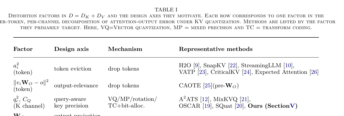
Table I (Figure 2 above) is the paper’s map of the whole KV-compression literature onto the five factors that appear in equations (5) and (7): the token-level attention weight $a_i^2$ (targeted by eviction methods like H2O, SnapKV, StreamingLLM), the token-level output-relevance residual $\|v_iW_O - o\|^2$ (targeted almost uniquely by CAOTE, which works in pre-$W_O$ value space rather than the paper’s residual-stream space), the channel-level query-alignment $q_c^2$ (targeted by A2ATS, MixKVQ, OSCAR, SQuat through various rotation/mixed-precision mechanisms), the channel-level output-projection sensitivity $W_{O_c}$ (which the paper claims no prior method exposes as an explicit allocation factor — it appears only implicitly, entangled with other gradients, in KVQuant’s Fisher-sensitivity weighting), and the classical per-channel quantization sensitivity $\mathbb{E}[(\delta k_{ic})^2], \mathbb{E}[(\delta v_{ic})^2]$ (targeted by essentially every scalar/vector quantization method, including KIVI, KVQuant, and KVTC).

The synthesis claim is specific and falsifiable: AATC is the first method to combine all four channel-level factors ($q_c^2$, $W_{O_c}$, and the two per-channel sensitivities) into a single allocation criterion derived from a closed-form decomposition, rather than picking one factor and addressing it through a bespoke mechanism. Whether this actually buys you something empirically (as opposed to being a nice unification with no practical bite) is exactly what Section 6’s “AATC var-only” ablation is designed to test — spoiler: it buys you something specifically at aggressive compression ratios and specifically on the harder-to-compress model.

A compact way to summarize the field’s coverage of Table I’s five factors, with each representative method’s core mechanism:

Method	Token axis ($a_i^2$ / relevance)	Channel axis (query / output)	Per-channel sensitivity	Allocation basis
StreamingLLM / H2O / SnapKV	Hard eviction by attention magnitude	—	—	Heuristic threshold
CAOTE	Output-relevance residual (pre-$W_O$)	—	—	Closed-form eviction score
A2ATS / MixKVQ / SQuat	—	Query-aware rotation or projection	Implicit via rotation	Fixed precision post-rotation
OSCAR	—	Query-covariance eigenrotation	Implicit via rotation	Uniform INT2 post-rotation
KIVI	—	—	Per-channel (K) / per-token (V) scale	Fixed uniform bits
KVQuant	—	Implicit (entangled in Fisher gradient)	Non-uniform codebook, outlier handling	Sensitivity-weighted codebook
PALU	—	—	SVD truncation (fixed rank)	Fixed-rank cutoff, no allocation
KVTC	—	—	Global cross-layer PCA + allocation	Reverse waterfilling on reconstruction error
AATC (ours)	Out of scope (future work)	Explicit $q_c^2$ and $W_{O_c}$	Per-layer whitening + weighted variance	Reverse waterfilling on output-aware distortion

Reading down the last column is the clearest way to see AATC’s actual claim: it is not the first to use reverse waterfilling (KVTC already does), not the first to use query-awareness (A2ATS, OSCAR already do), and not the first to expose channel sensitivity (KIVI, KVQuant already do) — it is the first to route all three signals into the same closed-form allocation objective rather than splitting them across separate mechanisms (rotation for query-awareness, codebooks for sensitivity, PCA for decorrelation).

5. The AATC algorithm

5.1 Design overview

flowchart TD
    subgraph Offline["Offline Calibration (once per model)"]
        A["Calibration activations X\n(FineWeb + OpenR1-Math)"] --> B["Compute input covariance Sigma_X\nCholesky: Sigma_X = L L^T"]
        B --> C["Whiten projection: W_tilde = L^T W\nSVD: W_tilde = U S P^T"]
        C --> D["Factorize W = A B\nA = L^-T U sqrt(S), B = sqrt(S) P^T"]
        D --> E["Forward pass: record per-channel\nvariance sigma_c^2, query weight q_c^2,\noutput weight ||W_Oc||^2"]
        E --> F["Reverse waterfilling:\nsolve bit allocation b*_l,c\n(separate for keys and values)"]
    end
    subgraph Online["Online Inference (per decode step t)"]
        G["New token hidden state x_t"] --> H["Project into decorrelated basis:\nh_t = x_t A"]
        H --> I["Quantize each channel\nat its pre-assigned bit width b*_l,c"]
        I --> J["Append to compressed KV cache"]
        J --> K["Reconstruct on read:\nK_i = h_i_hat B"]
        K --> L["Compute attention,\nproduce output o_t"]
    end
    F -."bit table b*_l,c baked in".-> I

Figure 3 above sketches the full pipeline end to end: the left half (offline) is where all of the theorem’s machinery — whitening, SVD, the query- and output-projection-aware weights of equations (5) and (7), and reverse waterfilling — gets consumed to produce a single artifact, a fixed table of bits-per-channel-per-layer. The right half (online) is deliberately simple: it is the same project-quantize-append-reconstruct loop every KV cache quantization method already runs, with the only difference being which bit-width each channel uses, a difference that costs nothing extra at inference time since the table was already computed offline.

AATC operates in two stages, mirroring the transform-coding blueprint from Section 2.3 but with the distortion target swapped out:

1. Offline calibration (once per model). For each layer, whiten the key and value projections using calibration activations, obtaining a decorrelating transform $A, B$ such that the original projection factors as $W = AB$. Run a forward pass over calibration data to estimate per-channel weighted variances that incorporate the query and output-projection terms from equations (5) and (7). Solve the reverse-waterfilling problem (a weighted variant of equation 3) to get a per-channel bit allocation.
2. Online inference (per decode step). Instead of caching the raw key/value projections, cache the transformed representation, quantize each transformed channel at its pre-computed bit allocation, and reconstruct the original keys/values on the fly before computing attention.

5.2 Step 1: whitening-based feature decorrelation

Given calibration activations $X \in \mathbb{R}^{T \times d_{\mathrm{model}}}$ and a projection matrix $W$ (either $W_K$ or $W_V$), define the empirical input covariance $\Sigma_X = \frac{1}{T}X^\top X$ and its Cholesky factor $\Sigma_X = LL^\top$. The whitened weight matrix is $\widetilde W = L^\top W$ — this absorbs the input’s correlation structure into the projection, so that the SVD of $\widetilde W = USP^\top$ gives singular vectors that decorrelate the actual cached activations, not just the raw weight matrix. Factorizing $W = L^{-\top}USP^\top =: AB$ with $A = L^{-\top}U\sqrt{S}$ and $B = \sqrt{S}P^\top$, the cache stores the transformed representation $H^K = XA^K \in \mathbb{R}^{T\times d_k}$ (analogously $H^V$) instead of the raw key/value projections, and recovers the original keys as $K = H^K B^K$ at reconstruction time. The dimensions of $H^K$ are decorrelated and ordered by the singular values $S = A^\top \Sigma_X A$ — the combined effect of input variance and projection magnitude — so high-index (small-singular-value) dimensions contribute little to the output and are natural candidates for low-precision or zero-bit allocation.

The paper proves (its Proposition 1) that this whitening-based SVD of $W$ is equivalent, in the resulting transform, to a direct PCA of $K = XW$ — the actual cached activations. This equivalence matters because it means AATC’s decorrelation step coincides exactly with what KVTC (the closest prior method) also does, so any empirical gap between AATC and KVTC must come entirely from the allocation step, not the transform — a clean way to isolate where the paper’s contribution actually lives.

5.3 Step 2: attention-aware bit allocation via waterfilling

With the transform in hand, the channel-wise bit allocation for the keys is the solution to

$$\min_{\{b_{\ell,c}\}} \sum_{\ell=1}^{L}\sum_{c=1}^{d_k} w^{(K)}_{\ell,c}\,(\sigma^{(K)}_{\ell,c})^2\, 2^{-2b_{\ell,c}} \quad \text{s.t.} \quad \sum_{\ell,c} b_{\ell,c} \le \mathcal{B}_K, \tag{10}$$

with the per-channel weight $w^{(K)}_{\ell,c} = \frac{1}{T}\sum_{i=1}^{T}\big((B^K_{\ell,c})^\top q_{(i,\ell,c)}\big)^2$ estimated over calibration tokens (an analogous problem holds for the values, with $w^{(V)}_{\ell,c} = \|(B^V W_O)^\top_{\ell,c}\|_F^2$, which does not depend on the query at all — consistent with equation (5), where the value channel factor is purely $\|W_{O_c}\|^2$). This is exactly the weighted reverse-waterfilling problem from Section 2.3, generalized so that the “energy” being allocated against is not the raw channel variance $\sigma^2_{\ell,c}$ but the attention-aware weighted variance $w_{\ell,c}\sigma^2_{\ell,c}$. The closed-form solution follows the same shape as equation (3):

$$b^\star_{\ell,c} = \tfrac{1}{2}\log_2\big(w^{(K)}_{\ell,c}(\sigma^{(K)}_{\ell,c})^2 / \lambda\big) \ \text{ if } w^{(K)}_{\ell,c}(\sigma^{(K)}_{\ell,c})^2 > \lambda, \quad 0 \text{ otherwise}. \tag{11}$$

One subtlety worth flagging explicitly: at compression time, the actual per-token attention weights $a_i$ and residuals $\|v_iW_O - o\|^2$ that appear in equations (5) and (7) are not available — you have not run inference yet. The paper resolves this by dropping the token-dependent factors from the allocation criterion entirely (recall Section 3.6’s factorization: token-wise and channel-wise design axes are independent, so this is a principled simplification, not a hack) and averaging the remaining channel-dependent factor $q_c^2$ over calibration queries. The allocation is therefore an attention-agnostic surrogate for the true per-token distortion — good on average across the calibration distribution, but necessarily blind to any single decode step’s specific attention pattern.

A worked numerical example. To make equation (11) concrete, consider a toy layer with just $d_k = 4$ transformed key channels and a total key bit budget of $\mathcal{B}_K = 6$ bits (average 1.5 bits/channel). Suppose calibration gives weighted energies $w_c \sigma_c^2 = (8, 4, 1, 0.25)$ for $c = 1, \dots, 4$ (channel 1 carries the most query-weighted variance, channel 4 the least). Reverse waterfilling looks for a water level $\lambda$ such that $\sum_c \max(0, \tfrac{1}{2}\log_2(w_c\sigma_c^2/\lambda)) = 6$. Trying $\lambda = 0.5$: channel 1 gets $\tfrac12\log_2(8/0.5) = \tfrac12\log_2(16) = 2$ bits, channel 2 gets $\tfrac12\log_2(4/0.5) = \tfrac12\log_2(8) = 1.5$ bits, channel 3 gets $\tfrac12\log_2(1/0.5) = \tfrac12\log_2(2) = 0.5$ bits, and channel 4, since $w_4\sigma_4^2 = 0.25 < \lambda = 0.5$, gets zero bits (dropped entirely — its energy falls below the water level). The total is $2 + 1.5 + 0.5 + 0 = 4$ bits, short of the 6-bit budget, so $\lambda$ must be lowered. Trying $\lambda = 0.125$: channel 1 gets $\tfrac12\log_2(64) = 3$, channel 2 gets $\tfrac12\log_2(32) = 2.5$, channel 3 gets $\tfrac12\log_2(8) = 1.5$, and channel 4 now clears the (lower) water level and gets $\tfrac12\log_2(2) = 0.5$ — totaling $3+2.5+1.5+0.5 = 7.5$, now over budget. The true solution lies between these two trial water levels; solving $\sum_c \tfrac12\log_2(w_c\sigma_c^2/\lambda^\star) = 6$ exactly (with all four channels above the water level, since the budget is generous enough here) gives $\log_2\lambda^\star = \tfrac{1}{4}\big(\sum_c \log_2(w_c\sigma_c^2)\big) - \tfrac{2\cdot 6}{4}$, which works out to $\lambda^\star \approx 0.177$, yielding fractional bit counts around $(2.83, 2.33, 1.33, 0.33)$ that get rounded to the nearest achievable integer allocation under the paper’s $b_{\ell,c} \in \{0, \dots, b_{\max}\}$ constraint in the actual discrete solver. The qualitative lesson survives the rounding: channel 1 (query-weighted-energy 8) receives roughly 8x the bit-width of channel 3 (energy 1), and channel 4 (energy 0.25, 32x smaller than channel 1) is the first candidate for zero-bit truncation — exactly the adaptive, energy-proportional behavior that a fixed-precision quantizer (which would give all four channels the same 1.5 bits) cannot express.

5.4 Full algorithm

Algorithm 1: Attention-Aware Transform Coding (AATC) for KV cache compression
Require: model weights {W_K^(l), W_V^(l), W_O^(l)}; calibration data X; bit budget B; min bits b_min
Ensure: compressed KV cache with attention-aware bit allocation

  ── Calibration (offline, once per model) ──
  1: for each layer l do
  2:     compute Sigma_X^(l), Cholesky factor L^(l)
  3:     SVD of whitened W_K^(l): obtain A_K^(l), B_K^(l)               // Section 5.2
  4:     run forward pass; record latent variance (sigma_{l,c}^(K))^2 for each channel c
  5:     compute w_{l,c}^(K) <- (1/T) * sum_i ( (B_K^(l))[c,:] . q_i )^2   // query-aware key weight
  6:     compute B_V^(l), sigma_{l,c}^(V), w_{l,c}^(V) <- || (B_V^(l) W_O^(l))^T[:,c] ||_F^2  // output-aware value weight
  7: end for
  8: allocate bits globally via reverse waterfilling over all (l, c):
         { b_{l,c}^(K) } <- argmin_{sum b_c <= B_K}  sum_{l,c} w_{l,c}^(K) * (sigma_{l,c}^(K))^2 * 2^(-2 b_{l,c})
         { b_{l,c}^(V) } <- argmin_{sum b_c <= B_V}  sum_{l,c} w_{l,c}^(V) * (sigma_{l,c}^(V))^2 * 2^(-2 b_{l,c})

  ── Inference (online, per decode step t) ──
  9: for each new token at step t do
 10:     for each layer l do
 11:         project:  h_t^K <- x_t A_K^(l),   h_t^V <- x_t A_V^(l)
 12:         quantize h_t^K, h_t^V per-channel at the calibrated bit allocation; append to cache
 13:         reconstruct: K_i <- h_i^K_hat B_K^(l),   V_i <- h_i^V_hat B_V^(l)
 14:         compute attention weights alpha_{t,i} <- softmax(q_t K_i^T / sqrt(d))
 15:         output: o_t <- sum_{i<=t} alpha_{t,i} V_i
 16:     end for
 17: end for

Step-by-step, in prose: lines 1–7 run once, offline, and their job is entirely to characterize each layer’s key/value statistics under attention-aware weighting — the Cholesky/SVD gives you the decorrelating basis, and the forward pass over calibration data gives you the per-channel variances and the query/output-projection weights that will drive the allocation. Line 8 solves two independent reverse-waterfilling problems (one for keys, one for values, matching the paper’s design choice of separate budgets discussed below) using the closed form of equation (11), producing a fixed bit-count-per-channel-per-layer table that gets baked into the deployed model. Lines 9–17 are the actual serving loop: every new token gets projected into the decorrelated basis, quantized at its pre-assigned per-channel bit-width, appended to the compressed cache, and reconstructed on the fly (by multiplying back by $B$) whenever attention needs to read it. Crucially, the allocation step (line 8) never runs at inference time — it is baked in during calibration — so the only added inference-time cost is the transform-and-inverse-transform (two matrix multiplications per layer per token) plus the standard quantize/dequantize arithmetic that any quantization method already pays.

The paper additionally uses a recency window: the first $s=4$ tokens and the most recent $w=128$ tokens are kept in full precision (a standard trick shared with KVTC and StreamingLLM, since attention sinks and very recent tokens are disproportionately important and cheap to keep raw). Once the window fills, the oldest 16 tokens are quantized and the window refills — an eviction-style batching detail that avoids re-quantizing on every single token.

5.5 Design choice discussion

Why separate bit budgets for keys and values, rather than one joint pool? Because equations (5) and (7) show keys and values enter the distortion through structurally different channel weights — $q_c^2$ (query alignment) for keys versus $\|W_{O_c}\|^2$ (output-projection sensitivity) for values — pooling them into one waterfilling problem would implicitly assume these two very different quantities are on the same numerical scale, which they generally are not without careful normalization. The obvious alternative is a single joint allocation with a shared water level across keys and values; the paper does not report this ablation directly, which is a gap (see the critical assessment below), but the design choice is defensible on the grounds that keys and values play genuinely asymmetric roles in the attention computation and forcing them through a shared budget would need an extra calibration step just to make the two weight scales comparable.

Why per-layer transforms rather than one global, cross-layer transform (as KVTC uses)? The paper’s stated reason is that each layer maintains its own KV cache as a matter of system architecture, so a per-layer transform is “the natural granularity.” The boundary condition worth noting: a global cross-layer transform could in principle capture correlations between layers (e.g., residual-stream continuity means adjacent layers’ activations are not independent), which a per-layer transform structurally cannot exploit. The paper does add a cross-layer normalization step (normalizing $\sigma^2$ by each layer’s own 95th percentile before the global bit allocation across all layers) specifically to correct for the fact that early layers have smaller activation scales and would otherwise be systematically starved of bits — an acknowledgment that pure per-layer treatment has a real failure mode that needs a patch.

Why whitening-based SVD instead of directly solving for the theoretically optimal (attention-aware) transform? The paper is explicit that it does not separately optimize the rotation for query-awareness (Section IV-B/C in the original, discussed in Section 4 above): the whitening transform decorrelates based on input statistics alone, and query-awareness enters only through the bit allocation, not the rotation. The authors note this is a deliberate choice to avoid double-counting — a method like OSCAR that rotates for query-awareness and then applies uniform bits per rotated channel is targeting the same query-alignment signal through a different mechanism, and combining both (query-aware rotation and query-aware allocation) is left as an open combination for future work. The boundary condition: if the whitening-derived basis happens to be poorly aligned with the directions the query reads from, no amount of clever bit allocation across that basis can fully recover what a query-aware rotation would have captured directly — the allocation step can reweight importance within a fixed basis but cannot rotate the basis itself.

Why 0-to-16-bit integer allocation with reverse waterfilling rather than a continuous / learned bit allocation? Reverse waterfilling gives a closed-form, calibration-cheap solution with no gradient-based training required — a real practical advantage, since the whole pipeline runs once per model at deployment time rather than requiring an expensive learned-allocation training loop. The alternative (a small learned network predicting per-channel bits, in the spirit of a hypernetwork) could in principle adapt more finely to non-Gaussian channel distributions where the high-rate approximation underlying reverse waterfilling breaks down, at the cost of needing labeled optimization data and losing the clean interpretability of the closed-form solution.

6. Experiments

6.1 Setup

AATC is evaluated on Llama-3.1-8B-Instruct and Qwen-2.5-7B-Instruct against three baselines: KIVI (per-channel key / per-token value scalar quantization), PALU (SVD-based low-rank truncation), and KVQuant (non-uniform, sensitivity-weighted quantization). The benchmark suite spans long-context understanding (LongBench, averaged over seven English subsets) and long-context retrieval at multiple lengths (RULER, 4k–32k), plus reasoning-heavy tasks (GSM8K, MMLU-Pro math/CS subsets, MATH-500). Calibration uses 256 sequences of length 2048, split evenly between FineWeb (general web text) and OpenR1-Math-220k (mathematical reasoning traces) — a deliberate mixture intended to cover both general-domain and structured-reasoning activation statistics, following KVTC’s calibration protocol. An important ablation variant, AATC var-only, uses the identical transform and reverse-waterfilling machinery but drops the attention-aware weights $q_c^2$ and $W_{O_c}$, allocating purely on quantization-error variance — this variant is mathematically equivalent to a per-layer analog of KVTC (the paper proves this equivalence explicitly), so it isolates exactly how much the attention-aware weighting buys over the closest prior transform-coding method.

6.2 Main results

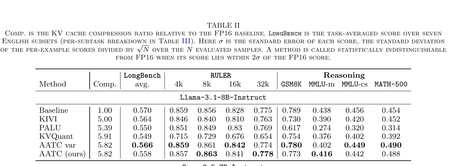
Across all 18 evaluated cells, AATC is never statistically distinguishable from the uncompressed FP16 baseline (within two standard errors). At its main 5.82× operating point (roughly 2.5 bits average per element), AATC reduces Llama’s memory footprint from 1.07 GB to 184 MB. The two backbones respond very differently to compression, which is itself an informative result: on Llama, even the naive scalar baseline KIVI stays near-lossless, and AATC and its var-only ablation are statistically tied throughout — attention-awareness buys nothing extra here because there is little distortion left to be selective about. On Qwen, which the authors identify as markedly harder to compress (KIVI collapses to 0.351 LongBench average and below 0.28 on RULER, versus a 0.574/0.720 FP16 baseline), AATC is the unique best compressed method on long-context retrieval (RULER-32k, +7.2 points over the strongest baseline) and on MMLU-Pro math (+16.8 points). PALU is competitive only at short contexts (best at RULER-4k on Qwen) but posts the weakest LongBench average of any method (0.483), which the paper attributes to its fixed-rank low-rank parameterization losing fine-grained, token-level information that long-range retrieval and exact-match code completion specifically depend on.

6.3 Isolating the benefit of attention-awareness

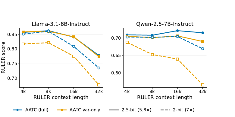
At the main 5.82× operating point, AATC var-only is statistically indistinguishable from full AATC on Llama — which immediately raises the question the authors pose themselves: is the attention-aware weighting actually necessary? Figure 5 answers this by pushing to a more aggressive ≈7× compression (2-bit budget, dashed curves). At 2.5-bit, the two variants are indistinguishable at every context length on Llama. At 2-bit, the full method retains near-baseline RULER accuracy across all context lengths on both models, while the var-only ablation degrades sharply as context grows — most dramatically on Llama at 32k, where var-only falls to roughly 0.68 while full AATC holds near 0.78. This is a clean and honest way to present an ablation: rather than cherry-picking the operating point where your full method looks best, the authors explicitly go looking for the regime where the two variants diverge and report it. The finding itself is intuitive in hindsight: attention-aware weighting matters most exactly when you are compressing aggressively enough that some channels must be sacrificed — the weighting’s whole job is choosing which channels to sacrifice, and that choice is irrelevant when there is enough bit budget for everyone.

6.4 Robustness across bit budgets

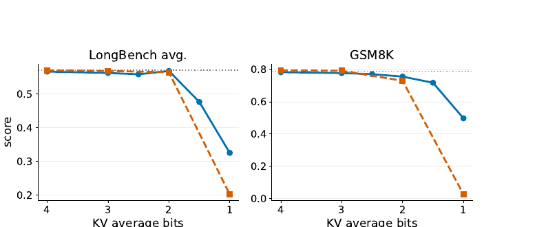
Sweeping the average bit budget from 4 bits down to 1 bit (Figure 6) shows AATC degrading gracefully: LongBench average tracks FP16 within noise from 4-bit down to 2-bit, and GSM8K declines smoothly, with a pronounced drop appearing only at 1.5-bit and below. At the extreme 1-bit setting, AATC remains substantially more robust than KIVI (LongBench 0.33 vs. 0.20; GSM8K 0.50 vs. 0.03) — a large gap that illustrates the practical value of adaptive, transform-and-allocation-based compression once you are past the point where fixed-precision quantization can hold together at all. The paper’s own ablation of the two design axes (allocation strategy versus calibration corpus, run at the 2-bit operating point) attributes most of this robustness to the adaptive allocation itself: replacing it with a single global allocation shared across all channels costs 8.6 LongBench points, and removing just the query-norm term $q_c^2$ costs 3.8 points, while removing the output-projection term $W_{O_c}$ or switching to per-layer allocation costs under 2 points each — a useful signal about which parts of the design carry most of the empirical weight.

7. Reproducibility notes

The paper reports calibration hyperparameters precisely (256 sequences × 2048 tokens, 50/50 FineWeb/OpenR1-Math-220k split, whitening via WikiText-2), the recency-window configuration (first 4 tokens + last 128 tokens in full precision, 16-token refill batches), and the special treatment of the first three transformer layers (given the average value bit-count plus one extra key bit, to compensate for their systematically smaller activation magnitudes). What is not fully specified, and would need to be re-derived or requested from the authors for an exact reproduction: the precise bmax cap used in practice beyond the stated 0–16 range, the exact head-grouping choice rationale for $G=2$ (Llama) versus $G=1$ (Qwen) beyond “matching KV-head count,” and whether the reported KIVI/KVQuant reimplementations (the paper explicitly reimplements both baselines “for fairness” with an added recency window) match the original papers’ reported numbers closely enough to rule out reimplementation-induced gaps — a common and often underspecified risk in any paper that reimplements its own baselines. No training code or public repository is referenced in the version reviewed here, so full numerical reproduction would require re-implementing the whitening-SVD pipeline (Section 5.2) and the reverse-waterfilling solver (Section 5.3) from the equations given, which are precise enough to do so, but non-trivial engineering nonetheless — particularly the per-layer normalization-before-global-allocation step, which is easy to get subtly wrong.

8. Limitations

The authors are candid about several limitations. The cross-token independence assumption in Assumption 1 is explicitly flagged as an idealization: natural language exhibits non-trivial correlation structure between neighboring tokens’ KV representations, and exploiting that correlation would require a computationally intractable token-varying bit allocation — so the paper accepts the idealization as a practical necessity shared by essentially all prior quantization work, rather than claiming it is realistic. On the systems side, the implementation is explicitly not production-optimized: there is no dedicated CUDA kernel, which the authors note would be required before the method could be deployed. The evaluation covers only two model families (Llama and Qwen), and the authors flag that testing on a wider range of architectures — including models with substantially different attention variants beyond grouped-query attention — is left to future work. Finally, the paper notes as open directions both combining AATC with token-eviction methods (recall Section 4’s observation that the token-wise and channel-wise design axes are independent and therefore composable) and extending the per-layer allocation to a global, cross-layer cache as deployed in KVTC.

9. Critical analysis

Weaknesses specific to this paper. First, the headline “no prior method exposes $W_{O_c}$ as an explicit allocation factor” claim, while plausible, rests on a literature survey that the paper itself frames somewhat generously — KVQuant’s Fisher-sensitivity weighting is described as containing $W_O$ only “implicitly, entangled with… the rest of the downstream gradient,” which is true but also somewhat unfalsifiable as a distinguishing claim: any method using an end-to-end loss gradient will have every downstream weight matrix entangled in its sensitivity signal by construction, so the interesting question is whether disentangling $W_{O_c}$ explicitly, as AATC does, produces a measurably different (and better) allocation than the entangled Fisher-sensitivity approach on a head-to-head comparison at matched compression ratios — a comparison the paper does not run directly (KVQuant is compared as a whole pipeline, not isolated on this specific factor). Second, the “AATC var-only is a per-layer analog of KVTC” equivalence claim (Section 5.2, Proposition 1) is a transform-level equivalence, not a full-pipeline equivalence — KVTC operates on a global cross-layer cache with its own allocation criterion, so the empirical comparison in Table II between AATC and KVTC-as-actually-implemented would have been a more direct test of “does per-layer help” than the internal var-only ablation the paper substitutes for it; KVTC does not actually appear in the paper’s main experimental Table II at all, only in the related-work discussion, which is a notable absence given how explicitly the paper positions itself relative to KVTC throughout.

Limitations the authors understate or omit. The paper’s headline claim of being “the first” to expose $W_{O_c}$ and to unify all four channel-level factors is a positioning claim about explicitness, not about final performance — and the ablation in Section 6.4 (removing $W_{O_c}$ costs under 2 LongBench points, versus 8.6 points for removing adaptive allocation entirely) actually shows that $W_{O_c}$, the paper’s most novel individual factor, contributes the least of the ablated components to the measured benchmark scores. The paper reports this number itself but does not foreground the tension between “this is our key theoretical novelty” and “this is the smallest-impact ablation” as clearly as a reader trying to decide which insight to actually adopt in a from-scratch implementation would want. Second, the calibration procedure’s reliance on a specific mixture (FineWeb + OpenR1-Math) means the reported robustness could be partly attributable to the calibration distribution matching the evaluation distribution reasonably well (both contain general text and math reasoning, matching GSM8K/MATH-500/MMLU-Pro-math in the eval suite); the paper’s own calibration ablation shows GSM8K “is not affected by any variant” of the calibration mix, which is reassuring, but a fully out-of-domain calibration test (e.g., calibrating only on code and evaluating on math) is not reported and would more directly stress-test the claim that the method generalizes beyond its calibration distribution.

Concrete improvement suggestions. (1) Report a direct head-to-head comparison against the actual KVTC pipeline (not just the internal var-only proxy) at matched compression ratios on both backbones, to validate the claimed per-layer-vs-global-transform advantage empirically rather than by equivalence proof plus proxy ablation. (2) Run the joint-key-value-budget ablation explicitly (a single reverse-waterfilling pool across both keys and values, with appropriate weight normalization) to justify the separate-budgets design choice with data rather than architectural reasoning alone. (3) Add a genuinely out-of-domain calibration robustness test — calibrate on one domain (e.g., code, or a single language) and evaluate on a disjoint domain (e.g., long-document QA in another language, or math) — to bound how much of the near-lossless result depends on calibration-eval distributional overlap, since the current calibration mixture and evaluation suite share substantial domain overlap. (4) Provide the promised CUDA kernel or at least a wall-clock latency/throughput measurement under a real serving stack (vLLM-style batched decoding), since without it the 5.8× memory compression claim cannot yet be translated into a corresponding claim about serving throughput or latency, which is ultimately what KV cache compression is deployed to improve.

10. Conclusion

AATC’s contribution is best understood as a derivation, not an invention: the transform-coding and reverse-waterfilling machinery is decades old, and per-channel bit allocation for KV caches already existed in KVTC. What AATC adds is a rigorous, closed-form answer to the question “allocate bits against what, exactly?” — proving that the attention-output distortion, under the standard white-noise quantization model, decomposes additively into key and value terms that each factor cleanly into a token-dependent and a channel-dependent piece. That decomposition is genuinely useful independent of AATC’s specific algorithm: it gives the field a common mathematical language (Table I’s five factors) for comparing eviction methods, rotation methods, and quantization methods that previously looked like unrelated tricks. The algorithm built on top of the decomposition is a fairly direct, calibration-cheap application of reverse waterfilling to the newly-derived weighted variance — no learned components, no exotic codebooks — which is a genuine strength for deployability once a production kernel exists, and the empirical story (near-lossless at 5.8×, meaningfully more robust than fixed-precision baselines at 7× and below) is honestly reported, including the ablation that shows attention-awareness matters most exactly where you would predict it to: in the aggressive-compression, long-context regime where every bit is contested.