GCPO: Why Some GRPO Updates Quietly Break Your Model, and How to Structurally Forbid Them

Review date: 2026-08-18 Author: Zhongzhu Zhou Paper reviewed: GCPO: Diagnosing and Constraining Subspace Geometry in Rollout RL for LLMs Paper authors: Kai Yang, Jingwei Xu, Wanyu Wang, Kai-Yuan Guo, Zhenbo Yu, Yi Wang, Yu Qiao (Shanghai Jiao Tong University; Shanghai AI Laboratory; NovaCore; Huazhong University of Science and Technology) arXiv: 2608.11674 Venue/Status: arXiv preprint, August 2026

1. The problem: RL post-training destabilizes itself, and nobody can quite say why

If you’ve run GRPO, DAPO, GSPO, or any other rollout-based RL post-training recipe on an LLM at scale, you’ve probably seen at least one of these three symptoms: accuracy that oscillates wildly instead of climbing smoothly, a model that gets great at the task you’re training on but visibly worse at everything else, or a policy that learns to pad its answers with useless tokens because longer responses happen to correlate with higher reward. None of these are new observations — they’re folklore-level common knowledge in the RLHF/RLVR community. What’s been missing is a mechanistic account of where these failures come from at the level of the actual parameter updates, as opposed to symptom-level explanations (“the KL penalty was too weak,” “the clipping range was wrong,” “reward hacking”).

This paper’s contribution is to open that black box using tools from numerical linear algebra rather than RL theory. The authors ask a very specific, almost mundane-sounding question: when a rollout-based RL algorithm updates a weight matrix, how does that update’s direction relate to the pretrained weight matrix’s own dominant singular directions? And they find something that is not mundane at all: transient spikes in this overlap — moments where the RL update briefly aligns itself with the pretrained model’s most “load-bearing” directions — reliably precede performance degradation. From that diagnosis, they build GCPO (Geometrically Constrained Policy Optimization), which doesn’t try to discourage this behavior with a penalty term (which, as we’ll see, quietly fails), but instead makes it structurally impossible through a clever reparameterization of the trainable update.

This review works through the linear-algebra machinery in full — the four-way decomposition of an update, the dimension correction that makes the overlap statistic meaningful, the controlled intervention experiment that turns correlation into evidence of causation — then unpacks the GCPO parameterization itself, walks through the full experimental picture (six benchmark settings, cross-task transfer, training dynamics, four separate ablation axes), and closes with a critical look at what’s still missing.

One framing worth keeping in mind throughout: this paper is doing two logically separable things at once, and it’s worth tracking them as distinct threads. The first is a measurement contribution — a way to quantify, cheaply and with a principled statistical baseline, how much any given parameter update touches a pretrained model’s structurally dominant directions. The second is a design contribution — a specific way to use that measurement to build a training-time constraint. You could in principle accept the first without accepting the second (maybe you’d rather use the overlap statistic purely as a monitoring dashboard and intervene manually, or with a different mechanism than a hard reparameterization), and you could imagine building other fixes on top of the same diagnostic. Keeping these two contributions distinct helps when evaluating the paper’s evidence: the diagnostic claim (Section 3) needs to survive scrutiny about correlation-versus-causation, while the design claim (Section 4–5) needs to survive scrutiny about whether GCPO is actually the best way to act on that diagnosis, or merely a reasonable one.

2. Prerequisites: what you need going in

Rollout-based RL for LLMs, briefly. In RLHF/RLVR-style post-training, a policy $\pi_\theta$ generates multiple candidate responses (“rollouts”) per prompt, each response gets a scalar reward (from a learned reward model, a rule-based verifier, or execution feedback), and the policy is updated to increase the probability of high-reward rollouts relative to low-reward ones. GRPO (Group Relative Policy Optimization) is the dominant recipe in this space: instead of training a separate value function/critic to estimate a baseline (as classic PPO does), GRPO samples $K$ rollouts per prompt and uses the within-group mean reward as the baseline, turning the advantage of each rollout into a simple standardized z-score relative to its siblings. This is cheap (no critic network) and works well in practice, but the updates it produces are still generated by a moving target: each gradient step changes the policy, which changes the next batch of rollouts, which changes the next gradient step. This is a feedback loop, and feedback loops are exactly the kind of system that can develop instabilities that a naive first-order analysis misses.

GSPO, DAPO, and GMPO are all variants that modify some piece of this recipe — the level at which importance-ratio clipping is applied (token vs. sequence), the way outlier or degenerate groups are filtered, or the choice of geometric vs. arithmetic mean when aggregating token-level ratios — while keeping the same overall group-relative-advantage skeleton. All four of these serve as baselines in this paper’s experiments, and it’s worth being specific about what each one changes, since the paper leans on them as a representative slice of “the current state of the art in objective-level fixes,” and the comparison against them is only as informative as the reader’s understanding of what they actually do differently. GSPO (Group Sequence Policy Optimization) applies the importance-ratio clipping at the sequence level rather than per-token, on the reasoning that per-token ratios in a long generated sequence can vary wildly even when the sequence as a whole is a reasonable update, and this sequence-level view tends to reduce a specific kind of gradient-variance blow-up. DAPO (Decoupled Clip and Dynamic Sampling Policy Optimization) decouples the upper and lower clipping thresholds (rather than using one symmetric range) and dynamically filters out prompts whose entire rollout group has degenerate advantages (all-correct or all-incorrect groups, which otherwise contribute zero learning signal but still cost compute), which tends to make training more sample-efficient per prompt but can also, as this paper’s Figure 5 result suggests, tolerate more exploratory (and longer) rollouts along the way. GMPO (Geometric-Mean Policy Optimization) replaces the arithmetic mean used to aggregate per-token importance ratios within a sequence with a geometric mean, which is less sensitive to a small number of individual tokens with extreme ratios dominating the aggregate signal. None of these four baselines touches the parameter-space direction of the resulting update at all — they all operate purely on how the objective function’s scalar value is computed from the rollouts, which is exactly the gap GCPO is designed to fill, and is why it’s a fair and informative comparison rather than an apples-to-oranges one: GCPO is compatible with, not competing against, any of these four objective-level choices, since it constrains the update parameterization while leaving the loss computation itself untouched.

Singular Value Decomposition (SVD) as a lens on a weight matrix. Any real matrix $W_{\text{ref}} \in \mathbb{R}^{d_{\text{out}} \times d_{\text{in}}}$ can be written as $W_{\text{ref}} = \Phi \Sigma \Psi^\top$, where $\Phi$ and $\Psi$ are orthogonal matrices (their columns are the left and right singular vectors) and $\Sigma$ is diagonal with non-negative entries sorted in decreasing order. The columns of $\Psi$ corresponding to the largest singular values span the directions in the input space that this matrix responds most strongly to; the columns of $\Phi$ corresponding to the largest singular values span the directions in the output space that the matrix writes into most strongly. If you truncate to the top $k$ singular vectors on each side, $\Phi_k \Sigma_k \Psi_k^\top$ is the best possible rank-$k$ approximation of $W_{\text{ref}}$ in Frobenius norm — this is the classical Eckart–Young–Mirsky theorem. This paper calls $\text{span}(\Phi_k)$ and $\text{span}(\Psi_k)$ the principal subspaces of a pretrained weight matrix: not because they represent literal, interpretable “concepts,” but because they are the structurally dominant components of that matrix’s linear behavior, in a way that is cheap to compute (one SVD, done once, before training starts) and easy to reason about geometrically.

Frobenius inner product and orthogonal projectors. For two matrices $A, B$ of the same shape, their Frobenius inner product is $\langle A, B \rangle_F = \text{tr}(A^\top B)$, and $\|A\|_F^2 = \langle A, A \rangle_F$ is just the sum of squared entries — the natural notion of “energy” for a matrix update. Given an orthonormal basis $\Phi_k$ for a $k$-dimensional subspace, $\Pi_\Phi = \Phi_k \Phi_k^\top$ is the orthogonal projector onto that subspace (applying it to any vector gives the closest point in the subspace), and $\Pi_\Phi^\perp = I - \Pi_\Phi$ projects onto the orthogonal complement. These two projectors are idempotent ($\Pi_\Phi^2 = \Pi_\Phi$) and mutually annihilating ($\Pi_\Phi \Pi_\Phi^\perp = 0$), which is the algebraic fact that makes the four-way energy decomposition in the next section exact rather than approximate.

LoRA, briefly, for contrast. Low-Rank Adaptation (LoRA) replaces a full-rank weight update $\Delta W$ with a low-rank product $\Delta W = BA$ where $B \in \mathbb{R}^{d_{\text{out}} \times r}$, $A \in \mathbb{R}^{r \times d_{\text{in}}}$, and $r \ll \min(d_{\text{out}}, d_{\text{in}})$. This is primarily a parameter-efficiency trick: it reduces the number of trainable parameters and the associated optimizer state, but it does not, by itself, constrain which directions in the full $d_{\text{out}} \times d_{\text{in}}$ space the update can point in — a rank-$r$ update parameterized this way can still, over the course of training, drift toward any direction, including the pretrained model’s principal subspaces. This distinction — low rank as compression versus low rank as a vehicle for an exact directional constraint — is the crux of how GCPO differs from plain LoRA fine-tuning under an RL objective, and the paper takes care to isolate the two effects experimentally (more on this in Section 6).

3. The diagnostic: decomposing an update into four geometric blocks

3.1 The four-way split

The object of interest is not the raw gradient but the realized update at optimization step $t$:

$$\delta^{(t)} W = W_t - W_{t-1}.$$

This choice matters: the realized update already has the optimizer’s learning rate, momentum, and (for AdamW) per-coordinate adaptive scaling baked into it, so this analysis is measuring what actually happened to the weights, not an idealized gradient direction.

Given the principal-subspace projectors $\Pi_\Phi, \Pi_\Psi$ (built from the pretrained weight’s top-$k$ singular vectors) and their complements $\Pi_\Phi^\perp, \Pi_\Psi^\perp$, any update can be split into four mutually orthogonal blocks by projecting each side (left/output, right/input) onto either the principal subspace or its complement:

$$\delta^{(t)} W = \underbrace{\Pi_\Phi \delta^{(t)} W \Pi_\Psi}_{\delta^{(t)} W^{PP}} + \underbrace{\Pi_\Phi \delta^{(t)} W \Pi_\Psi^\perp}_{\delta^{(t)} W^{PO}} + \underbrace{\Pi_\Phi^\perp \delta^{(t)} W \Pi_\Psi}_{\delta^{(t)} W^{OP}} + \underbrace{\Pi_\Phi^\perp \delta^{(t)} W \Pi_\Psi^\perp}_{\delta^{(t)} W^{OO}}. \tag{1}$$

Read the superscripts as (output-side, input-side): $PP$ means the update writes into a principal output direction and reads from a principal input direction; $OO$ means it avoids both. Because $\Pi_\Phi \Pi_\Phi^\perp = 0$ and $\Pi_\Psi \Pi_\Psi^\perp = 0$, these four blocks are pairwise orthogonal under the Frobenius inner product — you can check this directly: the inner product of the $PP$ and $PO$ blocks is $\text{tr}(\Pi_\Psi \delta^{(t)}W^\top \Pi_\Phi \delta^{(t)}W \Pi_\Psi^\perp)$, and cyclic invariance of the trace plus $\Pi_\Psi^\perp \Pi_\Psi = 0$ collapses this to zero, and the same argument goes through for every other cross-term. This orthogonality is what makes the following energy decomposition exact (a Pythagorean-style identity) rather than an approximation:

$$\|\delta^{(t)} W\|_F^2 = E_{PP} + E_{PO} + E_{OP} + E_{OO}, \qquad E_{ij} = \|\delta^{(t)} W^{ij}\|_F^2. \tag{9}$$

The headline overlap statistic is then just the fraction of update energy that touches the principal subspace on at least one side:

$$O_t = \frac{E_{PP} + E_{PO} + E_{OP}}{E_{\text{total}}} = 1 - \frac{E_{OO}}{E_{\text{total}}}. \tag{2}$$

3.2 Why you need a dimension correction

Here’s the subtlety that makes this measurement non-trivial: even a completely random, isotropically-directed update has nonzero expected overlap with any fixed $k$-dimensional subspace, simply because that subspace has positive dimension. If you don’t correct for this, you can’t tell whether an observed $O_t$ reflects a genuine directional preference or just the baseline geometric fact that $k > 0$.

The paper derives the exact correction. Vectorize the update, $z = \text{vec}(\delta W) \in \mathbb{R}^D$ with $D = d_{\text{out}} d_{\text{in}}$. The doubly-orthogonal component can be written as a single linear projection $Qz$ where $Q = \Pi_\Psi^\perp \otimes \Pi_\Phi^\perp$ (using the vectorization identity for Kronecker products), and $Q$ is itself an orthogonal projector with rank $(d_{\text{out}} - k)(d_{\text{in}} - k)$ — the product of the two complement dimensions. For a uniformly random direction $z / \|z\|_2$ on the unit sphere in $\mathbb{R}^D$, a standard fact about isotropic random vectors gives $\mathbb{E}[zz^\top / \|z\|_2^2] = I_D / D$, and therefore

$$\mathbb{E}\left[\frac{\|Qz\|_2^2}{\|z\|_2^2}\right] = \text{tr}\left(Q \, \mathbb{E}\left[\frac{zz^\top}{\|z\|_2^2}\right]\right) = \frac{\text{rank}(Q)}{D} = \frac{(d_{\text{out}} - k)(d_{\text{in}} - k)}{d_{\text{out}} d_{\text{in}}}. \tag{18-20}$$

Since the overlap statistic is $O = 1 - \|Qz\|_2^2 / \|z\|_2^2$ (the fraction of energy not in the doubly-orthogonal block), this immediately gives the null value:

$$O_{\text{null}} = 1 - \frac{(d_{\text{out}} - k)(d_{\text{in}} - k)}{d_{\text{out}} d_{\text{in}}}. \tag{3}$$

The reported quantity is then the excess overlap relative to this null:

$$O_t^{\text{excess}} = O_t - O_{\text{null}}. \tag{4}$$

A positive $O_t^{\text{excess}}$ means the update is more aligned with the principal subspaces than an isotropic update of the same size would be by chance — a genuine directional signal, not a dimensionality artifact.

A concrete number helps ground this. Take a Qwen3-8B attention projection matrix with, say, $d_{\text{out}} = d_{\text{in}} = 4096$ and a protected rank of $k=8$ (the value the ablation in Section 5.5 finds is optimal). Plugging into Equation 3:

$$O_{\text{null}} = 1 - \frac{(4096-8)(4096-8)}{4096 \times 4096} = 1 - \frac{4088^2}{4096^2} \approx 1 - 0.9961 = 0.0039.$$

So a purely random update direction would, by chance alone, already show about 0.39% overlap with an 8-dimensional principal subspace in a 4096-dimensional matrix — small, but not zero, and this is exactly the baseline that has to be subtracted out before any observed overlap can be interpreted as a genuine directional preference. Figure 1’s reported excess-overlap values (on the order of 0.03–0.05 for Qwen3-8B, 0.0135–0.018 for GLM4-9B) are roughly one to two orders of magnitude larger than this null value, which is a useful sanity check that the observed spikes are not simply an artifact of this dimension-correction baseline creeping upward. This is a clean and important piece of statistical hygiene: without it, you’d be tempted to read meaning into overlap numbers that are actually just baseline noise from working in a subspace of positive dimension, and this is exactly the kind of subtlety that’s easy to skip if you only read the headline plot and not the appendix proof.

3.3 What the data shows

Figure 1 (reproduced below) plots this excess overlap over training steps for Qwen3-8B on GSM8K and GLM4-9B on MATH500, alongside held-out validation accuracy.

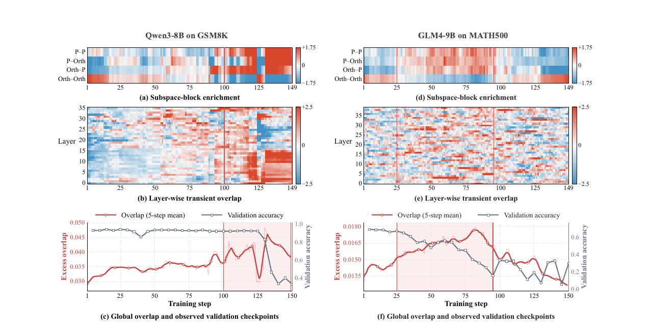
Two findings stand out. First, on aggregate, the vast majority of update energy does sit in the doubly-orthogonal ($OO$) block — 93.8% for Qwen3-8B and 97.7% for GLM4-9B, on average — which is consistent with prior work’s finding that RL updates are, in the long run, predominantly off-principal. Second, and this is the paper’s actual empirical contribution, this aggregate statistic hides the interesting behavior: there are sustained or repeated spikes in excess overlap, and these spikes reliably precede validation-accuracy degradation, sometimes as a gradual decline and sometimes as a sharp drop. The layer-wise panels (b)/(e) further show that these spikes are not diffuse across all layers — they concentrate in specific, often intermediate-to-upper, layers, which is itself informative: it suggests the instability has a localized mechanistic origin rather than being a global drift.

It’s worth being precise about what this figure does and doesn’t establish. The paper is explicit that this is a correlational observation — elevated overlap and subsequent degradation co-occur and the former precedes the latter in time, but temporal precedence alone doesn’t rule out a shared underlying cause (e.g., some other training pathology that both elevates overlap and independently degrades performance a few steps later). That’s exactly why the next experiment matters.

3.4 The controlled intervention: turning correlation into evidence

To get closer to a causal claim, the authors take a single GRPO update (step 150, Qwen3-8B on ToolAlpaca), and directly manipulate its principal-overlapping component by a scaling factor $\eta$, while holding the Frobenius norm of each layer’s update fixed (so any accuracy change can’t just be attributed to the update having gotten bigger or smaller overall). At $\eta = 1$ you recover the original update (56.89% accuracy in this slice); $\eta = 0$ removes the principal-overlapping component entirely (orthogonalizing the update); $\eta > 1$ injects more principal-subspace alignment than was originally there.

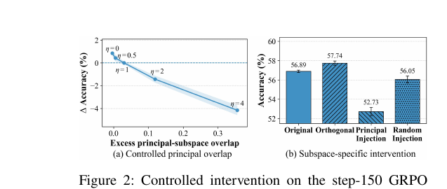
The result is about as clean as controlled interventions on live-trained LLM checkpoints get: accuracy falls monotonically and substantially as $\eta$ increases (a clear dose-response curve), removing the overlap ($\eta=0$) improves accuracy relative to the original update, and — crucially for ruling out a magnitude-only explanation — injecting the same amount of extra energy into a random subspace of matched dimension causes far less damage than injecting it into the principal subspace specifically. This is the piece of evidence that moves the paper from “here’s an interesting correlation” to “here’s a mechanism we have reason to believe is causally implicated,” and it’s the direct empirical justification for why GCPO’s design targets direction rather than, say, just adding more gradient clipping or a bigger KL penalty (which would only control magnitude/divergence, not direction).

4. The fix: GCPO’s projected low-rank parameterization

4.1 Problem formulation

Given the diagnosis, the natural next step is to ask: rather than just discouraging principal-subspace overlap with a penalty (soft), can we make it impossible by construction (hard)? The paper formulates this as a constrained variant of the usual RL objective. Let $\theta_0$ be the pretrained policy, $M$ the set of adapted linear layers, and $\Delta\theta$ the trainable update. The constrained problem is:

$$\max_{\Delta\theta} \; J_{\text{rollout}}(\pi_{\theta_0 + \Delta\theta}) - \beta D_{\text{KL}}(\pi_{\theta_0+\Delta\theta} \,\|\, \pi_{\text{ref}}) \tag{5}$$ $$\text{s.t.} \quad \Phi_k^{(\ell)\top} \delta^{(t)} W^{(\ell)} = 0, \qquad \delta^{(t)} W^{(\ell)} \Psi_k^{(\ell)} = 0, \quad \forall \ell \in M. \tag{6, 7}$$

The two constraints together say exactly “retain only the $OO$ block at every layer, every step” — zero overlap with the principal subspace on either side, for every single realized update, not just on average. Note this is explicitly framed as complementary to, not a replacement for, KL regularization: KL controls how much the policy’s output distribution is allowed to move; the new constraint controls which directions in parameter space the update is allowed to move in. You could, in principle, have a small-KL update that’s still concentrated in the dangerous principal directions, or a large-KL update that’s entirely off-principal — these are genuinely different axes of control.

The paper is candid that a soft version of this — adding a penalty term like $\|\Phi_k^\top \delta W\|_F^2 + \|\delta W \Psi_k\|_F^2$ to the loss — was tried and considered as the obvious first move, but it underperforms (Table 3, discussed in Section 6). The reasoning given is that under the iterative feedback loop of RL — where each update changes the rollout distribution that generates the next update’s gradient — a soft penalty is just one term competing against the (often much larger and more variable) task-reward gradient, and dominant task gradients can and do overwhelm it over the course of training. A hard constraint doesn’t have this failure mode because it isn’t a trade-off at all; it’s a change to what’s representable.

4.2 The parameterization that makes the constraint free

Here is the key design trick, and it’s elegant enough to be worth walking through slowly. For each adapted layer, with the projectors $\Pi_\Phi^\perp, \Pi_\Psi^\perp$ fixed once (computed from the pretrained weight’s SVD, before training starts), parameterize the layer’s update as:

$$\delta^{(t)} W^{(\ell)} = \alpha \, \Pi_\Phi^{\perp(\ell)} L^{(\ell)} R^{(\ell)} \Pi_\Psi^{\perp(\ell)}, \tag{8}$$

where $L^{(\ell)}$ and $R^{(\ell)}$ are ordinary trainable low-rank factors (shape $d_{\text{out}} \times r$ and $r \times d_{\text{in}}$, just like LoRA) and $\alpha$ is a fixed scaling constant. The trick is that the projectors are applied on the outside of the trainable factors, sandwiching them. Because $\Pi_\Phi^{\perp}$ and $\Pi_\Psi^{\perp}$ are themselves fixed (not trained), no matter what values the trainable factors $L, R$ take during optimization, the resulting update is already guaranteed to satisfy both constraints — you can verify this directly: left-multiplying by $\Phi_k^\top$ gives $\Phi_k^\top \Pi_\Phi^\perp (\cdot) = 0$ because $\Phi_k^\top \Pi_\Phi^\perp = 0$ by definition of the complement projector, and the symmetric argument holds on the right side with $\Psi_k$.

This is the central move of the paper: it converts a constraint that would otherwise need to be enforced, checked, or penalized during optimization into a structural property of the parameterization itself. The optimizer never sees the constraint as a constraint — it just does ordinary unconstrained gradient descent on $L$ and $R$, and the projectors silently absorb any gradient signal that would have pushed the effective update toward the principal subspace, because that component gets annihilated by $\Pi_\Phi^\perp (\cdot) \Pi_\Psi^\perp$ regardless of what $L, R$ contain. This is analogous in spirit to how you’d enforce a linear equality constraint in classical optimization by reparameterizing the feasible set rather than adding a Lagrange multiplier — except here it’s being applied inside a deep, iteratively-retrained RL loop where a soft Lagrangian approach demonstrably fails (Section 4.1).

4.3 Algorithm, step by step

Algorithm 1 in the paper lays out the full training loop; here it is unpacked into prose alongside the pseudocode.

Setup (once, before training):

1. For each adapted layer $\ell \in M$, compute the top-$k$ singular vectors $\Phi_k^{(\ell)}, \Psi_k^{(\ell)}$ of the pretrained weight $W_{\text{ref}}^{(\ell)}$. This is a single SVD per layer, done once — no repeated cost during training.
2. Initialize the trainable factor $L^{(\ell)}$ to zero and $R^{(\ell)}$ with the standard LoRA initialization (typically small random values), matching the usual LoRA convention that the adapter starts as a no-op ($LR = 0$ at step 0, so the model starts exactly at the pretrained weights).

Each training step $t = 1, \dots, T$, for each adapted layer $\ell$:

1. Project the raw trainable factors onto the complement subspace: $\bar{L}^{(\ell)} \leftarrow L^{(\ell)} - \Phi_k^{(\ell)} (\Phi_k^{(\ell)\top} L^{(\ell)})$ and $\bar{R}^{(\ell)} \leftarrow R^{(\ell)} - (R^{(\ell)} \Psi_k^{(\ell)}) \Psi_k^{(\ell)\top}$. This is exactly the projector applied to $L$ and $R$ before they’re multiplied together and injected into the layer, which is algebraically equivalent to applying $\Pi_\Phi^\perp(\cdot)\Pi_\Psi^\perp$ to the product but cheaper to compute (you project two thin matrices instead of one dense one).
2. Form the effective weight for this step: $W_t^{(\ell)} \leftarrow W_{\text{ref}}^{(\ell)} + s \bar{L}^{(\ell)} \bar{R}^{(\ell)}$, where $s = \alpha / r$ is the standard LoRA scaling constant.
3. Synchronize these projected weights out to the rollout-generation engine (e.g., vLLM), since rollouts must be generated from the actual current policy, projections included.
4. Generate rollouts under this policy, compute the usual GRPO-style policy-optimization loss on them.
5. Backpropagate and update the raw, unprojected factors $L^{(\ell)}, R^{(\ell)}$ with the optimizer (AdamW). Note that gradients flow back through the projection step, so the optimizer does see gradients on the raw factors that reflect the projected forward pass — but the projection is reapplied fresh at the start of every step, so drift of the raw factors into the principal subspace has literally zero effect on the model’s behavior; it’s invisible, wasted capacity, not a constraint violation waiting to happen.

The cost overhead relative to plain LoRA is genuinely small: two extra small matrix projections per adapted layer per step (each roughly $O(d \cdot k \cdot r)$, cheap because $k$ and $r$ are both small relative to $d$), plus one SVD per layer computed once up front. The paper reports that GCPO’s peak GPU memory is essentially identical to plain LoRA (Figure 6, discussed in Section 5), which makes sense since the trainable parameter count and optimizer state are unchanged — the only addition is a small amount of extra compute per forward pass, not extra state.

To make this concrete: with $d = 4096$, $k=8$, and $r=32$ (the main-experiment configuration), each of the two projection steps costs roughly $4096 \times 8 \times 32 \approx 1.05\text{M}$ multiply-adds — negligible next to the $4096 \times 4096 \times 32 \approx 537\text{M}$ multiply-adds of the low-rank matrix product $\bar{L}\bar{R}$ itself, which is the same cost plain LoRA already pays. The one-time SVD cost (computing the top-$k$ singular vectors of every adapted weight matrix, once, before training starts) is likewise small in the grand scheme: a randomized/truncated SVD for $k=8$ on a $4096\times4096$ matrix is far cheaper than a full SVD and takes a small fraction of a single training step’s wall-clock time, amortized over the hundreds of steps in a full RL run.

4.4 Why this actually preserves the pretrained mapping (not just “on average”)

The paper proves a genuinely strong guarantee, not just an average-case argument. Because the cumulative adaptation $\Delta W_t^{(\ell)} = W_t^{(\ell)} - W_{\text{ref}}^{(\ell)}$ has the same sandwiched-projector form at every step (it’s a sum of terms that all individually satisfy the constraint, and the constraint is linear, so the sum does too), you get a clean corollary: for any input $x$ lying exactly in the principal input subspace ($x \in \text{span}(\Psi_k^{(\ell)})$), the adapted layer’s output is identical to the pretrained layer’s output, $W_t^{(\ell)} x = W_{\text{ref}}^{(\ell)} x$ — not approximately preserved, exactly preserved, at every single training step, not just at convergence. The symmetric statement holds for the output side: for any $y$ in the principal output subspace, $y^\top W_t^{(\ell)} = y^\top W_{\text{ref}}^{(\ell)}$.

This is a genuinely useful, checkable, layer-local property — but it’s worth being precise about its scope, and this is one place I think the paper could be more careful in how it’s presented. The guarantee is about a specific linear layer’s response to inputs in a specific subspace; it is explicitly not a claim that any particular semantic capability of the model — factual knowledge, a skill, a behavior — lives in that subspace and is therefore protected. The paper itself flags this (“we treat them as a functionally distinguished yet tractable structural reference,” not “a literal decomposition of semantic knowledge”), and the algebraic Corollary B.4 explicitly says the same: it’s a per-layer, per-subspace input/output guarantee, not a model-level capability-preservation guarantee. The empirical capability-retention results in Section 5.2 are consistent with the hypothesis that protecting these directions helps preserve general capability, but they are a separate, correlational, empirical finding layered on top of an unrelated exact algebraic fact about one linear map. Conflating the two — treating the exact per-layer guarantee as if it directly implied the empirical capability-retention result — would be a mistake, and a careful reader should keep them separate even though the paper’s narrative flow invites blurring them together.

4.5 How GCPO differs from LoRA-style continual-learning constraints

There’s a family of prior work (the paper cites GeoLoRA, MiLoRA, and orthogonal-subspace continual learning) that also uses subspace geometry to prevent catastrophic forgetting during supervised fine-tuning — restricting updates away from directions important for previously-learned tasks. GCPO’s motivation is different in an important way: those methods are designed for a largely static data distribution (fixed fine-tuning data, sequential tasks), where the concern is forgetting task A while learning task B. GCPO’s target failure mode is a dynamical one specific to on-policy RL: rollouts are generated by the current policy, so every update changes the distribution that produces the next update’s training signal, and it’s specifically this feedback loop that the paper’s diagnostic work (Section 3) shows produces transient — not sustained — principal-subspace excursions. This is why a hard, always-on constraint (rather than a penalty that could in principle be relaxed once training stabilizes) is the design choice: you can’t easily predict when the next transient spike will occur, so the constraint needs to be unconditionally active throughout training.

5. Experiments: does it actually work, and does it work for the claimed reasons?

5.1 Setup

The evaluation uses two backbones — Qwen3-8B and GLM4-9B — across three task domains chosen to span distinct reward structures: mathematical reasoning on MATH500 (reward = exact match on the final boxed answer via rule-based parsing), code generation on HumanEval+ (reward = fraction of unit tests passed), and tool use on ToolAlpaca (reward = a composite of function-name match, argument-key consistency, and normalized argument-value matching). All three use binary or graded response-level rewards, no learned reward model. Held-out splits are fixed across all methods (seed 42), and every training configuration is repeated over three independent seeds, with results reported as mean $\pm$ standard deviation. Evaluation uses majority@16 accuracy (16 sampled responses per test example, majority vote, then bootstrap-estimated over 1,000 resamples) — a reasonably robust choice that reduces sensitivity to any single unlucky sample.

GCPO is compared against a genuinely comprehensive baseline suite: vanilla GRPO; three objective-level variants that modify the clipping/aggregation scheme (GSPO, DAPO, GMPO); and — critically for isolating GCPO’s actual contribution — GRPO-LoRA, which uses the exact same rank and scaling as GCPO but without the bilateral orthogonality constraint. This last baseline is the one that matters most for a clean causal story: if GCPO merely outperformed full-parameter GRPO, a skeptic could reasonably attribute the gain to low-rank regularization alone (a well-known implicit regularizer in fine-tuning). Comparing directly against GRPO-LoRA at matched rank isolates the orthogonal projection itself as the source of any additional gain.

The adapted rank is $r=32$ with $\alpha=16$ for both LoRA and GCPO, and the protected principal rank is $k=8$, chosen by the ablation in Section 5.4 below. Training runs for up to 300 steps with a rollout group size of $K=16$; full hyperparameters (learning rates per method, clipping thresholds, batch sizes) are in the paper’s Appendix D and are held consistent across methods for a fair comparison.

5.2 Main accuracy results: GCPO wins everywhere, with the tightest variance

Method	MATH500	HumanEval+	ToolAlpaca
Qwen3-8B
Base (Instruct)	67.46	73.58	56.53
GRPO	72.00 ± 1.36	84.24 ± 0.88	59.56 ± 1.52
GSPO	77.80 ± 0.74	87.81 ± 0.51	66.18 ± 0.82
DAPO	78.33 ± 0.61	88.13 ± 0.48	65.99 ± 0.76
GMPO	77.64 ± 0.69	88.14 ± 0.45	66.16 ± 0.71
GRPO-LoRA	77.87 ± 0.58	87.36 ± 0.62	66.05 ± 0.67
GCPO	79.47 ± 0.31	89.16 ± 0.27	67.26 ± 0.39
GLM4-9B
Base (Instruct)	66.51	76.55	42.47
GRPO	59.43 ± 1.84	72.43 ± 1.42	65.70 ± 1.65
GSPO	71.29 ± 0.97	79.55 ± 0.83	66.22 ± 1.08
DAPO	72.41 ± 0.82	81.43 ± 0.71	67.35 ± 0.93
GMPO	71.33 ± 0.91	80.63 ± 0.76	67.79 ± 0.88
GRPO-LoRA	72.34 ± 0.66	81.48 ± 0.59	66.19 ± 0.75
GCPO	74.56 ± 0.34	83.64 ± 0.29	70.16 ± 0.41

GCPO achieves the best accuracy in all six model-task combinations, beating the strongest competing baseline in each cell by 1.02–2.37 points, and — notably — has the lowest standard deviation in every single setting. That last detail is easy to skim past but is arguably as important as the mean improvement: a hard geometric constraint that also reduces run-to-run variance is doing something structurally different from a method that just happens to find a slightly better optimum on average. It’s consistent with the training-stability story in Section 5.3 below — a training process with fewer destabilizing excursions should also be a more reproducible one across random seeds.

The comparison against GRPO-LoRA specifically confirms the paper’s causal claim: at matched rank, GCPO beats GRPO-LoRA in every one of the six settings, which means the orthogonal projection is contributing something beyond what low-rank parameterization alone provides. This is exactly the ablation you’d want to see, and its inclusion strengthens the paper’s central claim considerably.

5.3 Cross-task capability retention: the ToolAlpaca collapse

A single-domain RL run is only useful if it doesn’t wreck the model’s other capabilities. The authors post-train on MATH500 only, then evaluate on HumanEval+ and ToolAlpaca — tasks the model was never trained on in this run.

Method	HumanEval+ (Δ)	ToolAlpaca (Δ)	Worst Δ
Qwen3-8B, base: 73.58 / 56.53
GRPO	64.71 (−8.87)	50.72 (−5.81)	−8.87
GSPO	76.82 (+3.24)	53.41 (−3.12)	−3.12
DAPO	75.54 (+1.96)	53.09 (−3.44)	−3.44
GMPO	74.31 (+0.73)	52.90 (−3.63)	−3.63
GRPO-LoRA	74.63 (+1.05)	56.69 (+0.16)	+0.16
GCPO	77.57 (+3.99)	57.56 (+1.03)	+1.03
GLM4-9B, base: 76.55 / 42.47
GRPO	76.91 (+0.36)	27.50 (−14.97)	−14.97
GSPO	81.58 (+5.03)	41.29 (−1.18)	−1.18
DAPO	81.39 (+4.84)	37.68 (−4.79)	−4.79
GMPO	79.76 (+3.21)	41.33 (−1.14)	−1.14
GRPO-LoRA	81.00 (+4.45)	43.14 (+0.67)	+0.67
GCPO	82.43 (+5.88)	43.38 (+0.91)	+0.91

The headline number here is GRPO’s catastrophic ToolAlpaca collapse on GLM4-9B: training on math alone drops tool-use accuracy by nearly 15 points (from 42.47 to 27.50). This is a striking illustration of the “forgetting” problem RL post-training can inflict on capabilities orthogonal to the training task, and every objective-level baseline (GSPO, DAPO, GMPO) also shows a real ToolAlpaca regression, just a smaller one — suggesting that clipping/aggregation-level fixes alone don’t address the underlying parameter-space cause. GCPO and (to a lesser extent) plain GRPO-LoRA are the only methods that actually improve ToolAlpaca relative to the base model while training exclusively on math, and GCPO has the best worst-case retention on both backbones. Interestingly, math-to-code transfer is mostly positive for every method (both tasks reward step-by-step symbolic reasoning), which is a useful reminder that “cross-task degradation” is not uniform — it depends on how related the held-out task’s underlying skill is to the trained task’s skill, and tool-calling (a much more format- and precision-sensitive skill) appears to be the more fragile capability here.

5.4 Training dynamics: stability, entropy, and length control

Three separate dynamical properties are examined, and all three point the same direction.

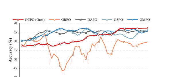
Training stability. GRPO’s accuracy trajectory on ToolAlpaca is dramatically unstable — including a collapse to roughly 45% partway through training before partially recovering — while GCPO’s curve is smooth and essentially monotonically increasing throughout all 300 steps. The paper’s interpretation is that the bilateral orthogonal constraint acts as a structural barrier that prevents high-variance gradients from intruding into the principal subspace, and this is a plausible mechanistic story given the Section 3 diagnosis: if principal-subspace excursions are what precede degradation, and GCPO makes such excursions impossible, smoother trajectories are exactly what you’d predict.

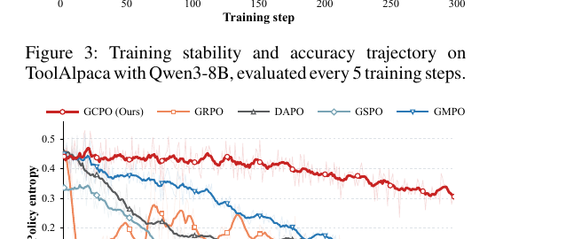
Policy entropy. A healthy RL trajectory should show entropy decreasing gradually as the policy specializes, without violent oscillation (a sign of instability) or premature collapse (a sign the policy has stopped exploring too early, which tends to hurt generalization). GRPO shows large oscillations; most other baselines show rapid, early entropy collapse; GCPO alone shows a smooth, gradual decay throughout training. This is a nice example of a secondary diagnostic (entropy dynamics weren’t the original motivation for GCPO) coming out consistent with the primary diagnostic (subspace overlap) — which is modest but real evidence that the mechanism generalizes beyond the specific metric it was designed around.

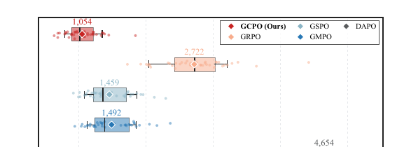
Response-length inflation. This is one of the most practically annoying RLVR failure modes: a policy discovers that padding its output with extra (often redundant or filler) tokens correlates with higher reward under a length-insensitive verifier, and the response length balloons over training without a corresponding gain in actual reasoning quality. GRPO’s median response length on MATH500 grows to 2,722 tokens; DAPO reaches 4,654 (the paper doesn’t dwell on why DAPO in particular grows the most, though DAPO’s decoupled clip-and-dynamic-sampling design is known to tolerate longer, more exploratory rollouts, which could plausibly interact with this). GCPO’s median sits at 1,054, essentially unchanged from a well-controlled baseline. The paper’s proposed mechanism is that some of the pretrained model’s principal directions plausibly encode length-related priors (e.g., stopping behavior, verbosity calibration learned during pretraining/instruction-tuning), and shielding those directions from high-variance RL gradients removes one avenue through which the policy could learn a length-based reward-hacking shortcut in the first place. This is presented as a hypothesis, not a proven mechanism, and I’d flag it as one of the paper’s more speculative claims (see Section 7) — it’s plausible but not directly tested (e.g., by looking at whether length-correlated directions actually live disproportionately in the principal subspace).

Memory efficiency. Figure 6 (peak per-GPU training memory on MATH500 with GLM4-9B) shows full-parameter GRPO, GSPO, DAPO, and GMPO all sitting around 94–96 GB, while GRPO-LoRA and GCPO both sit around 68–69 GB — essentially identical to each other. This confirms that GCPO’s extra projection operations add negligible memory overhead relative to plain LoRA, which makes sense given the earlier analysis: the added cost is a small amount of compute (two thin-matrix projections per layer per step), not additional trainable parameters or optimizer state. For practitioners already using LoRA-style adaptation for RL post-training, GCPO is close to a free upgrade in terms of resource cost.

5.5 Ablations: which design choices actually matter

Table 3 runs a systematic ablation over three independent design axes on MATH500 with GLM4-9B, and the results are genuinely informative about why GCPO works, not just that it works.

Axis	Variant	MATH500 Acc.
Projection	w/o Constraint	72.34
	Left-only	73.49
	Right-only	73.56
	Bilateral (Ours)	74.56
Subspace	Random	66.47
	Principal	62.59
	Orthogonal (Ours)	74.56
Constraints	Soft Loss Regularization	71.11
	KL Regularization	67.83
	Hard (Ours)	74.56

Projection axis — bilateral is necessary, not just nice-to-have. Constraining only the left (output) side or only the right (input) side gives a modest improvement over no constraint at all (72.34 → ~73.5), but leaves a real gap to full bilateral constraint (74.56). The mechanistic reading is straightforward: if you only seal one side, the other side is still free to align with dominant task gradients, so a unilateral constraint only partially closes the vulnerability. This directly validates the mathematical necessity of the two-sided formulation in Equations 6–7, rather than it being an arbitrary design choice.

Subspace axis — this is the most important sanity check in the paper. Deliberately constraining updates into the principal subspace (the opposite of GCPO’s actual design) causes a severe collapse to 62.59, below even the unconstrained baseline (72.34) and far below a random-subspace constraint of matched dimension (66.47). This directly confirms that it’s specifically the principal subspace — not arbitrary rank restriction, and not any arbitrary subspace — that matters. If GCPO’s gains were mostly a generic regularization effect from restricting updates to some lower-dimensional subspace, you’d expect the random-subspace variant to do reasonably well too; instead it underperforms the unconstrained baseline as well (66.47 < 72.34), and only the specifically-orthogonal-to-principal choice recovers and exceeds baseline performance. This is the single most convincing piece of evidence in the whole ablation table that the mechanism is really about this particular geometric structure of the pretrained weights, not a generic capacity-restriction effect.

Constraint-mechanism axis — hard beats soft, as predicted by the feedback-loop argument. Both a soft orthogonality loss penalty and (separately) a stronger KL regularization term underperform the hard constraint by a wide margin (71.11 and 67.83 vs. 74.56). This is exactly the failure mode predicted in Section 4.1: under RL’s iterative feedback loop, a soft penalty is one term in a sum being optimized against a reward gradient that can, and empirically does, overwhelm it. The KL-regularization variant performing worse than the soft-loss variant is a useful additional data point — it suggests that simply discouraging policy divergence in output space is a comparatively blunt instrument for preventing a specific parameter-space directional pathology; the two forms of control (output-space divergence vs. parameter-space direction) are related but not substitutable, consistent with the paper’s framing of GCPO as complementary to, not a replacement for, KL regularization.

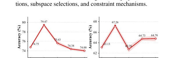
The protected rank $k$ is a real hyperparameter with a real trade-off, not a free lunch. Sweeping $k \in \{4, 8, 16, 32, 64\}$ shows accuracy peaking sharply at $k=8$ on both MATH500 and ToolAlpaca, with degradation on both sides: too small a $k$ under-protects the truly dominant directions (some principal-ish overlap is still permitted through unprotected higher-order singular directions that happen to matter), while too large a $k$ over-restricts the feasible update space, leaving too little room for genuine task adaptation. This is a legitimate design-choice discussion the paper has explicitly: the complement of an increasingly large principal subspace shrinks the space in which productive learning can happen, so $k$ is inherently a bias-variance-style trade-off between protection and capacity, not a parameter you can set-and-forget at a large “safe” value. The paper does not offer an a priori way to pick $k$ for a new model/task without running this sweep, which I’ll return to as a limitation.

5.6 Putting the ablations together: a coherent causal story

It’s worth stepping back and noting how unusually well these four independent lines of evidence (diagnostic correlation, controlled intervention, main results, ablations) reinforce rather than merely coexist with each other. The diagnostic work (Section 3) identifies when things go wrong (transient overlap spikes) and roughly where (concentrated in specific layers). The controlled intervention (Section 3.4) establishes that manipulating overlap directly changes performance, ruling out pure correlation. The main results (Section 5.2) show that removing the capacity for this overlap to occur, structurally, produces consistent gains across six independent model-task combinations with reduced variance. And the ablations (Section 5.5) show that each individual design decision inside GCPO — bilateral (not unilateral) projection, targeting specifically the principal (not random) subspace, and hard (not soft) enforcement — is doing real, separable work, rather than the aggregate improvement being attributable to any single one of these choices alone. This is a genuinely well-constructed empirical argument, and it’s part of why I’d treat this paper’s central claim with more confidence than a typical single-benchmark RL paper making a similar-sounding claim.

6. Reproducibility notes

The paper is unusually careful about reproducibility for a systems-adjacent RL paper, which is worth calling out explicitly. Fixed data splits (seed 42) are shared across all methods to avoid confounding train/test partition changes with method differences; each main configuration is independently trained across three random seeds, with mean $\pm$ std reported throughout rather than single-run numbers; the exact rollout engine (vLLM, tensor parallelism 2), precision (bf16 with FSDP), sequence-length caps (2,048 prompt / 8,192 response tokens), and per-method hyperparameters (learning rate, clipping thresholds, batch sizes) are all tabulated in the appendix. Code and datasets are released at the GitHub link in the paper header. One caveat for anyone trying to reproduce this exactly: the held-out splits for MATH500 (50 examples) and HumanEval+ (17 examples) are quite small, which is a deliberate trade-off for controlled comparison across many methods and seeds, but means per-configuration accuracy numbers should be read with the reported standard deviations in mind rather than as precise population estimates — the paper’s investment in multi-seed reporting directly compensates for this, but it’s still a smaller evaluation set than, say, a full MATH500 test split usually implies elsewhere in the literature (500 examples), since here 450 of those go to training under this paper’s held-out-split protocol.

7. Limitations the paper states, and ones it doesn’t quite

The paper’s own stated limitations (Section 5.5 in the original) are appropriately modest: it’s unclear whether the observed geometric pattern extends to non-rollout post-training paradigms like DPO, KTO, or on-policy distillation; the causal relationship between principal-subspace overlap and specific failure modes (length inflation, reward hacking) beyond the accuracy-degradation link is not fully pinned down; and the current method uses a single global $k$ per layer rather than an adaptive, layer-wise selection, which the ablation in Section 5.5 shows matters quite a bit.

Beyond what the paper states, a few things stood out to me as underexplored or understated:

• Scale. Every experiment uses 8B–9B parameter models. RL post-training instabilities, entropy collapse dynamics, and the general geometry of pretrained weight matrices are all known to shift with scale (larger models tend to have flatter singular-value spectra in some layer types, which would directly change what a “top-8” subspace even captures as a fraction of total energy). Whether the same $k=8$ sweet spot, or even the same qualitative overlap-precedes-degradation relationship, holds at 70B+ scale is genuinely an open question this paper doesn’t touch, and it’s exactly the kind of claim that’s risky to extrapolate without evidence given how much RL training dynamics are known to vary with model size.
• The length-inflation mechanism is asserted, not tested. As flagged in Section 5.4, the claim that principal directions encode “length priors” is plausible narrative glue but isn’t directly probed (e.g., via an intervention analogous to the accuracy intervention in Figure 2, but targeting length instead of correctness). Given how central this result is to the paper’s practical appeal (response-length inflation is a widely-felt pain point), a dedicated experiment here would have meaningfully strengthened the paper rather than leaving it as a hypothesis.
• The choice of $k$ isn’t given a principled selection procedure. The ablation clearly shows $k$ matters and has a real optimum, but the paper offers no cheaper alternative to a full sweep — no heuristic based on, say, the singular-value spectrum’s decay rate, the layer’s role (attention vs. MLP), or model size. For a method whose main selling point is being close to a “free” structural fix, requiring a per-model-per-task hyperparameter sweep to find $k$ is a real practical cost that the paper doesn’t fully own up to.
• Reward types are all rule-based/verifiable. All three tasks use binary or execution-based rewards rather than a learned reward model trained on human preferences. RLHF pipelines using a noisy, potentially miscalibrated learned reward model are exactly the setting where reward hacking and instability are historically worst-documented (this is literally the RLHF literature’s founding concern), and it’s an open question whether principal-subspace overlap plays the same warning-sign role when the reward signal itself is noisier and possibly exploitable in ways rule-based rewards aren’t.
• The SVD subspace is static throughout training. $\Phi_k, \Psi_k$ are computed once from $W_{\text{ref}}$ before training starts and never updated. This is a reasonable and cheap design choice, but it does mean GCPO’s notion of “dominant direction” is frozen at the pretrained checkpoint even as the effective weight $W_t$ evolves over hundreds of steps; whether the pretrained model’s principal subspace remains the most relevant one to protect deep into training (as opposed to, say, the current checkpoint’s own evolving principal subspace) is assumed rather than demonstrated.

Concrete suggestions for follow-up work: (1) run the same overlap-diagnostic pipeline at 70B+ scale to check whether the qualitative relationship (transient spikes precede degradation) and the optimal $k$ both hold, or need to be re-derived per scale; (2) design a targeted length-specific intervention (analogous to Figure 2’s accuracy intervention, but measuring response length as the outcome) to test the length-inflation mechanism directly rather than by inference; (3) develop and test a cheap heuristic for selecting $k$ per-layer from the pretrained singular-value spectrum (e.g., an elbow-detection or explained-variance threshold), removing the need for a full sweep; (4) extend the diagnostic to a setting with a learned, potentially miscalibrated reward model, to see whether principal-subspace overlap remains predictive of degradation when the reward signal itself is a plausible confound.

8. Conclusion

GCPO is a good example of a paper that earns its central design decision through careful diagnostic work rather than proposing a plausible-sounding fix and hoping it generalizes. The four-way energy decomposition, the dimension-corrected overlap statistic, and — most importantly — the controlled intervention experiment together build a genuinely convincing case that transient principal-subspace overlap is not just correlated with but at least partially causally implicated in RL post-training instability. The resulting fix is elegant precisely because it doesn’t fight the feedback loop with another soft penalty (which the ablations show fails for a specific, mechanistically-understood reason) but instead removes the problematic direction from the feasible set entirely, at essentially zero added memory cost over plain LoRA.

What I’d want to see next, beyond the scale and reward-model questions above, is whether this diagnostic lens generalizes as a general-purpose tool for understanding RL training pathologies, independent of GCPO as a specific fix — the overlap statistic itself, cheap to compute from a single SVD per layer, seems like it could be a useful monitoring signal for practitioners running any rollout-based RL recipe, not just as a design principle for a new algorithm. If a future paper shows that watching this statistic in real time and triggering a checkpoint rollback (rather than a hard architectural constraint) achieves similar stability at even lower engineering cost, that would be a natural and interesting extension of this paper’s core insight.

For practitioners deciding whether to adopt GCPO today, the practical calculus is fairly favorable: if you’re already running LoRA-style parameter-efficient RL post-training (which is now the default in many production pipelines, given full-parameter RL’s memory cost), swapping in GCPO’s projected parameterization costs you one SVD per adapted layer up front, a small constant compute overhead per step, and one extra hyperparameter ($k$) to tune — in exchange for measurably better accuracy, better cross-task retention, smoother training curves, and reduced response-length inflation, all validated across two model families and three fairly different task domains. That’s a good trade, conditional on the open questions above (particularly scale) not overturning the core finding once tested.