SwiftQK: When Normalization Becomes the Bottleneck of Tensor Parallelism

Review date: 2026-08-15 Author: Zhongzhu Zhou Paper reviewed: SwiftQK: Fast and Communication-Efficient Tensor Parallelism for Query-Key Normalization Paper authors: Gyudong Kim, Wonjun Han, Young Geun Kim (Korea University) arXiv: 2608.09160 Venue/Status: IEEE Computer Architecture Letters, preprint August 2026

1. A four-page letter about one normalization layer, and why it matters

This is a short paper — five pages including references — but it is a good specimen of a pattern that shows up constantly in real LLM-serving systems: a component that looks negligible in isolation (a normalization layer with a few floating-point operations per element) turns into the dominant latency cost once you shard the model across GPUs. SwiftQK is about exactly one such component: Query-Key Normalization (QK-Norm) under Tensor Parallelism (TP). The paper’s core empirical finding, before it proposes any fix, is startling on its own: for OLMo2 and OLMo3, which both use QK-Norm, going from 2 to 4 GPUs under TP causes the overhead of QK-Norm alone to grow from about 20% to about 30% of total latency, and 85% of that overhead is pure cross-GPU synchronization, not computation. That means for a “modern” open LLM, adding more TP-parallel GPUs increasingly buys you diminishing returns not because attention or the MLP block scales poorly, but because one particular normalization step scales badly, in a way that gets worse as you add more devices.

The fix the paper proposes, SwiftQK, is conceptually simple: instead of exchanging full Query/Key activation vectors across GPUs so each device can locally compute a normalization statistic, exchange only the scalar statistic itself, and overlap the (now much cheaper) synchronization with useful compute inside a single persistent CUDA kernel. This review will spend real time on why this problem exists in the first place — what Tensor Parallelism actually shards, why RMSNorm’s structure forces a synchronization point exactly where you don’t want one, and why prior kernel-fusion techniques for hiding communication don’t help here — before working through SwiftQK’s three-phase design, its deadlock-avoidance argument, and its numerical-precision analysis in detail.

Prerequisites: what you need to know before diving in

Tensor Parallelism (TP) and what it shards. When a language model layer is too large — or serving latency needs are too tight — to run on one GPU, Tensor Parallelism splits the computation inside a single layer across multiple GPUs, as opposed to Pipeline Parallelism (PP), which splits the model by layer and runs different layers on different devices sequentially. In the canonical Megatron-style TP layout for a Transformer block, the first linear projection in an Attention or MLP sub-layer is partitioned along its output dimension (so each GPU computes only a slice of the projected activation), while the following projection is partitioned along its input dimension so it can directly consume that local slice without any communication in between. Communication is only required once, when the final projection’s output needs to be combined across GPUs — typically via an All-Reduce. This is why TP is attractive for latency-sensitive serving on machines with fast interconnects (NVLink, NVSwitch): the two matrix multiplications inside a sub-layer talk to each other without a synchronization point in the middle, and the only required communication is one reduction at the very end of each sub-layer.

RMSNorm, and why it needs the whole vector. Root Mean Square Normalization, the normalization function used almost universally in modern open LLMs, rescales an input vector $x \in \mathbb{R}^H$ by the reciprocal of its root-mean-square magnitude:

$$\mathrm{RMSNorm}(x) = \frac{x}{\sqrt{\frac{1}{H}\sum_{j=1}^{H} x_j^2 + \epsilon}} \odot \gamma \tag{1}$$

where $H$ is the hidden dimension, $\epsilon$ is a small constant added for numerical stability (it prevents division by zero when $x$ is near-zero), and $\gamma \in \mathbb{R}^H$ is a learned per-element scaling parameter. The crucial structural fact about Eq. (1), and the entire reason this paper exists, is the denominator: $\sum_{j=1}^{H} x_j^2$ sums over every element of $x$. If $x$‘s $H$ elements are partitioned across GPUs — as they are under TP, where each GPU only holds a shard of the projected Query or Key vector — then no single GPU can compute the correct denominator from its own shard alone. Some cross-GPU communication is unavoidable; the only question is how much, and how expensive it is.

Layerwise vs. headwise QK-Norm. QK-Norm, introduced to stabilize attention logits in very large or very long-context models (originally in ViT-22B), applies RMSNorm to the projected Query and Key tensors before the scaled dot-product attention computation. It can be applied at two granularities: headwise QK-Norm computes an independent normalization factor per attention head (so the reduction in Eq. (1) only needs to span one head’s dimension, which if a head lives entirely on one GPU shard requires no communication at all), while layerwise QK-Norm computes a single normalization factor over the entire projected Q or K dimension, spanning all heads at once. The paper documents that recent open model series — OLMo2, OLMo3, and others — have converged on the layerwise formulation. This is exactly the version that breaks cleanly under TP sharding: because the whole Q/K vector for a token is split across GPUs, layerwise RMSNorm’s single global denominator forces a synchronization point squarely in the middle of what used to be a communication-free stretch of computation (projection → normalization → attention).

Why the standard fix (All-Gather) is expensive, and why simple kernel-fusion overlap tricks don’t rescue it. The default way to give every GPU what it needs to compute Eq. (1)‘s denominator is to All-Gather the full Q/K activation vector across all TP ranks before normalizing — i.e., physically move $O(H)$ elements between every pair of GPUs, reconstruct the full vector on each device, then compute the sum of squares locally. This is the “Q/K Sync (All-Gather)” step depicted by the paper’s own diagram of the modified attention block (Figure 1(b) below), and it inserts a full activation-sized communication step between the Q/K projection and the attention computation — precisely the point in the computation graph where standard (non-QK-Norm) TP has no synchronization at all. Existing kernel-fusion techniques for hiding TP communication, such as FLUX and FlashOverlap, work by overlapping a communication step with an independent, sufficiently large chunk of computation — typically the next GEMM in the pipeline — so that by the time the GEMM finishes, the communicated data has also arrived. This overlap strategy fails for QK-Norm specifically because RMSNorm’s own computation is extremely lightweight (a handful of squarings, additions, one square root, one division per element) relative to the All-Gather’s communication volume, so there simply isn’t enough independent compute available locally to hide the communication cost behind. The paper’s framing is precise: overlap-only techniques assume “communication can be hidden behind sufficient independent computation” — an assumption that holds for GEMM+All-Reduce patterns but not for RMSNorm+All-Gather.

2. Quantifying the problem before fixing it

Before presenting SwiftQK, the paper spends a full section characterizing exactly how bad the layerwise QK-Norm bottleneck is, using a controlled comparison across three model families that share almost everything except whether (and how) they use QK-Norm: OLMo (no QK-Norm), and OLMo2 / OLMo3 (both layerwise QK-Norm). Running ShareGPT-derived request traffic through vLLM’s continuous-batching engine under both Pipeline Parallelism and Tensor Parallelism on 2 and 4 A100 GPUs, the paper reports prompt-processing latency broken into three buckets: Q/K synchronization, Q/K normalization computation, and everything else.

Figure 1 (paper Fig. 1): the attention block with QK-Norm, its TP sharding pattern, and the resulting latency breakdown.

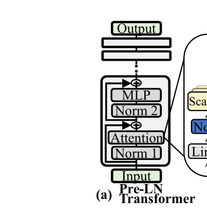
Figure 1(a) (paper Fig. 1(a)): the Pre-LN Transformer block, with QK-Norm’s two RMSNorm layers inserted directly on the projected Q and K tensors, immediately before Scaled Dot-Product Attention and after the Q/K/V linear projections.

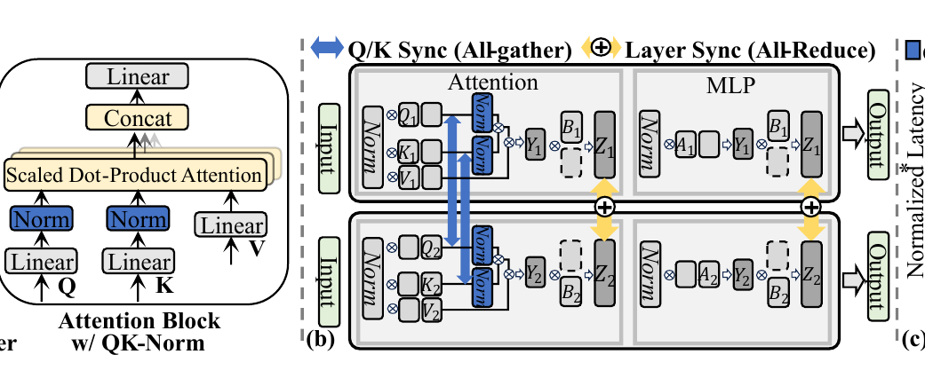
Figure 1(b) (paper Fig. 1(b)): under TP, the projected Q and K tensors are sharded across GPUs (each GPU holding $Q_1/K_1/V_1$ or $Q_2/K_2/V_2$ in the two-GPU case shown). The blue arrows denote the All-Gather Q/K synchronization step that must complete before the normalized $Q$/$K$ can feed into attention; the yellow diamond marks the separate Layer Sync (All-Reduce) that TP already requires at the end of each sub-layer, regardless of QK-Norm.

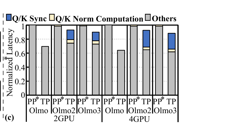
Figure 1(c) (paper Fig. 1(c)): normalized total prompt-processing latency for OLMo (no QK-Norm), OLMo2, and OLMo3 (both layerwise QK-Norm) under PP* (a PP baseline) and TP, on 2 and 4 GPUs. Latency is normalized within each model/GPU-count pair to the PP* value; the stacked bars for TP break the total into Q/K Sync (blue), Q/K Norm Computation (tan), and Others (gray).

The numbers behind Figure 1(c) are the paper’s central motivating result. For OLMo — which has no QK-Norm — going from PP to TP on 4 GPUs reduces latency by 36.2%, which is the “normal” benefit you’d expect TP to deliver by avoiding pipeline bubbles. But for OLMo2 and OLMo3, the same PP→TP switch on 4 GPUs only reduces latency by 7.5% and 12.0% respectively — a large fraction of TP’s usual advantage has been eaten by QK-Norm overhead. Digging into why: under PP, QK-Norm’s synchronization-plus-computation overhead is a rounding error, averaging only 1.4% and 1.3% of total execution time for OLMo2 and OLMo3 (because PP doesn’t shard the hidden dimension at all, so there is no cross-GPU reduction to do). Under TP, that overhead balloons to 20.0%/19.0% on 2 GPUs and grows further to 30.1%/29.7% on 4 GPUs. The growth-with-GPU-count pattern is the tell: as you shard the hidden dimension more finely across more GPUs, each GPU’s local portion of the RMSNorm computation shrinks (less work per GPU), but the synchronization cost — waiting for every peer’s partial sum to become visible — does not shrink, and in fact becomes a larger fraction of the (now smaller) total. The paper isolates the driver precisely: Q/K synchronization accounts for 73.6%/72.8% of the QK-Norm overhead on 2 GPUs, rising to 85.6%/85.5% on 4 GPUs. In other words, the computation the RMSNorm is doing is nearly irrelevant to the overhead; the overhead is almost entirely the cost of moving data (or, as we’ll see, just waiting for a handful of scalars to become visible) between GPUs.

3. SwiftQK’s design: shrink what you communicate, then hide what’s left

SwiftQK’s strategy has two independent components, and it is worth being explicit that both are necessary — the paper’s ablation-style baselines (discussed in Section 4) make clear that neither alone captures the full benefit:

1. Reduce the volume of what must cross GPUs. Instead of All-Gathering the entire $O(H)$-element Q/K activation vector so every GPU can locally recompute $\sum_j x_j^2$, have each GPU compute its own local sum of squares over just its shard, and exchange only that one scalar with its peers. This turns an $O(H)$ communication pattern into an $O(1)$ one (one float per GPU, not one vector per GPU).
2. Overlap the latency of what remains. Even after shrinking the payload to a scalar, GPUs still have to wait for every peer’s scalar to arrive before computing the global sum — this waiting time is a synchronization latency, not a volume problem, and it doesn’t disappear just because the payload got smaller. SwiftQK hides this residual latency behind other useful computation that doesn’t depend on the result of the reduction.

Algorithm 1: the fused multi-GPU persistent RMSNorm kernel

The paper packages both ideas into a single fused CUDA kernel that never launches separate communication and normalization kernels, executing per-token in three phases:

Algorithm 1 — Fused Multi-GPU Persistent RMS-Norm Kernel (reproduced from the paper, with expanded commentary)

Input: Local input shard X_local, local weights W_local,
       total hidden size H_total, number of GPUs N,
       current rank r, IPC buffers B_IPC
Output: Normalized local shard Y_local

for each token t in assigned tokens (persistent block-level stride loop):

    # ---- Phase A: Local Sum-of-Squares ----
    S_local <- BlockReduceSum( X_local[t]^2 )      # reduce over the LOCAL shard only
    if thread_id == 0:
        B_IPC[r].sumsq[t] <- S_local                # publish local scalar to IPC buffer
    __syncthreads()                                  # barrier: end of Phase A

    # ---- Phase B: Communication-Computation Overlap ----
    if warp_id == 0:
        # --- Communication path (Warp 0 only) ---
        RemoteWrite(flag) to peer GPUs               # signal "my scalar is ready"
        SpinWait(local_flag)                          # wait until all peers signal
        S_global <- sum_{k=0}^{N-1} B_IPC[k].sumsq[t]  # P2P scalar reduction
        RMS_inv  <- 1 / sqrt(S_global / H_total + eps) # global RMS factor
    else:
        # --- Computation path (remaining warps, runs CONCURRENTLY with above) ---
        for each j in assigned hidden dimensions:
            X_local[t][j] <- X_local[t][j] * W_local[j]  # weight multiply (indep. of S_global)
    __syncthreads()                                  # barrier: end of Phase B

    # ---- Phase C: Final Normalization ----
    for each j in assigned hidden dimensions:
        Y_local[t][j] <- X_local[t][j] * RMS_inv     # apply global RMS scale

Walking through why each phase exists:

Phase A — turning an $O(H)$ exchange into an $O(1)$ one. The key observation is that Eq. (1)‘s denominator only needs the scalar $\sum_j x_j^2$, not the raw vector $x$ itself. Each GPU computes this sum over only the elements it locally holds using a standard block-level parallel reduction (BlockReduceSum), then writes that single float into an inter-process-communication (IPC) buffer that peer GPUs can read directly over NVLink, without going through the host or a collective-communication library’s All-Gather primitive. This is the volume-reduction half of the design: instead of moving $H/N$ floats per GPU pair (the shard size under All-Gather), SwiftQK moves exactly 1 float per GPU pair.

Phase B — hiding the wait behind independent work. Even with only a scalar to exchange, some GPU has to be “last,” and every other GPU must wait for that scalar to become visible before it can finish computing $S_\text{global}$. This is a latency problem — an unavoidable synchronization barrier — that no amount of payload-shrinking removes. SwiftQK’s answer is to give the GPU something useful to do while it waits: it splits each CUDA block’s warps into two disjoint roles. Warp 0 is dedicated entirely to the communication path — signaling peers, spin-waiting on their signals, and performing the tiny scalar P2P reduction — while every other warp in the block performs the RMSNorm weight multiplication ($x_j \times \gamma_j$ from Eq. (1)) on the local shard, a step that is mathematically independent of $S_\text{global}$ and can therefore safely proceed before the global sum is known. This is a genuinely elegant trick: it is only possible because RMSNorm happens to factor into a normalization-scale term (which needs the global reduction) and a learned-weight multiplication term (which doesn’t), and the two can be computed in either order or in parallel.

Phase C — applying the result. Once both Phase B paths complete (enforced by the __syncthreads() barrier — all warps in the block must reach this point, meaning both the reduction and the weight multiplication are done), the final phase multiplies the already-weight-scaled local shard by the freshly-computed global RMS factor and writes the result directly to HBM. Notably, only the final normalized shard is written out — the paper is explicit that this is the only memory-hierarchy interaction beyond the IPC scalar exchange, so the kernel avoids materializing any large intermediate tensor (like the gathered full-vector Q/K that All-Gather-based QK-Norm requires) at all.

The persistent-kernel loop. The for each token t ... (persistent block-level stride loop) framing matters: rather than launching one CUDA block per token (which would require a kernel-launch-and-teardown cycle per token, and would also make the peer-synchronization logic in Phase B fragile, since blocks from different launches aren’t guaranteed to be co-resident), SwiftQK launches a bounded, fixed number of blocks once, and each resident block processes a stream of tokens in a loop, repeating Phases A–C for each one. This is what “persistent kernel” means in the GPU-programming sense, and it is also the mechanism behind the deadlock-safety argument in the next subsection.

Why deadlock-safety needs its own argument

Phase B’s SpinWait is a busy-wait: a warp spins in place, repeatedly checking a flag, until its peer’s write becomes visible. This is fine as long as the peer block that needs to write that flag is actually running concurrently — but GPUs schedule blocks onto Streaming Multiprocessors (SMs) in whatever order the hardware scheduler chooses, and if you launch more blocks than can be simultaneously resident, some blocks will be waiting in a launch queue, not yet executing at all. If Block A (already running) spin-waits on a signal from Block B (still queued, not yet scheduled), and Block B in turn needs some resource that’s only released when Block A finishes — a classic circular wait — the kernel deadlocks: every SM is occupied by a block that is stuck spinning, and no block ever finishes to free up room for the queued ones.

Why this is a real risk here, not a hypothetical. SwiftQK’s cross-GPU peer synchronization inherently requires that the corresponding block on every GPU be simultaneously resident and actively participating in the P2P handshake — if the “partner” block on GPU 2 hasn’t even been scheduled onto an SM yet, GPU 1’s Warp-0 spin-wait for GPU 2’s flag will spin forever (or until a hardware timeout), because nothing will ever come along to set that flag. This is exactly the failure mode that naive one-block-per-token kernel designs are vulnerable to at scale, and it’s the design constraint that motivates the persistent-kernel choice above rather than being a mere performance optimization.

The fix: launch only as many blocks as are guaranteed to be concurrently resident. Let $B_\text{res}$ denote the maximum number of blocks that can simultaneously reside on one SM given the kernel’s per-block resource footprint (registers, shared memory, thread count), and let $N_\text{SM}$ denote the number of SMs on the device. SwiftQK launches at most $B_\text{res} \times N_\text{SM}$ blocks — a number the CUDA occupancy calculator can determine ahead of time from the compiled kernel’s resource usage — which guarantees every launched block is resident from the moment the kernel starts, so the spin-wait in Phase B is always waiting for a block that is already running, never one that’s still queued. The persistent per-block token loop (processing multiple tokens per block, one after another, rather than launching a fresh block per token) is what lets this fixed, bounded grid still process an arbitrary number of tokens.

Design choice discussion — why not just use a library primitive with deadlock protection built in? An obvious alternative would be to rely on NCCL or a similar collective-communication library, which already has mature deadlock-avoidance logic for collective operations. The paper doesn’t use this route because collective libraries are designed around kernel-launch-boundary semantics — a collective call is typically a full kernel launch (or a sequence of them) with its own scheduling and synchronization overhead, which reintroduces exactly the kernel-launch overhead SwiftQK is trying to eliminate by fusing communication and computation into one kernel. The tradeoff SwiftQK accepts is that it must reimplement deadlock safety itself (via the bounded-grid occupancy argument above) in exchange for avoiding NCCL’s launch overhead and having fine-grained control over which warps do which work within a single kernel invocation. The boundary condition worth flagging: this occupancy-based safety argument depends on accurate knowledge of the kernel’s actual resource usage at compile/launch time; if register or shared-memory usage changes (e.g., due to a compiler version change, different data types, or a different GPU architecture with different SM resource budgets), the safe grid size must be recomputed, or the deadlock-freedom guarantee no longer holds. This is a real portability constraint that a library-based collective wouldn’t have.

4. Evaluation: does the design actually deliver, and against what?

The paper evaluates SwiftQK against four points of comparison, which is important to unpack because it’s what isolates which part of the design (volume reduction vs. latency hiding) is doing the work:

• All-Gather-based QK-Norm — the unmodified baseline: full-vector exchange, no attempt at overlap.
• Comm-Overlap — All-Gather communication overlapped with RMSNorm computation, i.e., applies the generic FLUX/FlashOverlap-style overlap idea without reducing the communication payload.
• MiniMax(eager) — scalar-statistic aggregation (same volume reduction as SwiftQK’s Phase A) but without fusing it into a single kernel or overlapping it with independent computation — communication and normalization run sequentially.
• MiniMax(fusion) — scalar aggregation further fused with RMSNorm computation into one optimized kernel (an existing vLLM implementation the paper cites), but the paper’s own results show this baseline still doesn’t achieve the same warp-level communication-computation overlap that SwiftQK’s Phase B provides.
• SwiftQK — both volume reduction and communication-computation overlap, fused into one persistent kernel.

This is a well-constructed ablation ladder: Comm-Overlap isolates “does overlap alone help without reducing volume,” MiniMax(eager) isolates “does volume reduction alone help without overlap,” MiniMax(fusion) adds fusion on top of volume reduction, and SwiftQK adds the warp-level overlap on top of that. Models tested are OLMoE (7B, Mixture-of-Experts), OLMo 2 (13B, dense), and OLMo 3 (32B, dense) — chosen specifically because they vary scale and architecture while all sharing layerwise QK-Norm, isolating the variable the paper cares about. Micro-architectural profiling runs on two NVLink-connected RTX 3090 GPUs; end-to-end serving results run on 4- and 8-GPU NVLink-connected A100 servers, with all kernels integrated into vLLM.

Figure 2 (paper Fig. 2): micro-architectural profiling, numerical-precision comparison, and end-to-end serving performance.

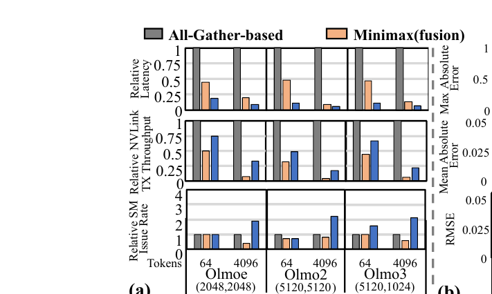
Figure 2(a) (paper Fig. 2(a)): relative latency, relative NVLink TX throughput, and relative SM issue rate, normalized to the All-Gather-based baseline, at 64 and 4096 input tokens, across OLMoE, OLMo2, and OLMo3. SwiftQK shows the lowest relative latency in every configuration while simultaneously showing the highest SM issue rate — evidence that Warp 0’s communication path and the other warps’ computation path really are running concurrently rather than one blocking the other.

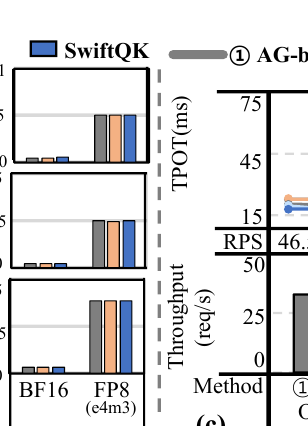
Figure 2(b) (paper Fig. 2(b)): mean-absolute-error and RMSE of All-Gather-based, MiniMax(fusion), and SwiftQK against a gold-standard full-precision (FP64) RMSNorm reference, for both BF16 and FP8 (e4m3) activations. SwiftQK’s error is comparable to the other methods’, not larger — i.e., the accumulation-order changes introduced by scalar partial-sum aggregation don’t introduce extra numerical error beyond what the underlying low-precision format already contributes.

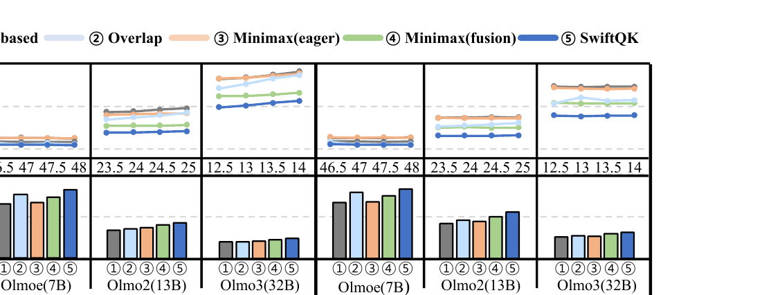
Figure 2(c) (paper Fig. 2(c)): time-per-output-token (TPOT, lower is better) and saturated request throughput (higher is better) for the five compared methods, across OLMoE/OLMo2/OLMo3 on 4 and 8 GPUs, sweeping request rate (RPS) below saturation. SwiftQK (⑤, dark blue) sits consistently below the other four curves in every TPOT panel and above them in every throughput bar.

Reading the numbers. In the micro-architectural profiling (Figure 2(a)), SwiftQK reduces QK-Norm latency by 81.4–93.9% relative to All-Gather-based QK-Norm, and by a further 29.4–77.0% relative to MiniMax(fusion) — the latter comparison is the important one, because it isolates the marginal benefit of SwiftQK’s warp-level overlap on top of volume reduction and fusion that MiniMax(fusion) already has. At 4096 tokens, SwiftQK achieves 2.8–4.6× higher SM issue rate than MiniMax(fusion), directly evidencing that SwiftQK’s Warp-0/other-warps split really is keeping compute units busier during the communication wait, rather than the reported latency win coming from some unrelated kernel-efficiency difference.

On numerical precision (Figure 2(b)), the paper’s concern is legitimate and worth taking seriously: reordering how a sum is accumulated (per-GPU-shard local sums combined via P2P scalar reduction, versus one giant reduction over the reconstructed full vector) can in principle change floating-point rounding behavior, since floating-point addition is not associative. SwiftQK’s mitigation is to accumulate both the local squared-sum and the cross-GPU scalar reduction in FP32, even when the underlying activations are stored in BF16 or FP8-E4M3. Measured against an FP64 gold reference, SwiftQK’s maximum-absolute, mean-absolute, and RMS errors (5.0e-2, 2.1e-3, 3.4e-3 for BF16; 5.0e-1, 2.5e-2, 3.9e-2 for FP8) track closely with the other methods’ — i.e., SwiftQK’s design doesn’t introduce meaningfully more numerical drift than what the BF16/FP8 formats themselves already impose. This is a genuinely important check for a systems paper making a change to the accumulation pattern of a numerically-sensitive normalization operation, and the paper deserves credit for including it rather than only reporting speed numbers.

On end-to-end serving (Figure 2(c)), SwiftQK reduces average TPOT by 29.5% and increases saturated throughput by 25.4% relative to the All-Gather baseline; against the two intermediate baselines it reduces TPOT by 17.9% (vs. Comm-Overlap) and 28.5% (vs. MiniMax(eager)), with throughput gains of 14.6% and 20.1% respectively. Most tellingly for the paper’s central claim, even against MiniMax(fusion) — already scalar-aggregating and already fused — SwiftQK still reduces TPOT by 14.3% and lifts throughput by 8.8%. The paper’s own framing of this last comparison is the right one: it demonstrates that SwiftQK’s end-to-end benefit “is not only from scalar-statistic aggregation, but also from combining reduced communication volume with fused persistent execution and in-kernel communication-computation overlap” — i.e., both halves of the design (Section 3’s two numbered strategies) are independently contributing, not just one of them doing all the work while the other is along for the ride.

4b. A worked numerical walkthrough of Algorithm 1

It helps to see Algorithm 1 run on concrete numbers rather than only symbols, so let’s trace through one token on a toy 2-GPU TP setup with a total hidden dimension $H_\text{total} = 8$, split evenly so each GPU holds $H_\text{local} = 4$ elements of the projected Query vector for one token, with $\epsilon = 10^{-6}$ and $\gamma_j = 1$ for all $j$ (to keep the arithmetic legible).

Suppose the true (un-sharded) projected Q vector for this token is

$$x = [\,1.0,\ 2.0,\ -1.0,\ 0.5,\ 3.0,\ -2.0,\ 1.5,\ 0.5\,] \tag{2}$$

with GPU 0 holding the first 4 elements $x^{(0)} = [1.0, 2.0, -1.0, 0.5]$ and GPU 1 holding the last 4, $x^{(1)} = [3.0, -2.0, 1.5, 0.5]$.

Phase A on each GPU. Each GPU computes its own local sum of squares:

$$S_\text{local}^{(0)} = 1.0^2 + 2.0^2 + (-1.0)^2 + 0.5^2 = 1.0 + 4.0 + 1.0 + 0.25 = 6.25 \tag{3}$$ $$S_\text{local}^{(1)} = 3.0^2 + (-2.0)^2 + 1.5^2 + 0.5^2 = 9.0 + 4.0 + 2.25 + 0.25 = 15.5 \tag{4}$$

Each GPU writes exactly one scalar ($6.25$ or $15.5$) into its IPC buffer slot for this token. Contrast this with All-Gather-based QK-Norm, which would instead move the entire 4-element shard from each GPU to its peer — 4 floats each way, not 1.

Phase B: the P2P reduction, running concurrently with weight multiplication. Warp 0 on each GPU reads both IPC scalars once both are visible:

$$S_\text{global} = S_\text{local}^{(0)} + S_\text{local}^{(1)} = 6.25 + 15.5 = 21.75 \tag{5}$$ $$\mathrm{RMS}^{-1} = \frac{1}{\sqrt{S_\text{global}/H_\text{total} + \epsilon}} = \frac{1}{\sqrt{21.75/8 + 10^{-6}}} = \frac{1}{\sqrt{2.71875 + 10^{-6}}} \approx \frac{1}{1.6489} \approx 0.6065 \tag{6}$$

While Warp 0 is computing Eqs. (5)-(6) — which requires waiting for both scalars to be visible, the one genuine synchronization latency in the whole kernel — the other warps on each GPU are simultaneously computing $x_j^{(r)} \times \gamma_j$ for their local shard. Since $\gamma_j = 1$ in this toy example, this step is a no-op numerically, but in the general case (learned $\gamma \ne 1$) this is real, independent work happening in parallel with the wait in Eqs. (5)-(6).

Phase C: applying the global factor. Each GPU multiplies its (already weight-scaled) local shard by the shared $\mathrm{RMS}^{-1} \approx 0.6065$:

$$y^{(0)} = 0.6065 \times [1.0, 2.0, -1.0, 0.5] \approx [0.607, 1.213, -0.607, 0.303] \tag{7}$$ $$y^{(1)} = 0.6065 \times [3.0, -2.0, 1.5, 0.5] \approx [1.820, -1.213, 0.910, 0.303] \tag{8}$$

Sanity check against the un-sharded computation. Computing RMSNorm directly on the full 8-element vector $x$ from Eq. (2) gives $\sum x_j^2 = 6.25 + 15.5 = 21.75$ — identical to $S_\text{global}$ in Eq. (5), confirming that the sharded, two-phase computation is exactly mathematically equivalent to the un-sharded one (up to floating-point rounding order), not an approximation. This is the point the paper is making when it says SwiftQK preserves “the same global normalization semantics”: Eqs. (3)-(8) reduce an $O(H)=8$-element cross-GPU exchange to a 2-scalar exchange (1 scalar per GPU pair direction) while computing bit-for-bit (modulo FP32 accumulation order) the same output as the reference All-Gather path.

Where the communication savings scale from. In this toy example the saving is only 4 floats reduced to 1 (a 4× reduction), because $H_\text{local}=4$ is small. In a real deployment, a 13B-parameter model’s per-GPU Q/K shard under 4-way TP might hold on the order of $H_\text{local} \approx 1024$-$2048$ elements (depending on head count and TP degree) — so the same Phase A trick reduces an exchange of over a thousand floats per GPU pair to a single scalar, an over-1000× reduction in raw payload, which is consistent with the paper’s reported 81-94% latency reduction being dominated by volume rather than by the overlap trick alone (the overlap trick contributes the additional 29-77% improvement over MiniMax(fusion), which already has the volume reduction).

4c. How SwiftQK’s approach compares to other communication-reduction strategies for TP

It is useful to place SwiftQK’s approach on a spectrum with other communication-reduction techniques the broader TP/serving literature has explored, to see precisely what is and is not novel about its combination of ideas.

Technique	Reduces communication volume?	Overlaps residual latency?	Fused into one kernel?	Applicable to QK-Norm’s global-reduction pattern?
Standard All-Gather TP	No (full vector)	No	No (separate comm + norm kernels)	Yes (baseline)
FLUX / FlashOverlap (GEMM+comm overlap)	No	Yes, but only when compute-to-communication ratio is large	Partially (comm/GEMM fusion)	No — RMSNorm’s compute is too light to hide All-Gather behind
MiniMax(eager) scalar aggregation	Yes ($O(H)\to O(1)$)	No (sequential comm then norm)	No	Yes
MiniMax(fusion)	Yes	No warp-level overlap	Yes (comm + norm fused)	Yes
SwiftQK	Yes	Yes (warp-level, in-kernel)	Yes (single persistent kernel)	Yes
Headwise QK-Norm (architectural avoidance)	N/A — avoids the reduction entirely by keeping each head’s normalization local to one GPU shard	N/A	N/A	Sidesteps the problem rather than solving it

The table makes explicit what Section 4’s ablation ladder already showed empirically: SwiftQK isn’t introducing a fundamentally new idea in isolation — scalar-statistic aggregation already existed (MiniMax-eager), and comm/compute overlap already existed (FLUX/FlashOverlap) — its contribution is recognizing that RMSNorm’s specific structure (additively-decomposable global statistic, plus an independent weight-multiplication term) lets both existing ideas be combined into a single fused, deadlock-safe, persistent kernel in a way that neither idea achieves alone, and that this specific combination is what’s needed because RMSNorm is too lightweight for generic GEMM-style overlap and too latency-sensitive for scalar aggregation without overlap to be sufficient on its own.

5. Design-choice discussion: why these choices, what the alternatives were, and where they might break

Why scalar aggregation instead of a smarter partial All-Gather (e.g., hierarchical or tree-based reduction)? A tree-based or hierarchical All-Gather could, in principle, reduce the effective communication cost of exchanging the full vector by routing it more efficiently across the NVLink topology, without reducing the raw data volume. SwiftQK’s approach is strictly better in the volume dimension — it reduces what needs to move from $O(H)$ elements to $O(1)$ regardless of topology — but the tradeoff is that this only works because RMSNorm’s global statistic reduces to a single sum of squares; it would not generalize as cleanly to a normalization scheme whose global statistic needed more than one scalar (for instance, a scheme requiring both a mean and a variance, or requiring cross-token statistics rather than purely per-token ones). The boundary condition here is architectural: SwiftQK’s trick is specific to reduction-based normalization statistics that decompose additively across shards, and would need rethinking for normalization variants whose statistics don’t decompose this way.

Why split work by warp rather than by, say, time-multiplexing the same warps between communication and computation? Assigning Warp 0 exclusively to the communication path and the rest to computation is a static partition decided at kernel-design time, not at runtime. The obvious alternative — having all warps interleave between checking the communication flag and doing element-wise work — would avoid “wasting” one warp’s compute capacity on what is mostly spin-waiting, but it would complicate the correctness argument considerably (you’d need careful reasoning about exactly when each warp checks the flag versus does compute, rather than a clean two-path split), and it risks introducing exactly the kind of subtle scheduling bug that a persistent, deadlock-sensitive kernel can least afford. The paper’s static partition is the more conservative, easier-to-verify choice, at the cost of some SM issue-rate headroom on Warp 0 specifically (though the reported 2.8–4.6× SM issue-rate advantage over MiniMax(fusion) suggests this cost is not large in practice). The boundary condition: as $H$ (head dimension × number of heads under one GPU’s shard) grows very large relative to the number of warps in a block, giving up one full warp’s worth of compute to communication becomes proportionally cheaper; for very small hidden-dimension shards (e.g., aggressive TP degrees on small models), dedicating an entire warp to what is fundamentally a few-scalar exchange could become a comparatively larger fixed cost, though the paper does not report a regime where this cost becomes dominant.

Why FP32 accumulation specifically, rather than staying in the native (BF16/FP8) precision throughout? Accumulating a sum of squares in BF16 or FP8 directly would compound rounding error especially badly, since squaring already narrows the effective dynamic range being summed and low-precision formats have few mantissa bits to absorb accumulated rounding. FP32 accumulation is a standard mitigation (also used in, e.g., mixed-precision training accumulators) that costs essentially nothing extra in this setting because the reduction itself operates on a single scalar per GPU, not a full tensor, so promoting that one value to FP32 for the accumulation step is nearly free. The alternative of accumulating in native low precision would have been strictly worse and is correctly avoided; the paper’s contribution here is not novel numerically, but it is a necessary and correctly-applied piece of engineering hygiene that a less careful implementation could easily have skipped.

Why is the paper’s baseline comparison set limited to Megatron-style intra-layer TP, without discussing sequence-parallelism or expert-parallelism interactions? This is more a scope observation than a criticism of a specific choice, but it’s worth naming as a design boundary: SwiftQK is evaluated purely in the context of standard tensor-parallel attention/MLP sharding. Many production serving stacks combine TP with sequence parallelism (which additionally shards the sequence dimension for parts of the forward pass) or, for MoE models like OLMoE, expert parallelism (which shards along the expert dimension rather than the hidden dimension). The paper does test OLMoE, but only under the same TP-sharding assumptions as the dense models; it does not discuss how SwiftQK’s per-GPU-shard reduction pattern interacts with a scenario where the Q/K hidden dimension is sharded differently than the expert-routing dimension, which is a real deployment configuration for large MoE models at scale.

5b. Formalizing the deadlock-freedom argument

Section 3’s deadlock-safety discussion is worth making fully rigorous, since it’s the load-bearing correctness property of the whole design (a fast kernel that occasionally hangs is worse than a slow one that never does).

The hazard, stated as a graph problem. Model each CUDA block’s execution as a node in a wait-for graph: block $u$ has an edge to block $v$ if $u$ is spin-waiting on a signal that only $v$ can produce. A kernel deadlocks if and only if this wait-for graph contains a cycle and the blocks on that cycle are never all simultaneously scheduled. Concretely, in SwiftQK’s Phase B, the peer-blocks handling the same token index $t$ across all $N$ GPUs form a strongly-connected component in the wait-for graph — each GPU’s Warp 0 waits on every other GPU’s IPC write for that token before it can compute $S_\text{global}$. This is unavoidable given the algorithm (the global sum genuinely needs every shard’s contribution) — so the only lever available to prevent deadlock is guaranteeing all members of this strongly-connected component are concurrently resident and executing, never queued.

Why bounding the grid size is sufficient (not just necessary). The GPU hardware scheduler guarantees that once a block is dispatched to an SM, it runs to completion without preemption by another block (ignoring rare context-switch scenarios not relevant here), and that it will make forward progress as long as it isn’t blocked on an external event. If SwiftQK launches exactly $B_\text{res} \times N_\text{SM}$ blocks — the maximum number the occupancy calculator determines can be concurrently resident given the kernel’s compiled register/shared-memory footprint — then by construction every launched block is dispatched to some SM at kernel-launch time (none are left in a launch queue waiting for a slot to free up). Since the corresponding blocks on every peer GPU are launched with the identical bound, and all GPUs execute the identical launch simultaneously (this is implicit in how the paper structures a single logical kernel invocation spanning all TP ranks), every member of a token’s cross-GPU strongly-connected component is guaranteed to be resident from time zero — closing off the only path to deadlock. This is why the bound needs to be at most $B_\text{res} \times N_\text{SM}$ (any fewer is also safe, just less parallel; any more reintroduces a launch queue and the hazard).

A subtlety the paper’s presentation glosses over: the persistent stride loop’s within-block ordering. Because each resident block processes multiple tokens in sequence (the persistent stride loop), and different blocks may progress through their assigned tokens at different rates (due to, e.g., memory-access latency variance), it’s worth checking that a block processing token $t+1$ never needs to wait on a peer block that is still stuck processing token $t$‘s Phase B in a way that could stall the whole kernel rather than just that one block’s throughput. Because each token’s Phase B synchronization only involves the specific peer blocks assigned to that same token index (not a global barrier across all resident blocks), a block that finishes token $t$ early can proceed to Phase A of token $t+1$ without waiting for unrelated blocks handling different tokens — the design is correctly scoped so that cross-block dependency exists only within a token’s processing, not across tokens. This is implicit in the algorithm’s structure but worth stating explicitly, since a naive persistent-kernel implementation that accidentally introduced a global cross-token barrier would reintroduce unnecessary serialization even without technically deadlocking.

5c. Practical deployment considerations beyond the paper’s own evaluation

A few operational questions a systems engineer evaluating SwiftQK for production deployment would reasonably ask, going beyond what Section 4’s benchmark suite covers:

Interaction with dynamic batching and variable sequence lengths. vLLM-style continuous batching means the set of active tokens being processed changes every iteration, and different requests in a batch may be at different stages of prefill versus decode. SwiftQK’s persistent kernel needs to correctly handle a token-count-per-iteration that varies from one scheduler step to the next, since the fixed grid of $B_\text{res} \times N_\text{SM}$ blocks must gracefully handle both a large prefill batch (many tokens, each block processing several in its stride loop) and a small decode-only batch (potentially fewer tokens than resident blocks, in which case some blocks simply have no work in a given iteration). The paper’s integration into vLLM implies this is handled, but the letter format doesn’t have room to describe the scheduling-integration logic in detail.

Failure and straggler handling. The SpinWait primitive in Phase B has no explicit timeout or failure-detection mechanism described in the paper. In a production multi-GPU serving fleet, a peer GPU can become slow (thermal throttling, an unrelated process momentarily occupying SMs, ECC-induced compute retries) or, in the worst case, fail entirely (driver crash, Xid error). A spin-wait with no timeout in the failure case would hang the entire pipeline stage indefinitely rather than degrading gracefully — this is a genuine operational risk for any system built on this primitive that the letter’s scope does not address, and would need to be handled by a surrounding supervisory layer (e.g., a watchdog that can detect and restart a stalled kernel) that isn’t described.

Portability across GPU architectures. The reported results are specific to NVLink-connected RTX 3090 (consumer-class, Ampere) and A100 (datacenter-class, also Ampere) GPUs. Newer architectures (Hopper, Blackwell) have different SM resource budgets, different NVLink generations with different latency/bandwidth characteristics, and in some cases hardware-level primitives for exactly this kind of small-message peer synchronization (e.g., NVLink Switch multicast or newer cluster-communication primitives) that could either make SwiftQK’s hand-rolled IPC-buffer approach less necessary or could be leveraged to make it even faster — the paper doesn’t discuss whether the $B_\text{res} \times N_\text{SM}$ occupancy calculation and the persistent-kernel structure would need re-tuning (or would even remain optimal) on newer hardware generations.

6. Limitations, as the paper itself acknowledges (and a few it doesn’t)

The paper is admirably candid about the narrowness of its own scope. It’s explicit that QK-Norm placement and definition within Transformer blocks is still an evolving design space (citing ongoing exploration of alternative normalization strategies), and it explicitly flags that its contribution generalizes only to normalization schemes that “span TP-partitioned activations and require cross-GPU synchronization” — i.e., the trick doesn’t automatically transfer to every normalization variant a future model might adopt. It also limits its evaluation to a specific hardware substrate (NVLink-connected RTX 3090 and A100 GPUs), and to three specific OLMo-series models, without testing on other model families that use QK-Norm (e.g., Gemma or Qwen variants that have adopted similar normalization), leaving open whether the observed overhead percentages and speedups generalize to architectures with different head-dimension-to-total-hidden-dimension ratios.

7. Critical analysis

Weaknesses and flaws specific to this paper. First, the evaluation is entirely confined to NVLink-class interconnects, where peer-to-peer bandwidth and latency are both favorable; the paper gives no indication of how the persistent spin-wait pattern in Phase B behaves on PCIe-only multi-GPU setups (common in cheaper or older serving deployments) or on multi-node configurations where inter-GPU communication must cross a network fabric rather than NVLink — a spin-wait strategy that’s cheap on NVLink (microsecond-scale round trips) could become a genuinely wasteful busy-wait on higher-latency links, and the paper offers no fallback or discussion for this case. Second, the deadlock-safety argument, while logically sound, rests entirely on the assumption that the occupancy calculation ($B_\text{res} \times N_\text{SM}$) is computed correctly and stays valid at runtime; the paper doesn’t discuss what happens if the kernel is launched alongside other concurrent kernels on the same GPU (a common scenario in a real multi-tenant serving system, where QK-Norm computation for one model might share SMs with unrelated work from another request or model), which could change the number of blocks that are actually concurrently resident versus what the static occupancy calculation predicted, silently reintroducing the deadlock risk the paper claims to have eliminated. Third, the ablation set (All-Gather, Comm-Overlap, MiniMax(eager), MiniMax(fusion), SwiftQK) is a reasonable ladder, but the paper doesn’t report variance or confidence intervals across repeated runs for any of its latency or throughput numbers — for a paper whose central claims rest on percentage differences in the 10–30% range measured on shared hardware (GPUs can have run-to-run variance from thermal throttling, driver-level scheduling jitter, etc.), the absence of any error bars or repeated-trial statistics is a real gap in rigor.

Limitations the authors understate or omit. The paper frames headwise QK-Norm as basically communication-free (“if a head lives entirely on one GPU shard requires no communication at all” is this reviewer’s inference from the paper’s own framing, not an explicit claim, but the paper does contrast layerwise against headwise as the reason layerwise is the harder case) — but it never actually benchmarks a model using headwise QK-Norm to confirm this baseline assumption empirically; the entire motivating comparison in Section 2/Figure 1 is built around models using layerwise QK-Norm exclusively, so the reader has to take the “headwise is essentially free” framing on faith rather than seeing it validated against actual headwise-QK-Norm models like ViT-22B or any LLM that has adopted the headwise variant. Separately, the paper’s persistent-kernel design necessarily holds a fixed, bounded set of CUDA blocks resident on every GPU for the entire duration of every forward pass through every layer that uses QK-Norm — this is a real occupancy tax (the GPU can’t use those SM slots for anything else while the persistent kernel is resident) that the paper does not quantify; a persistent kernel that must remain resident to service RMSNorm calls in a model with dozens of QK-Norm layers could meaningfully constrain how much SM capacity is available for the surrounding GEMM-heavy attention and MLP computation, and this cost is not reported anywhere in the evaluation.

Concrete, specific improvement suggestions. (1) Report tail-latency percentiles (p99 TPOT), not just averages — a communication-bound operation with a busy-wait component is exactly the kind of code path where tail behavior under contention (e.g., when one peer GPU is momentarily slower due to thermal throttling or an unrelated kernel occupying its SMs) can diverge sharply from the mean, and the paper’s current TPOT numbers give no visibility into this. (2) Add an explicit fallback mode, or at minimum a discussion, for non-NVLink interconnects (PCIe, multi-node RDMA), since the spin-wait design’s cost-benefit tradeoff depends heavily on peer-to-peer latency, and many real deployments (especially cost-sensitive inference-serving fleets) do not have NVLink available on every GPU pair. (3) Quantify the persistent-kernel occupancy tax directly — report, for a representative model, what fraction of total SM-seconds across a full forward pass are consumed by SwiftQK’s resident blocks versus available to the surrounding GEMM computation, so a systems engineer evaluating the tradeoff can reason about it quantitatively rather than qualitatively. (4) Extend the evaluation to at least one model using headwise QK-Norm, to empirically validate (rather than assume) that the headwise variant is indeed communication-free under TP, which would strengthen the paper’s framing of layerwise QK-Norm as the uniquely problematic case.

8. Reproducibility notes

The paper cites its baselines with enough specificity to be independently reproducible in spirit: All-Gather-based QK-Norm is described as the standard TP implementation; MiniMax(fusion) is explicitly cited as an existing, publicly available vLLM kernel (rms_norm_tp.py, referenced by commit hash 99a8561 in the vLLM GitHub repository), which gives a concrete, checkable artifact for anyone wanting to reproduce the comparison baseline. The evaluated models (OLMoE-7B, OLMo2-13B, OLMo3-32B) are all openly released model checkpoints from the Allen Institute for AI’s OLMo series, and the request workload (ShareGPT) is a standard, publicly available dataset. What is not fully specified in the letter (understandably, given the four-page IEEE CAL format constraint) is the exact CUDA/driver/vLLM version pinning used for the reported numbers, the specific occupancy-calculator output ($B_\text{res}$ values) used per GPU architecture, or the exact micro-benchmark harness used to produce Figure 2(a)‘s token-count sweep — a reader wanting to exactly reproduce the reported percentage improvements would need to either contact the authors for these details or reconstruct them from the vLLM integration referenced in the paper.

8b. A glossary of the paper’s abbreviated terms, for quick reference

• TP (Tensor Parallelism): sharding computation within one layer across GPUs, as opposed to PP.
• PP (Pipeline Parallelism): sharding a model by layer across GPUs, running different layers on different devices in sequence.
• QK-Norm: applying RMSNorm to the projected Query and/or Key tensors before attention, to stabilize attention logits.
• Layerwise QK-Norm: one normalization factor spanning the entire projected Q/K dimension (all heads together).
• Headwise QK-Norm: an independent normalization factor per attention head.
• All-Gather: a collective communication primitive that reconstructs a full tensor on every participating device by exchanging each device’s local shard.
• IPC buffer: a memory region accessible directly by peer GPUs over NVLink (Inter-Process Communication), bypassing host-mediated data transfer.
• TPOT (Time Per Output Token): the average latency between consecutive generated tokens during decode, a standard LLM-serving latency metric.
• RPS (Requests Per Second): the offered request rate used to sweep serving load below the saturation point.
• $B_\text{res}$: the maximum number of CUDA blocks with SwiftQK’s specific register/shared-memory footprint that can be concurrently resident on one SM.
• $N_\text{SM}$: the number of Streaming Multiprocessors on the target GPU.

9. What this means if you’re building or operating a TP-serving stack

If you’re operating a serving system on QK-Norm-using models under Tensor Parallelism today, the paper’s Section 2 characterization alone is actionable independent of whether you adopt SwiftQK specifically: it’s worth profiling how much of your own TP latency, at your own TP degree, is attributable to QK-Norm synchronization versus everything else, especially if you’ve observed diminishing returns from adding more TP-parallel GPUs. If that overhead is significant, SwiftQK’s core idea — reduce cross-GPU exchange to the minimal sufficient statistic, and overlap the residual synchronization latency with independent computation inside one fused kernel — is a pattern worth applying even outside the specific RMSNorm case: any per-token, per-shard reduction-based normalization or statistic computation under TP is a candidate for the same scalar-aggregation-plus-overlap treatment, provided its global statistic decomposes additively across shards the way a sum of squares does.