Chasing a Moving Target: Calibration and Rank-Allocation Drift in Training-Free Low-Rank LLM Compression

Review date: 2026-08-14 Author: Zhongzhu Zhou Paper reviewed: Understanding Calibration and Truncation Error Propagation in Training-Free Low-Rank Compression for LLMs Paper authors: Mohanad Odema, Gabrielle De Micheli, Dayin Gou, Nilesh Malpeddi, Prathamesh Vaste, Jacob Song (LG Electronics, North America) arXiv: 2608.08506 Venue/Status: Published as a conference paper at COLM 2026

Prerequisites

Before diving into the paper’s contribution, it helps to be comfortable with a handful of ideas. If you already know these, feel free to skip to “Two Sources of Drift” below.

Why compress LLMs at all

Modern LLMs carry billions of parameters. Serving them costs GPU memory and latency, and deploying them on edge devices (phones, laptops, in-car assistants) is often outright infeasible without shrinking the model. Three families of compression techniques dominate the literature:

• Pruning — remove weights or entire structural units (neurons, attention heads, layers) that contribute little to the output.
• Quantization — represent weights (and sometimes activations) with fewer bits, e.g. INT8/INT4 instead of BF16.
• Low-rank decomposition — replace a weight matrix with a product of two (or more) much smaller matrices, exploiting the fact that many trained weight matrices have most of their “useful” information concentrated in a small number of singular directions.

This paper is about the third family. It targets training-free low-rank compression, meaning: no gradient-based fine-tuning after compression (no recovery fine-tuning, “RFT”), no expensive second-order (Fisher information) estimates — just a forward pass or two over a small calibration set, then closed-form linear algebra.

Singular Value Decomposition (SVD) refresher

Any matrix $W \in \mathbb{R}^{m \times n}$ can be exactly factored as

$$W = U \Sigma V^T$$

where $U \in \mathbb{R}^{m \times m}$ and $V \in \mathbb{R}^{n \times n}$ are orthogonal, and $\Sigma$ is diagonal with non-negative singular values sorted in decreasing order. If we keep only the top $r$ singular values/vectors, we get a rank-$r$ approximation

$$\hat{W} = U_r \Sigma_r V_r^T,$$

which is provably the best rank-$r$ approximation to $W$ under the Frobenius norm (Eckart–Young theorem). The intuition: singular values measure “how much” each orthogonal direction contributes to the matrix’s action, so keeping only the largest ones discards the least useful directions. The number of parameters drops from $mn$ to $r(m+n)$, which is a big win when $r \ll \min(m,n)$.

From plain SVD to activation-aware SVD

Plain SVD on the raw weight matrix ignores how the weight is actually used. If most inputs $x$ live in a narrow subspace of $\mathbb{R}^n$, then a weight direction that is rarely excited by real inputs doesn’t need to be preserved as carefully as a weight direction that is heavily used, even if the two directions have similar singular values in isolation. Activation-aware decomposition methods incorporate a small calibration dataset (a few hundred examples, e.g. from WikiText-2) to estimate the input covariance statistics, and then decompose the weight in a way that minimizes the reconstruction error of the output activations rather than the raw weight entries:

$$O = \min \left( \| WX - \hat{W} X \|^2 \right)$$

Here $X$ is the calibration activation matrix (rows/columns are calibration tokens passed through the model up to that layer). This is the per-weight decomposition objective used by earlier work like SVD-LLM.

Joint (module-level) decomposition

A newer generation of methods (MoDeGPT, UniQL) observed that compressing each weight matrix independently ignores the fact that neighboring matrices within a transformer block (e.g. the up/gate/down projections of an MLP, or the Q/K/V/O projections of attention) interact nonlinearly. So instead of a per-weight objective, they minimize a module-level reconstruction loss:

$$O = \min \Big( f(\|X; W_1, \cdots, W_k\|^2) - f(\|X; \hat W_1, \cdots, \hat W_k\|)\Big)^2$$

where $f$ is the module’s actual forward function (e.g. the full MLP forward pass, non-linearity included) and $W_1, \ldots, W_k$ are all the weight matrices inside that module. This “joint decomposition” consistently beats per-weight decomposition in accuracy, because it accounts for how errors in one matrix interact with the others through the non-linearity.

Non-uniform rank allocation and the Block Influence (BI) score

Not all transformer layers are equally important. Early low-rank methods used a single, uniform compression ratio for every layer. But some layers barely transform their input (redundant, easy to compress hard) while others induce large changes (important, should be preserved). A widely used proxy for “how much a layer transforms its input” is the Block Influence (BI) score (from ShortGPT):

$$\mathrm{BI}_i = 1 - \mathrm{CosSim}(X_i, X_{i+1})$$

where $X_i, X_{i+1}$ are the input and output activations of layer $i$, and $\mathrm{CosSim}$ is cosine similarity. A layer that barely changes its input direction (high cosine similarity, low BI) is considered less important and can absorb a more aggressive compression ratio; a layer that transforms its input dramatically (low cosine similarity, high BI) is considered important and should be preserved closer to full rank. These per-layer BI scores are converted into per-layer rank ratios via a temperature-scaled softmax that also respects a global compression budget — we will look at the exact formula shortly.

With those building blocks in place, we’re ready for the paper’s actual contribution.

Two Sources of Drift That Nobody Was Correcting

The central observation of this paper is refreshingly simple to state, and yet nobody had rigorously quantified it before: existing training-free low-rank pipelines treat the original, uncompressed model as a fixed reference throughout the entire compression process — but that reference silently becomes stale as compression proceeds. There are two distinct ways this staleness shows up.

Drift #1: Calibration Error Residuals

Standard practice: pass ~128 calibration samples through the original, uncompressed model once, capture the activation statistics at every layer, and use those (frozen) statistics to decide how to compress every layer. The implicit assumption is that these captured activations are a faithful proxy for what the final compressed model will actually see at inference time.

But that assumption breaks down as soon as you start compressing. Once layer 1 is compressed, its output activations are no longer identical to the original model’s layer-1 output — there is some reconstruction error. When that (slightly wrong) activation gets fed into layer 2’s calibration statistics estimation — except layer 2’s statistics were pre-computed using the original (uncompressed) layer 1’s output, not the actual compressed layer 1’s output — the mismatch compounds.

The paper measures this directly with a normalized mean squared error (NMSE) metric:

$$\mathrm{NMSE} = \frac{\sum (x - \hat x)^2}{\sum x^2}$$

comparing the original model’s activations $x$ against the compressed model’s activations $\hat x$ at each layer.

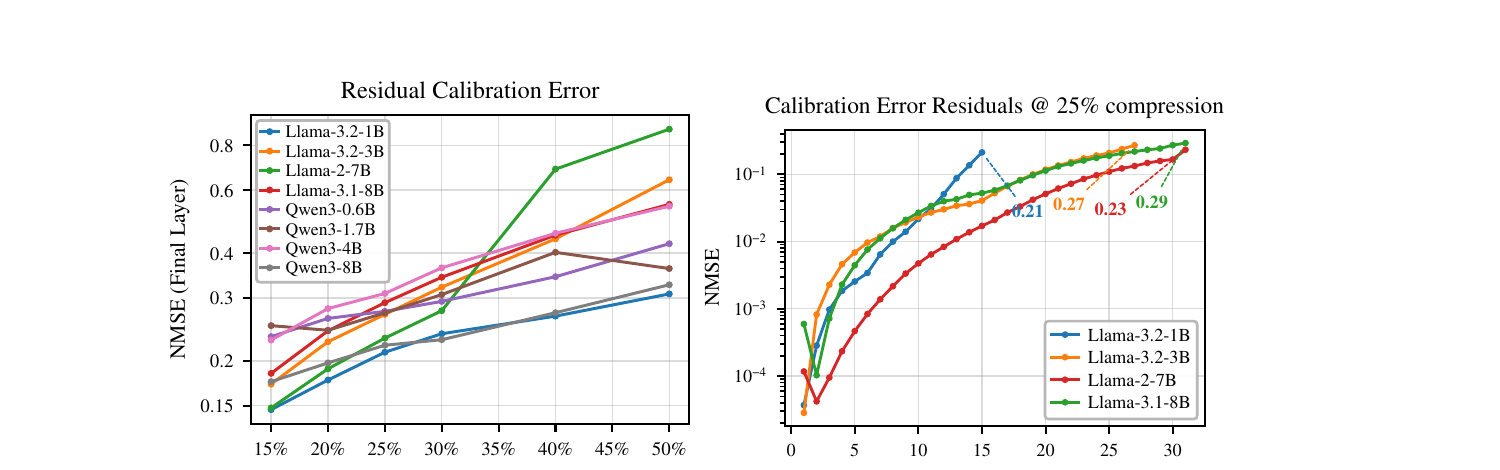
The left panel of Figure 1 sweeps compression rate (15%–50%) and plots the final-layer NMSE for 8 different models. Every single model shows the same qualitative trend: NMSE climbs steadily as compression becomes more aggressive, reaching 0.3–0.8 at 50% compression depending on the model. The right panel fixes compression at 25% and shows the per-layer NMSE trajectory for four Llama models — the error is near-zero at layer 0 (obviously — nothing has been compressed yet) and balloons monotonically with depth, reaching 0.21–0.29 by the final layer. This is exactly what you’d expect from an error-accumulation process: each layer adds a bit more mismatch on top of what previous layers already introduced, and there’s no mechanism in the standard pipeline to ever correct it.

Why should you care about this beyond “the numbers went up”? Because every subsequent design decision in the pipeline — how the module reconstruction loss is minimized, which output activations to target — is made using calibration data that increasingly diverges from the actual compressed model’s real activation distribution. You are literally optimizing against the wrong target for a growing fraction of the network.

Drift #2: Rank Ratio Allocation Error Residuals

The second drift affects the rank allocation strategy — the vector of per-layer compression ratios $\phi$ derived from BI scores. Here’s the subtlety: BI scores are computed once, on the original uncompressed model, before any compression happens. Then the derived rank ratios $\phi$ are used to compress every layer. But once compression is applied, the actual importance of each layer (as measured by BI score on the now-compressed model) can be quite different from what was estimated on the original model.

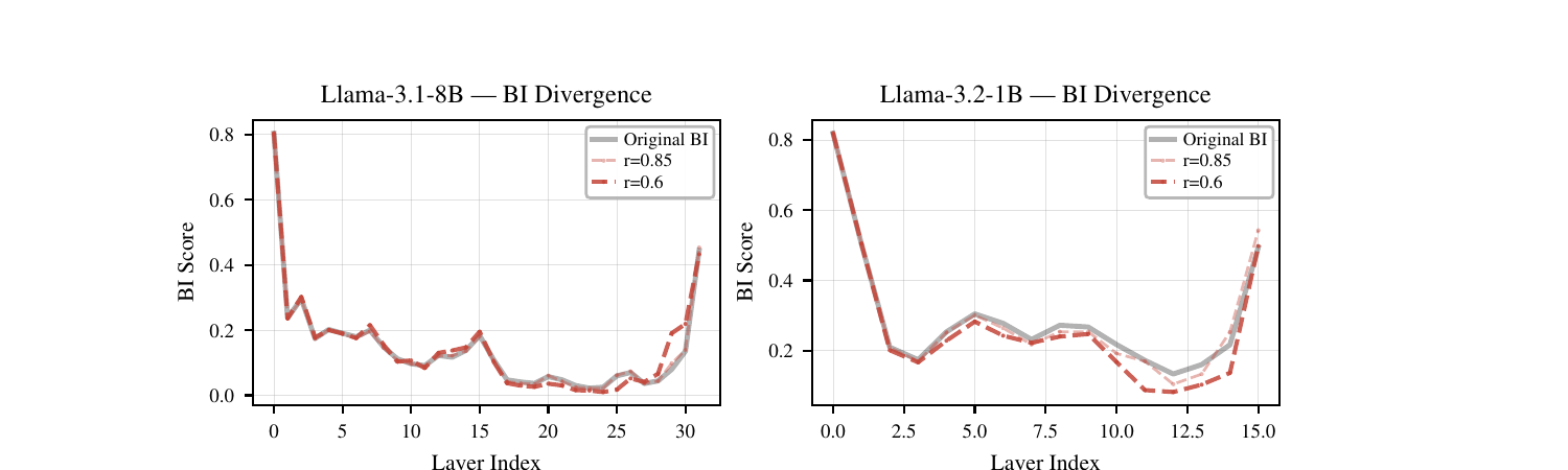
Figure 2 makes this concrete. For Llama-3.2-1B at rank ratio $r=0.85$ (i.e., 15% compression), layer 12’s BI score shifts from 0.13 (original) to 0.10 (post-compression) — the layer became less important than originally estimated, meaning the original allocation over-preserved it. Layer 15 shifts the opposite way: 0.49 → 0.54 — it became more important than estimated, meaning it was under-preserved. Both directions of error exist simultaneously, at different layers, and the pre-computed rank allocation has no way to know about either.

Together, these two drifts explain a structural blind spot in the entire “training-free joint decomposition” family: the compression decisions (both the reconstruction objective and the rank budget) are computed relative to a snapshot of the model that stops being accurate the moment compression begins.

The Proposed Fix: Two Training-Free, Pipeline-Compatible Corrections

The paper’s core contribution is two corrections, designed to be modular add-ons compatible with any existing training-free decomposition framework (they implement both on top of UniQL, currently the fastest SOTA joint-decomposition method).

Architecture / Pipeline Overview

flowchart TB
    subgraph Baseline["Baseline pipeline (e.g. UniQL / MoDeGPT)"]
        A1["Pass calibration data through ORIGINAL model once"] --> A2["Freeze activation stats + BI scores"]
        A2 --> A3["Compute layer rank ratios φ (once)"]
        A3 --> A4["Compress every layer using frozen stats + fixed φ"]
    end
    subgraph Corrected["This paper's corrected pipeline"]
        B1["Init φ from original model's BI scores"] --> B2["Round n = 1..N"]
        B2 --> B3["For each layer l (in order):<br/>compress layer l using CURRENT calibration x"]
        B3 --> B4["Forward pass through the just-compressed layer l<br/>to refresh x for layer l+1<br/>(Calibration Correction)"]
        B4 --> B3
        B3 --> B5["After full pass: recompute BI on compressed model,<br/>update φ via delta rule<br/>(Rank Allocation Correction)"]
        B5 --> B6{"φ converged?<br/>(divergence < ε)"}
        B6 -- no --> B2
        B6 -- yes --> B7["Return compressed model"]
    end

The left half of the diagram is what every prior training-free joint-decomposition method does: one calibration pass on the original model, one BI-score computation, one fixed rank budget, then compress everything using those frozen numbers. The right half is this paper’s proposal: interleave calibration refresh with compression (Correction 1), and wrap the whole thing in an outer iterative loop that re-estimates rank ratios on the compressed model and blends them back in (Correction 2).

Correction 1: Layer-by-Layer Compression with Calibration Correction

The fix for Drift #1 is almost embarrassingly simple once you see it: instead of collecting calibration activations for all layers in one pre-processing sweep through the original model, collect them layer by layer, interleaved with compression. Concretely: compress layer $l$, then immediately run a forward pass through the just-compressed layer $\hat M[l]$ (not the original layer!) to obtain the activations that will actually feed into layer $l+1$‘s calibration.

This transforms the reconstruction objectives from Equations (4) and (5) (using the original model’s activations $X$ throughout) into:

$$O = \min\left(\|WX - \hat W \hat X\|^2\right) \tag{8}$$ $$O = \min\Big(f(\|X; W_1, \cdots, W_k\|^2) - f(\|\hat X; \hat W_1, \cdots, \hat W_k\|)\Big)^2 \tag{9}$$

where $\hat X$ denotes activations produced by the already-compressed upstream layers, as opposed to $X$, the activations from the original, uncompressed upstream layers. Notice the objective is identical in form to Equations (4)/(5) — the only thing that changed is which activations you plug in. That’s why this correction is “free”: it requires no new machinery, no new hyperparameters (beyond what the base decomposition already needs), and virtually no additional compute overhead, since you were already going to run forward passes at some point to validate the compressed layer; you’re just doing it eagerly and reusing the result.

Why does this actually fix the accumulation problem? Because now, by construction, layer $l+1$‘s decomposition objective is computed against exactly what layer $l+1$ will see at inference time (since layer $l$ is already fixed/compressed by the time we get to $l+1$). There is no growing gap between “what calibration assumed” and “what the compressed model produces” — the calibration signal is always freshly derived from the actual, current state of the model. Drift #1, by design, cannot accumulate under this scheme because each layer’s calibration is re-derived at the moment it’s needed rather than inherited from a stale, pre-computed snapshot.

Correction 2: Iterative Compression with Rank Allocation Correction

Correction 1 fixes representation-level drift but does not touch the rank allocation vector $\phi$ — that’s still computed once, from the original model’s BI scores, before any compression starts. Correction 2 addresses this by wrapping the whole compression procedure in an outer loop of $N$ rounds, where each round: (a) fully compresses the model using the current $\phi$, (b) re-measures BI scores on the resulting compressed model, and (c) updates $\phi$ to better reflect the compressed model’s actual importance profile.

The update rule is inspired by the delta rule used in Gated Delta Networks (itself tracing back to the classic Widrow-Hoff learning rule):

$$\hat\phi_i^n = \phi_i + \mathrm{Pr}\left(\alpha \times \Delta_i^n,\ r_{\text{target}}\right) \tag{10}$$ $$\Delta_i^n = \frac{\mathrm{BI}_i^n - \mathrm{BI}_i}{\max_{l \in [1,L]}(|\mathrm{BI}_l^n - \mathrm{BI}_l|)}, \quad \forall i \in \{1,\cdots,L\} \tag{11}$$

Let’s unpack this term by term:

• $\mathrm{BI}_i$ is the original (pre-compression) Block Influence score for layer $i$, and $\mathrm{BI}_i^n$ is the BI score measured on the compressed model after round $n$. Their difference, $\mathrm{BI}_i^n - \mathrm{BI}_i$, is the raw drift signal: positive means the layer turned out to be more important than originally thought (should get more capacity), negative means it turned out less important (can afford more compression).
• The denominator $\max_{l}(|\mathrm{BI}_l^n - \mathrm{BI}_l|)$ is a global normalization — it rescales every layer’s drift by the single largest observed drift across all layers, so $\Delta_i^n \in [-1, 1]$. This keeps the correction magnitude comparable across models/layers with very different absolute BI scales.
• $\alpha \in [0,1]$ is a dampening coefficient. It plays exactly the role of a learning rate: $\alpha=1$ would apply the full measured drift immediately (risking overcorrection / oscillation, similar to an overly aggressive optimizer step), while a small $\alpha$ makes incremental, conservative adjustments. The paper explicitly draws this analogy to learning-rate scheduling in fine-tuning.
• $\mathrm{Pr}(\cdot, r_{\text{target}})$ is a projection function that maps the raw, damped drift signal back onto a valid rank-ratio vector that respects the global compression budget $r_{\text{target}}$ — i.e., after nudging individual layers up or down, the overall average compression ratio across the whole model must stay fixed at the target the user asked for. This is analogous to a constrained-optimization projection step (think projected gradient descent): you take a raw update, then project it back onto the feasible set (here, “the average retention ratio equals $r_{\text{target}}$”).
• Why add $\phi_i$ (the previous rank ratio) at all rather than replacing it outright with the newly measured BI-derived ratio? Because, as the paper argues, “each layer possesses unique information and task proficiency that should be preserved to some extent in relation to the original model despite the shifting layer importance distribution.” In other words: don’t throw away the calibration you already trust just because one BI measurement moved a bit; blend the new evidence in gradually. This is the same philosophy behind exponential moving averages or momentum terms in optimization — trust historical estimates somewhat, update incrementally rather than jumping straight to the newest noisy measurement.

Algorithm 1, Fully Unpacked

Here is the complete pseudocode from the paper, annotated line by line:

Algorithm 1: Iterative compression and calibration correction
Input:  Model M; calibration data x_in; target rank ratio r_target;
        dampening coefficient α
Output: Compressed model M_hat_n

1:  φ ← COMPUTE_LAYER_RATIOS(M, r_target)      # initial BI-based rank ratios,
                                                # computed once on the ORIGINAL model
2:  for n in {1, ..., N}:                      # outer loop: N refinement rounds
3:      x ← x_in                               # reset calibration input to the raw
                                                # calibration dataset for this round
4:      for l in {1, ..., |M|}:                # inner loop: walk through every layer
                                                # of the model IN ORDER (crucial: order
                                                # matters because each layer depends on
                                                # the previous layer's compressed output)
5:          M_hat_n[l] ← COMPRESS_LAYER(M[l], x, φ_l)
                                                # compress layer l using the CURRENT
                                                # calibration x and its assigned ratio φ_l
                                                # (this is a call into whatever base
                                                # decomposition method you're using --
                                                # e.g. UniQL's or MoDeGPT's per-module
                                                # compression routine)
6:          x ← M_hat_n[l](x)                  # <<< CALIBRATION CORRECTION >>>
                                                # forward the calibration data through the
                                                # layer we JUST compressed (not the
                                                # original layer!), producing the activations
                                                # that layer l+1 will actually see
7:      φ_hat ← UPDATE_LAYER_RATIOS(M_hat_n, r_target, φ, α)
                                                # <<< RANK ALLOCATION CORRECTION >>>
                                                # re-measure BI on the fully compressed
                                                # model M_hat_n, apply the delta rule
                                                # (Eq. 10-11), and project back onto the
                                                # r_target budget
8:      if DIV(φ, φ_hat) < ε:                  # convergence check: how much did the
                                                # rank-ratio vector change this round?
9:          break                              # if the change is below a small
                                                # threshold ε, we've converged --
                                                # stop early (saves compute)
10:     else:
11:         φ ← φ_hat                          # otherwise, adopt the updated ratios
                                                # and go around again with a NEW full
                                                # compression pass (line 3 resets x)
12: return M_hat_n

A few things worth calling out that aren’t obvious from a first skim:

1. Line 3 resets x at the top of every outer round. This means each round of the N-round loop performs a complete recompression of the model from scratch, layer by layer, using the (possibly updated) rank ratios $\phi$. It is not an incremental patch to a previously compressed model — it’s “compress the whole thing again, but smarter this time.” This has real cost implications discussed below.
2. Line 5-6 (the shaded “calibration correction” step) runs inside every round, not just the first. This means Correction 1 (calibration freshness) and Correction 2 (rank allocation refinement) are not mutually exclusive alternate modes — they compose naturally, since every full compression pass already benefits from fresh, layer-by-layer calibration regardless of which round of $N$ we’re on.
3. The exit condition (lines 8-9) is a divergence check on $\phi$ itself, not on downstream task accuracy. This is a pragmatic design choice: you don’t want to be running expensive downstream evaluations (e.g. LM-Eval Harness benchmarks) inside the compression loop just to decide when to stop — that would defeat the “training-free, cheap” premise of the whole approach. Instead, the algorithm uses a cheap, purely internal signal (has the rank allocation stabilized?) as a proxy for “has the pipeline converged enough that further rounds won’t help much.”

Design Choices, Alternatives, and Where They Break

(1) Why layer-by-layer calibration correction instead of a full end-to-end re-calibration after each round? An alternative design would be: compress the entire model once, then run a second full calibration pass through the entire compressed model to get fresh statistics for a second compression attempt (i.e., correct calibration only between rounds, not within a round). The paper’s chosen design corrects calibration within a single pass, at every layer boundary, which is strictly finer-grained. The advantage: within-pass correction eliminates the entire accumulation problem in a single compression round, rather than requiring multiple outer rounds just to chase down calibration drift. The cost: it couples the calibration-correction mechanism tightly to a sequential, layer-order traversal, which forecloses parallelizing compression across layers (you cannot compress layer 5 before layer 4 finishes, because layer 5’s calibration depends on layer 4’s compressed output). For models with hundreds of layers this sequential dependency could become a real wall-clock bottleneck, which the paper’s own timing numbers (Table 2, discussed below) partially confirm.

(2) Why a delta/EMA-style blended update for rank allocation instead of directly substituting the newly measured BI scores each round? The obvious alternative — just recompute $\phi$ from the current BI scores at the start of every round, ignoring the previous $\phi$ entirely — is simpler and has fewer hyperparameters ($\alpha$ wouldn’t be needed at all). The paper’s justification for the blended delta update is stability: BI scores measured after one round of compression are themselves noisy estimates (Figures 4 and 5 show the accuracy trajectory can oscillate across rounds rather than monotonically improve), so directly substituting a noisy new estimate for a previously reasonable one risks whiplashing the rank allocation back and forth. The dampened delta update is explicitly designed to prevent this oscillation, at the cost of an extra hyperparameter ($\alpha$) that the paper itself shows is model- and rank-dependent (their own ablations in Figures 4/5 show the sign of the best choice between $\alpha=0.01$ and $\alpha=0.05$ flips depending on the model and target rank ratio). This is a real practical downside: there is no universal $\alpha$ that works everywhere, and the paper does not offer an automated way to select $\alpha$ per deployment — it’s left as a manual grid-search hyperparameter (Appendix C.5 does exactly this grid search over $\alpha \in \{0.01, 0.05\}$ and $N \le 3$).

(3) Why is the exit criterion based on rank-ratio convergence rather than an accuracy proxy? As discussed above, using downstream accuracy as a stopping signal would require an evaluation harness inside the compression loop, undermining the “cheap, training-free” value proposition. The chosen alternative — stop when $\phi$ stabilizes — is cheap but has a subtle failure mode: $\phi$ can converge (stop changing) even though the underlying accuracy is still oscillating or hasn’t reached its best value for that model. Indeed, Figures 4 and 5 show accuracy trajectories that are non-monotonic across the very small number of rounds ($N \le 3$) the paper actually tests — meaning a $\phi$-based stopping rule could plausibly stop one round too early or one round too late relative to the accuracy-optimal point, and the paper has no mechanism to detect or correct for that mismatch.

(4) Why build the correction on top of UniQL specifically, rather than MoDeGPT? The paper is explicit about this: UniQL is roughly 2.5–5× faster to compress than MoDeGPT (Table 2) because it replaces MoDeGPT’s expensive pseudo-inverse-based Nyström approximation with a cheaper column-sorting/truncation approach. Since Correction 2 already multiplies the wall-clock cost of compression by (up to) $N$ rounds, building on the slower MoDeGPT baseline would have compounded that overhead — building on UniQL keeps total compression time in the tens-of-minutes range even with iterative refinement. The tradeoff: this choice ties the paper’s headline numbers to one specific base decomposition algorithm’s quirks (e.g. UniQL’s structural truncation granularity of multiples of 16 for attention weights and 128 for MLP weights), and it’s not obvious from the paper how much of the improvement would transfer if applied on top of a fundamentally different base method (e.g. a pruning-based or quantization-based pipeline) rather than another joint SVD decomposition method.

Experimental Results, Walked Through

Main Accuracy Table

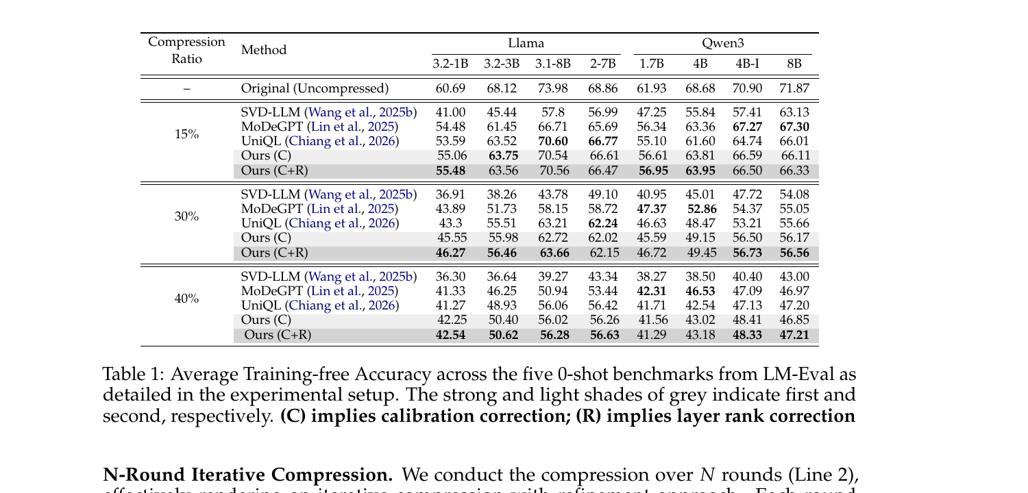
This is the paper’s core result table. A few observations worth drawing out beyond the headline “1-2.5pp improvement”:

• At the mildest compression level (15%), the corrections give modest but consistent gains on Llama models (e.g. Llama-3.2-3B: UniQL 63.52 → Ours (C+R) 63.56, essentially a tie; Llama-3.2-1B: 53.59 → 55.48, a solid +1.9pp gain). The gains generally widen as compression gets more aggressive — at 40% compression, Llama-3.2-1B goes from UniQL’s 41.27 to 42.54 with (C+R), and Llama-3.2-3B from 48.93 to 50.62, a full +1.7pp gain. This directionally makes sense: at low compression the model has plenty of slack, so calibration/rank drift is a second-order effect; at aggressive compression, every bit of misallocated capacity or stale calibration signal actively costs accuracy.
• The Qwen3 family tells a more nuanced story. At 15% compression, UniQL and the paper’s methods are close, but MoDeGPT actually wins outright on Qwen3-4B (67.27 vs the paper’s best 66.59) and Qwen3-4B-Instruct (67.30 vs 66.50). This is one of the honest, non-cherry-picked data points in the paper — the authors don’t hide it, and they discuss it directly in Section 4.3 (“For the Qwen3 family, MoDeGPT achieves the smallest gap”). We’ll come back to why this matters in the critical analysis section.
• Comparing (C) alone versus (C+R): the rank allocation correction (R) gives a smaller, more inconsistent boost on top of calibration correction (C) alone — sometimes it helps (Llama-3.2-1B at 30%: 45.55 → 46.27), sometimes it’s roughly neutral or slightly negative (Qwen3-1.7B at 15%: 56.61 → 56.95, a small gain; but at 30%: 45.59 → 46.72, also a gain — so in this table R generally helps, but the margin is thin and inconsistent in sign across model×rate combinations elsewhere in the paper’s appendix tables).

Average Gap From Best — A Smart Aggregate Metric

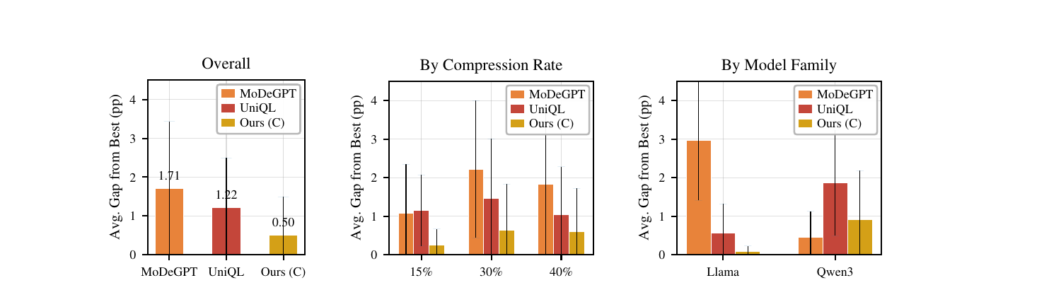
Rather than eyeballing dozens of individual numbers in Table 1, the paper introduces a clean aggregate: for each (model, compression rate) configuration, compute how far each method’s accuracy is below the best accuracy achieved by any method in that configuration, then average this gap across all configurations. Lower is better; 0 means “always the best.” The overall panel shows MoDeGPT averaging 1.71pp behind the best, UniQL 1.22pp behind, and the paper’s calibration correction only 0.50pp behind — a genuine >2x improvement in closeness-to-oracle over the next-best baseline. The “by model family” panel is the most informative slice: it visually confirms the Llama/Qwen3 asymmetry noted above — the paper’s method has an almost-zero gap on Llama models but a non-trivial ~1pp gap on Qwen3, while MoDeGPT is the mirror image (large gap on Llama, small gap on Qwen3).

Does Rank Allocation Correction Actually Help Monotonically? Not Always.

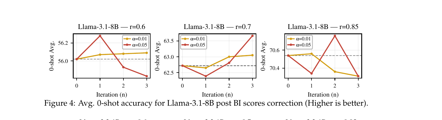
This is one of the more scientifically honest figures in the paper. Look closely at the middle and right panels for Llama-3.1-8B ($r=0.7$ and $r=0.85$): the accuracy curves are not monotonically increasing with more refinement rounds. For $r=0.85$, $\alpha=0.01$: accuracy actually goes up then down then up again across rounds 0→1→2→3. For Llama-3.2-1B at $r=0.6$ (second row, left panel), $\alpha=0.05$ actively hurts at round 2 before recovering at round 3. This tells you the iterative refinement process is not a well-behaved, convergent optimization in the classical sense — it’s closer to a noisy local search that sometimes helps and sometimes needs several rounds before the noise averages out favorably. The paper’s stated takeaway (“a small number of rounds, N∈[1,3] can be sufficient”) is defensible as an empirical average, but it also means that for any specific deployment you don’t know in advance whether round 1, 2, or 3 will be your best checkpoint — you’d need to actually evaluate multiple rounds and pick the best one after the fact, which reintroduces exactly the kind of “run an eval harness during compression” overhead the training-free philosophy was trying to avoid.

Compute Cost: The Iterative Loop Isn’t Free

Table 2 in the paper (reproduced inline in the method-discussion figure above) reports wall-clock compression time: MoDeGPT takes 3h1m for Llama-3.1-8B, UniQL takes just 19 minutes, and the paper’s calibration-corrected method (a single round, no rank correction) takes 35 minutes — roughly 1.8x slower than plain UniQL. This makes sense: the layer-by-layer calibration correction requires a fresh forward pass through each just-compressed layer, which is extra compute that UniQL’s original one-shot calibration approach didn’t need. Critically, this 35-minute number is for a single compression round without the outer $N$-round rank-allocation refinement — if you run $N=3$ rounds of the full (C+R) pipeline, the total time would scale roughly linearly with $N$ (each round redoes the entire layer-by-layer compression from scratch per Line 3 of Algorithm 1), meaning the full (C+R) treatment for an 8B model could plausibly approach 1.5-2 hours or more, a meaningfully different cost profile from UniQL’s 19-minute baseline, and one the paper doesn’t report a headline number for.

Ablations: Repeated Seeds and Scaling to 32B

Table 3 (seeded repeats) shows the improvements are not a statistical fluke of a single lucky run — repeating with 3 additional seeds at 40% compression on Llama-3.2-1B and 3.2-3B, the (C) and (C+R) methods consistently edge out UniQL, with small variances (e.g. Llama-3.2-3B WikiText-2 PPL: UniQL 70.85±1.28 vs Ours (C+R) 60.68±3.89 — notice the higher variance for the corrected method, an honest signal that the correction, while better on average, is somewhat less stable run-to-run).

Table 4 (scaling to Qwen2.5-32B) delivers the paper’s most important caveat, and to their credit they report it plainly: at 32B scale, pure calibration correction (C) does not help and can even hurt (0-shot avg drops from 59.84 to 57.42, MMLU from 32.40 to 27.20) relative to plain UniQL. Only the rank allocation correction (R), applied directly on top of the uncompressed UniQL baseline (skipping calibration correction), shows a modest gain (+0.3pp 0-shot avg, +0.05 MMLU at best settings). The paper’s own interpretation: “larger models are generally more stable and resilient to calibration drifts and layer sensitivity shifts” — meaning the entire motivating premise of the paper (drift accumulates and matters) weakens as models get bigger, which is precisely the regime (frontier-scale models) where compression research arguably matters most for real deployment cost savings.

A Closer Look: Why Qwen3 Resists the Correction

Since the Qwen3-vs-Llama asymmetry keeps resurfacing across every figure in this paper, it’s worth digging into the specific mechanism the authors identify, because it reveals something interesting about how architectural choices interact with importance-based rank allocation.

Recall the Block Influence score: $\mathrm{BI}_i = 1 - \mathrm{CosSim}(X_i, X_{i+1})$. A layer with BI close to 1 changes its input activation direction dramatically; a layer with BI close to 0 leaves its input essentially untouched (in terms of direction). The paper’s Appendix Table 5 reports first- and last-layer BI scores for the Qwen3 family at two compression levels:

Model	15% comp. first layer	15% comp. last layer	40% comp. first layer	40% comp. last layer
Qwen3-1.7B	0.9999	0.9926	0.9990	0.9802
Qwen3-4B	0.9999	0.9318	0.9998	0.8181
Qwen3-8B	0.9995	0.8928	0.9988	0.7140

Every single one of these numbers is close to the ceiling of 1.0. Compare this to Llama models, where BI scores in Figures 2, 8, and 9 range broadly from near 0 (many middle layers) up to roughly 0.5-0.8 at the extremes. When you push these Qwen3 BI values through the temperature-scaled softmax in Equation (7),

$$\phi = L \times r_{\text{target}} \times \text{Softmax}\left(\frac{-\text{scores}}{\tau}\right),$$

the softmax has almost no meaningful spread to work with for the first and last layers — they are saturated near the top of the importance ranking regardless of what happens elsewhere in the network, so the allocator assigns them retention ratios close to full rank almost automatically, leaving comparatively little room for the allocation algorithm’s relative judgments about middle layers to matter. The paper’s own hypothesis for why Qwen3 saturates this way is architectural: Qwen3’s tokenizer uses an unusually large 151k-token vocabulary (roughly 4x Llama-3’s ~32k-128k vocabulary depending on version), meaning the embedding/first-layer transformation and the final unembedding/last-layer transformation both have to route information through a much higher-dimensional discrete symbol space, plausibly making these two boundary layers do disproportionately more “transformation work” per forward pass regardless of compression state.

The deeper implication for this paper’s Correction 2 (rank allocation correction) is that when BI scores are already pinned near a hard ceiling both before and after compression, there is very little drift signal for the delta update rule (Equations 10-11) to actually correct — $\Delta_i^n$ is computed from the difference between pre- and post-compression BI, and if both numbers are stuck near 0.99+, that difference is necessarily small no matter how much the underlying weight distributions have actually shifted. This offers a mechanistic explanation for why the rank-allocation correction specifically underperforms on Qwen3 relative to Llama: it’s not that the underlying drift phenomenon doesn’t occur, but that the BI-score-based measurement instrument the correction depends on has poor sensitivity in the regime Qwen3’s architecture happens to occupy.

Limitations

The authors are commendably upfront about several limitations in their own dedicated section:

• Model size ceiling. All main experiments are on models ≤8B parameters (with one 32B ablation that shows weaker results for the flagship calibration correction). The paper explicitly flags “extensive testing on larger model sizes (>8B models)” as unresolved.
• Compression rate ceiling. All experiments stop at 40% compression; the paper flags “aggressive compression ratios (<50% retention)” as unexplored territory. Since drift accumulation should, if anything, get worse at more extreme compression (per Figure 1’s own trend line), this is a real gap — we don’t know if the corrections still help, help more, or start to break down beyond 50%.
• Architecture coverage. Only standard dense transformer architectures (Llama, Qwen3) are tested. The paper explicitly notes hybrid architectures and state space models (e.g. Mamba-style) as future work, and these architectures have fundamentally different activation dynamics that BI-score-based importance measures were never validated against.
• Dependence on a single importance metric. All rank allocation logic depends on the Block Influence (BI) score specifically. The paper acknowledges “the resulting rank allocation remains conditioned on the selected scoring mechanism” and explicitly leaves robustness to alternative importance metrics as future work.

Critical Analysis

Weaknesses and flaws specific to this paper

1. The convergence criterion (rank-ratio divergence) is decoupled from the actual quantity you care about (accuracy), and the paper’s own figures show this can matter. As discussed above, Figures 4-5 show non-monotonic accuracy trajectories across rounds, meaning stopping when $\phi$ stabilizes is not guaranteed to coincide with the best-accuracy round. A more rigorous treatment would at minimum report how often the $\phi$-convergence stopping point matches the empirically best round in their own experiments — this analysis is conspicuously absent.
2. The hyperparameter sensitivity of $\alpha$ is real but under-addressed. The paper shows (their own Figures 4/5, Tables 10/11 in the appendix) that the sign of whether $\alpha=0.01$ or $\alpha=0.05$ is preferable flips depending on model and rank ratio, and Table 11 even shows the average effect of rank correction can be negative for some model groupings at $N=1$ (e.g. Llama-3.2-1B/3B group: −0.10 average change at $\alpha$-average, meaning rank correction on average hurt accuracy for that group at a single round). This is a meaningfully understated point in the main text abstract’s “1-2.5pp improvement” headline, which obscures that the rank-correction component specifically is not reliably positive.
3. The wall-clock cost tradeoff for the full (C+R) pipeline is never reported as a single headline number. Table 2 only reports timing for calibration correction (C) alone, not for the full iterative (C+R) pipeline at $N=3$ rounds, which per Algorithm 1’s structure should cost roughly 3x the single-round number. This is a significant omission for a paper whose entire premise is “training-free, cheap compression” — the actual cost of getting the full advertised accuracy gain (which requires C+R, not just C, per Table 1) is materially higher than the reported 35-minute / 2.5-5x-faster-than-MoDeGPT headline suggests.

Limitations the authors understate or omit

1. The Qwen3 weakness is more than an isolated anomaly — it may reflect a structural mismatch with the BI score itself. The paper’s own Appendix analysis (Table 5) reveals why Qwen3 is different: its first and last layers carry disproportionately high BI scores (up to 0.9999 at the first layer), which the paper attributes to Qwen3’s unusually large 151k vocabulary. This means the BI-score-based rank allocation heuristic — the very mechanism Correction 2 is built around — behaves qualitatively differently across model families for reasons that have nothing to do with the drift phenomenon the paper is trying to fix. This is a much deeper concern than “Qwen3 happens to benefit less”; it suggests the underlying importance metric itself may need architecture-specific calibration, a possibility the paper mentions only in a single paragraph buried in the appendix rather than surfacing as a first-class limitation in the main text.
2. No error bars or statistical significance testing on the headline Table 1 results, aside from the separate seeded-repeat ablation on only two small Llama models. Given that Table 3’s seeded repeats show non-trivial standard deviations (e.g. ±3.89 for a PPL metric), it’s plausible that some of the smaller accuracy gaps reported as wins in Table 1 for the 8 main models (which use a single seed each) fall within noise, but we cannot tell from the paper as written.
3. The paper doesn’t discuss the interaction between the sequential, layer-order dependency introduced by calibration correction and modern distributed/multi-GPU compression workflows. Because Correction 1 requires each layer’s calibration to depend on the immediately preceding layer’s compressed output, this inherently serializes what could otherwise be a more parallelizable per-layer compression procedure. For very large models where compression itself needs to be distributed across multiple devices, this sequential coupling could be a meaningfully larger practical cost than the wall-clock numbers on a single 48GB GPU suggest.

Concrete, specific improvement suggestions

1. Report a $\phi$-convergence-vs-accuracy-optimal-round correlation analysis. Given the non-monotonic accuracy trajectories already visible in Figures 4-5, the paper should directly measure, across all their (model, rank-ratio, $\alpha$) sweep results, how often the round selected by the $\phi$-divergence stopping criterion matches (or is close to) the empirically best-accuracy round. If the correlation is weak, this motivates a cheap accuracy-aware or hybrid stopping criterion (e.g., a lightweight proxy metric computed on a tiny held-out validation slice, rather than a full benchmark suite) as a natural follow-up.
2. Provide a single headline wall-clock number for the complete (C+R) pipeline at the $N$ that achieves the reported Table 1 numbers, not just for calibration correction alone. Compression-time-vs-accuracy is a genuine Pareto tradeoff that practitioners need to reason about, and burying the full-pipeline cost in an implicit “roughly Nx the reported (C) number” leaves readers to do the multiplication themselves (or worse, not realize they need to).
3. Investigate an architecture-aware or learned alternative to raw BI scores for rank allocation, specifically to address the demonstrated Qwen3 first/last-layer BI saturation issue (Table 5) — for instance, normalizing BI scores relative to a per-architecture baseline distribution, or capping/floor-ing extreme BI values before they dominate the softmax-based ratio derivation (Equation 7 from Section 2.3), rather than leaving this as an unexplained anomaly in an appendix table.
4. Extend the ablation matrix to include at least one hybrid or state-space architecture and one >30% compression rate with the flagship model size (8B+), even at reduced scope (e.g., a single model, single seed), specifically because the paper’s own trend lines (Figure 1: NMSE keeps climbing past 40%; Table 4: 32B weakens the calibration-correction case) both point toward the untested regimes being exactly where the method’s behavior is least predictable from the reported data.

A Worked Numerical Example

Abstractions like Equations (10)-(11) are easier to internalize with concrete numbers. Suppose we’re compressing a small 4-layer toy model to $r_{\text{target}} = 0.7$ (i.e., retain 70% of parameters on average), and after the first compression round we measure the following BI scores:

Layer $i$	Original $\mathrm{BI}_i$	Post-compression $\mathrm{BI}_i^1$	$\mathrm{BI}_i^1 - \mathrm{BI}_i$
1	0.10	0.10	0.00
2	0.45	0.38	−0.07
3	0.60	0.72	+0.12
4	0.20	0.20	0.00

The largest absolute drift across all layers is $|0.12| = 0.12$ (layer 3), so the normalization denominator in Equation (11) is $0.12$. This gives:

$$\Delta_1^1 = \frac{0.00}{0.12} = 0.00, \quad \Delta_2^1 = \frac{-0.07}{0.12} \approx -0.583, \quad \Delta_3^1 = \frac{0.12}{0.12} = 1.00, \quad \Delta_4^1 = \frac{0.00}{0.12} = 0.00$$

Now apply the dampening coefficient, say $\alpha = 0.05$: the raw (pre-projection) nudges are $\alpha \times \Delta_i^1 = \{0, -0.029, 0.05, 0\}$. Layer 2 gets nudged down (it turned out less important than originally thought — its BI score dropped after compression, so it can absorb slightly more compression next round), and layer 3 gets nudged up (it turned out more important — its BI score actually rose after compression, meaning it should be preserved more carefully). Layers 1 and 4 are untouched because their BI scores didn’t drift at all. Finally, $\mathrm{Pr}(\cdot, r_{\text{target}}=0.7)$ takes these four raw nudges added to the previous $\phi$ vector and rescales/clips them so the average retention ratio across all four layers still equals exactly 0.7 — for instance, if layer 3’s nudge alone would push the average above 0.7, the projection step redistributes some of that increase as a small compensating decrease elsewhere. This little example captures the entire mechanism: measure how the model’s actual behavior changed, distill that into a relative per-layer signal, dampen it so no single measurement causes an overcorrection, and always snap back to the overall budget the deployment target requires.

How This Compares in Practice to Just Running More Calibration Samples

A natural question a practitioner might ask: instead of this whole layer-by-layer, iterative-refinement apparatus, why not simply throw more calibration data at the standard one-shot pipeline (e.g., 1024 samples instead of 128) to get a more robust initial estimate? The paper doesn’t run this specific ablation directly, but its own framing lets us reason about why more calibration data alone would not fix the problem: the drift the paper documents is not a sampling noise problem (where more samples would reduce variance in the statistics) — it’s a distributional mismatch problem (the calibration activations are computed against a model state, the original uncompressed weights, that no longer exists once compression starts). Adding more calibration samples would give you a more precise estimate of the wrong target (the original model’s activation statistics), not a correction toward the right target (the actual compressed model’s activation statistics). This is analogous to the difference between reducing variance and reducing bias in a statistical estimator: more data shrinks variance, but only fixing the underlying assumption (in this case, recalibrating against the actually-compressed layers) removes the systematic bias captured by the paper’s NMSE curves in Figure 1.

Synergy With Post-Hoc Correction: The EoRA Experiment

One appendix result deserves more attention than it gets in the main text: the paper’s investigation of whether its correction mechanisms compose with EoRA, a separate, post-hoc error-compensation technique. It’s worth being precise about what EoRA actually is, since the distinction from this paper’s approach is instructive. EoRA adds a parallel low-rank residual path $R_{\text{EoRA}}(\cdot)$ after compression is complete, specifically trained (via a small amount of additional optimization, unlike the fully training-free main pipeline) to approximate the residual error $\Delta W = W_{\text{comp}} - W_{\text{orig}}$ that compression introduced. Conceptually it’s similar to how a LoRA adapter is bolted onto a frozen base model to recover task performance — except here the “task” being recovered is simply matching the original, uncompressed model’s behavior as closely as possible.

Applying EoRA naively per weight matrix doesn’t work cleanly with joint/modular decomposition methods like UniQL, because joint decomposition slices channel dimensions jointly across multiple matrices in a module, so the compressed and original weight matrices no longer even have matching shapes at the individual weight level — you cannot directly compute $W_{\text{comp}} - W_{\text{orig}}$ elementwise. The paper’s workaround is to apply EoRA at the block level instead: define the residual at the module’s output rather than at any individual weight, $\Delta M = M_{\text{comp}}(x) - M_{\text{orig}}(x)$, which sidesteps the shape-mismatch problem because module outputs (not intermediate weight shapes) are guaranteed to match dimensionality. The corrected forward pass becomes

$$x_{\text{out}} = M_{\text{comp}}(x) + \eta \, R_{\text{EoRA}}(x),$$

where $\eta$ is an extra dampening coefficient (set to 0.1 in the paper’s experiments) introduced specifically to prevent overcorrection when stacking two independent correction mechanisms (this paper’s calibration/rank correction, plus EoRA’s residual path) on top of each other — a sensible defensive design choice, since two correction signals derived from related but not identical error sources could otherwise double-count some of the same error and overshoot.

The result (Table 15 in the paper): EoRA provides an additional +0.41 point average improvement on top of whatever base configuration (UniQL, Ours (C), or Ours (C+R)) it’s layered onto, and critically, the relative ordering between configurations is preserved after adding EoRA — whichever correction was best before EoRA remains best after. The paper interprets this as evidence that its in-compression corrections and EoRA’s post-hoc correction are addressing genuinely distinct error sources (calibration/rank drift during compression versus residual weight error after compression is fixed), so their benefits stack rather than substitute for each other. This is a meaningful practical takeaway for anyone deploying this method: the calibration/rank corrections and EoRA are not competing alternatives, they are complementary layers in a compression stack, and a production pipeline aiming for maximum accuracy at a given compression budget should likely use both together rather than picking just one.

Reproducibility Notes

The paper builds directly on the open-source UniQL implementation, and all baseline methods (SVD-LLM, MoDeGPT, UniQL) are themselves open-source, which is a meaningfully reproducibility-friendly starting point. Key experimental settings that would need to be matched for reproduction: 128 WikiText-2 samples for layer ratio estimation, 128 Alpaca samples for layer sorting/compression, BF16 precision, evaluation on NVIDIA RTX 6000 Ada GPUs (48GB), and the five LM-Eval Harness 0-shot tasks (PiQA, Winogrande, Arc-Easy, Arc-Challenge, Hellaswag) with normalized accuracy for Arc-Challenge and Hellaswag. The specific values of $\alpha \in \{0.01, 0.05\}$ and $N \le 3$ used in the main experiments are reported, but as discussed above, the paper does not give a principled recipe for choosing these per new model/rank-ratio combination — a practitioner reproducing this work on a new model family would need to run their own grid search analogous to Appendix C.5.

Where This Sits in the Low-Rank Compression Landscape

This paper occupies a specific, fairly narrow niche within the broader low-rank LLM compression literature: it is not a new decomposition algorithm (unlike SVD-LLM, MoDeGPT, or UniQL), but rather a correction layer that sits on top of an existing decomposition algorithm. This positions it closer in spirit to error-correction techniques from the quantization literature (e.g. GPTQ’s sequential error-compensation update rule, which similarly propagates a corrected residual to not-yet-quantized weights) than to the decomposition methods it’s evaluated against. Indeed, the paper explicitly acknowledges this connection, noting that “recent Post-Training Quantization (PTQ) methods introduced a similar correction philosophy” and that they are “generaliz[ing] the concept to be compatible with training-free low-rank decomposition frameworks.” The paper also explores synergy with EoRA (a post-hoc, parallel low-rank residual-path correction technique, conceptually related to LoRA-style adapters bolted on after compression) and finds the two corrections stack additively rather than being redundant — evidence that “corrections during compression” and “corrections after compression via an added adapter path” are addressing genuinely different error sources.

The Perplexity Numbers Tell a Consistent Story Too

Beyond the 0-shot accuracy tables discussed above, the paper’s Appendix C reports WikiText-2 and C4 perplexity (PPL) results comparing MoDeGPT against the calibration-corrected method (Tables 12-13 in the paper). Perplexity is a useful complementary signal because it’s a direct, task-agnostic measure of how well the compressed model’s output distribution matches the original language modeling objective, unlike downstream accuracy which can be noisy for small benchmark sets. At 40% compression, the pattern is striking and consistent with everything else in the paper: on WikiText-2, Llama-3.2-1B improves from MoDeGPT’s 44.21 PPL to the corrected method’s 41.70 (lower is better, so this is a meaningful win), and Qwen3-4B improves from 38.49 to 32.29 — a large relative gain. But at 15% compression, the differences shrink to near-parity (e.g., Llama-3.1-8B: 7.80 vs 7.80, exactly tied), reinforcing the pattern already visible in the accuracy tables: the correction’s value proposition scales with how aggressively you’re compressing, because that’s precisely when calibration and rank-allocation drift have had the most opportunity to accumulate. The C4 perplexity table (Table 13) tells largely the same story, with one interesting wrinkle: at 30% compression, a few configurations (e.g. Llama-3.2-3B: 30.33 vs 30.15, essentially tied but MoDeGPT technically better on Llama-3.1-8B at 23.99 vs 23.99) show the calibration correction providing negligible or even slightly negative benefit relative to MoDeGPT specifically — a reminder that MoDeGPT’s much more expensive pseudo-inverse-based reconstruction is not without merit; it is simply far slower (recall Table 2’s 3-hour compression time for an 8B model), and the corrected UniQL-based approach is trying to close that quality gap cheaply rather than definitively surpassing MoDeGPT everywhere.

Conclusion

This paper’s central contribution isn’t a flashier decomposition algorithm — it’s a careful diagnosis of a subtle, previously under-examined failure mode in an entire family of training-free low-rank compression pipelines, backed by clean NMSE and BI-divergence measurements that make the problem concrete and visualizable (Figures 1 and 2 alone are worth internalizing even if you never use this exact correction). The two proposed corrections are elegant in that they require no new training, minimal new machinery, and are drop-in compatible with existing SOTA pipelines. But the honest headline is nuanced: calibration correction is a robust, close-to-free win at small-to-medium model scales and moderate compression rates; rank allocation correction is a real but less reliable, hyperparameter-sensitive add-on; and both corrections’ value proposition measurably weakens exactly at the frontier-scale regime (32B+ parameters) where compression matters most in practice. If you’re building a training-free low-rank compression pipeline for models in the 1-8B range at 15-40% compression, this correction is very likely worth adopting on top of your existing UniQL/MoDeGPT-style base method. If you’re compressing frontier-scale models, treat the paper’s own Table 4 result as the more relevant data point than the flashier headline numbers.