ZeroLock: Breaking Update Locking in Pipeline-Parallel LLM Fine-Tuning

Review date: 2026-08-13 Author: Zhongzhu Zhou Paper reviewed: ZeroLock: Concurrent Memory-Efficient LLM Training via Modular Update Decoupling Paper authors: Wentao Dai, Xuanran Li, Yuxiang Zhang, Ming Tang, Chao Huang (Southern University of Science and Technology; Montclair State University) arXiv: 2608.07974 Venue/Status: Preprint (cs.LG), August 2026

1. Why pipeline-parallel fine-tuning still has a bubble problem

If you have ever tried to fine-tune a multi-billion-parameter LLM on a handful of edge GPUs, or worse, on a cluster of Android phones, you have run into the same wall: the model does not fit on one device, so you have to split it — and every way of splitting it that keeps standard backpropagation (BP) intact still leaves you with either idle compute (“bubbles”) or wasted memory (activations that have to be kept around far longer than you would like). ZeroLock is a systems-and-theory paper that attacks this problem at the algorithm level rather than the scheduling level: instead of finding a cleverer way to schedule BP’s forward/backward passes across pipeline stages, it asks whether you can replace BP itself, chunk by chunk, with something that does not need the whole chain to be intact before any stage can update.

This is a genuinely different lever than most pipeline-parallelism papers pull. GPipe, 1F1B, PipeDream, Zero-Bubble, and dozens of scheduling-focused follow-ups all keep the same computational graph — one long chain of forward operations feeding into one long chain of backward operations, glued together by the chain rule — and try to interleave, reorder, or overlap pieces of that chain across devices to shrink bubbles and reduce staleness. ZeroLock instead breaks the chain itself: each pipeline stage gets its own local loss function and updates its own parameters independently, using only the forward output of its upstream neighbor. No gradients ever cross a stage boundary. This single design choice is what eliminates both the throughput bottleneck (no waiting for downstream backward passes to finish) and the memory bottleneck (no need to retain activations until the whole chain’s backward pass completes) simultaneously, and it lets the paper build an actual working system that runs on both NVIDIA GPUs and unmodified Android phones.

Before diving into how ZeroLock does this, it’s worth spending real time on the background that makes the paper’s design choices legible: what “update locking” actually means mechanically, why previous BP-free approaches have not been adopted for LLM fine-tuning at the systems level, and what specifically was missing from the theory of local-objective training that this paper had to supply.

Prerequisites: what you need to know before diving in

Pipeline parallelism and stages. When a model is too large to fit on one device, one option is pipeline parallelism: partition the model’s layers into $K$ consecutive chunks, assign each chunk to a device (a “stage”), and feed micro-batches through the chain of stages like an assembly line. Device $k$ runs the forward pass for chunk $k$, hands its output (the “hidden state”) to device $k+1$, and so on until the last stage produces a loss; then gradients flow backward through the same chain, in reverse. This is efficient in principle — each device holds a much smaller slice of the model — but naively running micro-batches one at a time leaves most devices idle most of the time, since device $k$ cannot start processing micro-batch $i+1$ until it has finished forwarding micro-batch $i$ through every downstream device and received the corresponding backward signal.

GPipe, 1F1B, and PipeDream: three ways to fight bubbles without breaking BP. GPipe processes all forward passes of a logical batch before running any backward pass, so bubbles are large but the code is simple and fully synchronous. 1F1B (one-forward-one-backward) interleaves forward and backward computation within a batch, so a device can start its backward pass for micro-batch $i$ as soon as it is available rather than waiting for every micro-batch’s forward pass to finish first — this shrinks the “pipeline fill” bubble but still flushes the pipeline (drains all in-flight micro-batches) before the shared optimizer step, so update consistency is maintained at the cost of periodic idle time. PipeDream builds on 1F1B and removes the flush by allowing forward and backward passes from different update windows to overlap, using “weight stashing” — keeping multiple versions of the parameters around so that a backward pass always sees the exact parameter version that was used for its corresponding forward pass. This further raises utilization but at the cost of storing multiple weight snapshots, and more importantly for this paper’s argument, none of GPipe, 1F1B, or PipeDream change what the paper calls update locking: whatever the schedule, every stage’s parameter update still depends on completing a full round trip through every downstream stage’s forward and backward computation, because that is what the chain rule requires when there is one shared loss at the end of the chain.

Update locking, made concrete. Formally, if the model computes $h_k = f_k(h_{k-1}; W_k)$ for chunk $k$ (with $h_0$ the input embedding and $h_K$ feeding the final loss), then updating $W_k$ requires $\partial \mathcal{L}/\partial W_k$, which by the chain rule requires $\partial \mathcal{L}/\partial h_k$, which in turn requires the entire downstream chain from $h_k$ through $h_K$ to have both been computed forward and had its backward pass completed. This means:

• Throughput bottleneck: an upstream stage (say $S_0$) must wait for every downstream stage ($S_1$, $S_2$, …) to finish its own backward pass before $S_0$‘s backward pass — and hence $S_0$‘s update — can proceed. Scheduling tricks can shrink the resulting bubbles but cannot make them disappear, because the dependency, not merely the scheduling, is the bottleneck.
• Memory bottleneck: an upstream stage has to keep its activations (the intermediate tensors it computed on the forward pass) alive in memory until its own backward pass runs — which, per the point above, cannot happen until every downstream stage’s backward pass has finished. This means upstream stages hold onto memory far longer than they “need” to in a purely local sense, and the paper’s Fig. 1 visualizes this directly: at a given time slot, stage $S_0$ under a BP baseline might be holding three micro-batches’ worth of activations ($A_1$–$A_3$) simultaneously, purely because it is waiting on downstream stages, whereas an update-decoupled scheme only needs to hold the one activation set actually in use.

BP-free training: the two existing families, and why neither had been made to work for LLM pipeline fine-tuning at the systems level. The paper organizes prior BP-free work into two categories. Backward gradient estimation methods (direct feedback alignment, zeroth-order optimization à la MeZO) avoid the chain rule by estimating gradients through alternative means — propagating target errors directly to every layer, or perturbing parameters and using loss differences as a gradient proxy — but both tend to either degrade accuracy substantially on complex tasks or add prohibitive compute overhead (zeroth-order methods in particular need many forward-pass evaluations per update to get a usable gradient estimate). Objective reconstruction methods instead give each chunk its own local objective so its update never needs a signal from downstream at all — NoProp treats layers as independent denoising units, predictive coding alternates local prediction-error minimization with local weight updates, and depth-progressive monotonic learning (the paper’s own most direct ancestor) equips each layer of a classifier with an independent local loss. This family is the more promising one for LLM fine-tuning because it tends to preserve accuracy reasonably well, but — and this is the paper’s key positioning claim — nobody had (a) adapted it to LLM-specific ingredients like LoRA and autoregressive token-level losses, (b) proven convergence for the resulting algorithm under an arbitrary number of chunks (an earlier paper, LoPT, analyzed only the two-chunk case), or (c) actually built a deployable multi-GPU-or-multi-phone system around it with the runtime machinery (buffering, failure recovery, RPC-free hidden-state exchange) that real pipeline training needs. ZeroLock’s contribution is squarely aimed at filling exactly these three gaps — which the paper phrases as three research questions, Q1 (how to fine-tune with local objectives), Q2 (does modular decoupling hurt convergence), and Q3 (how to build a real system) — and the rest of the paper is organized around answering each in turn.

LoRA, briefly, since ZeroLock is built on top of it. Low-Rank Adaptation freezes the pretrained weight matrix $w_l$ of layer $l$ and learns a low-rank update $\Delta w_l = B_l A_l$, where $B_l \in \mathbb{R}^{d_3 \times d_2}$ and $A_l \in \mathbb{R}^{d_1 \times d_3}$ with rank $d_3 \ll \min(d_1, d_2)$. Only $A_l$ and $B_l$ are trained; the base weights $w_l$ never change. This matters for ZeroLock specifically because it keeps the trainable-parameter footprint of each pipeline stage small, which is a precondition for fine-tuning being feasible on memory-constrained edge devices (including phones) at all.

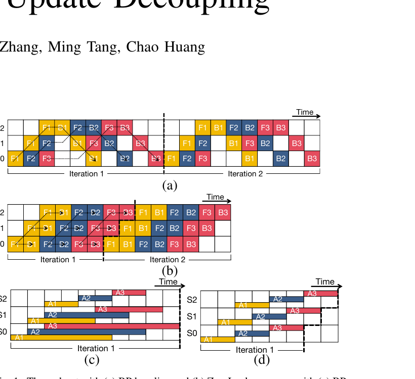
Fig. 1 is worth staring at for a moment, because it is the single image that makes the paper’s entire pitch legible. In the BP timeline (a), notice how stage $S_0$‘s forward passes $F_1, F_2, F_3$ all complete early, but its backward passes $B_1, B_2, B_3$ are pushed out in time, each one waiting for the corresponding backward pass to finish on $S_1$ and $S_2$ first — the diagonal dependency arrows sketched in the figure trace exactly this chain-rule dependency. In the ZeroLock timeline (b), each stage’s backward pass follows immediately after its own forward pass, with no dependency on downstream stages at all — the schedule becomes fully local. The memory panels (c) and (d) show the mechanical consequence: under BP, $S_0$ has to keep three micro-batches’ worth of activations alive at once (the overlapping colored bars), because the earliest one cannot be freed until its backward pass eventually runs; under ZeroLock, each activation is freed the moment its own local backward pass consumes it.

2. The ZeroLock algorithm: giving every chunk its own local objective

2.1 Chunk partitioning and the readout head

Consider an LLM built from an embedding operator $E(\cdot)$ followed by a stack of transformer layers $\mathcal{L}$. ZeroLock partitions $\mathcal{L}$ into $K$ consecutive chunks, where chunk $k$ owns a subset of layers $\mathcal{L}_k$ with frozen base weights $W_k$ and trainable LoRA parameters $\Delta W_k = (B_l A_l \mid l \in \mathcal{L}_k)$. Let $x$ be the input and $S$ the sequence length. The forward computation across chunks is simply

$$h_0 = E(x), \qquad h_k = f_k(h_{k-1}; W_k + \Delta W_k), \quad k = 1, \dots, K. \tag{1}$$

The key structural trick that makes local training possible at all is the readout head: after every chunk $k$ (not just the last one), ZeroLock attaches a (frozen, shared) readout head that maps the chunk’s hidden state directly to vocabulary logits:

$$z_k = \mathrm{Norm}(h_k) W_{lm}^{\top}, \qquad p_{k,i} = \mathrm{softmax}(z_{k,i}). \tag{2}$$

Here $W_{lm} \in \mathbb{R}^{V \times d}$ is the (frozen) language-model head shared by all chunks, $z_k \in \mathbb{R}^{S \times V}$ are the per-token logits produced by treating chunk $k$‘s intermediate hidden state as if it were the final hidden state, and $p_{k,i} \in \mathbb{R}^{1 \times V}$ is chunk $k$‘s predictive distribution over the vocabulary for the $i$-th token position. This is the design choice that turns “an intermediate chunk’s output” into something you can compute a loss against directly, without waiting for the rest of the network — every chunk gets to make its own guess at the next-token distribution, using only what it has seen so far.

2.2 The local loss: task term plus consistency term

Given chunk $k$‘s readout distribution $p_k$, ZeroLock defines a local loss with two components:

$$L_k(p_k) = \alpha L_{\text{Task}}(p_k) + (1-\alpha) L^{k \to k-1}_{\text{Consis}}(p_k), \qquad \alpha \in (0, 1]. \tag{3}$$

(i) Task-dependent term. This is a local version of the global cross-entropy objective — it pulls chunk $k$‘s prediction toward the actual ground-truth next token:

$$L_{\text{Task}}(p_k) = -\frac{1}{|\Omega|} \sum_{i \in \Omega} D_{\psi}\!\left(p_{k,i}, p_y\right), \tag{4}$$

where $\Omega$ indexes valid token positions (excluding prompt/padding), $p_y$ is the one-hot ground-truth target, and $D_\psi$ is the Bregman divergence induced by a strictly convex, differentiable potential $\psi$: $D_\psi(u, v) = \psi(u) - \psi(v) - \langle \nabla\psi(v), u - v \rangle$. Choosing negative entropy as $\psi$ recovers KL divergence as a special case, and since minimizing KL divergence between a prediction and a one-hot target is equivalent to minimizing cross-entropy, in practice Eq. (4) just becomes ordinary token-level cross-entropy — the Bregman-divergence framing is there to make the later convergence proof general, not because you need anything exotic at implementation time.

(ii) Consistency term. This is the piece that keeps chunks from drifting apart from each other — it pulls chunk $k$‘s prediction toward chunk $k-1$‘s prediction (treated as a fixed target via a stop-gradient operator $\mathrm{sg}(\cdot)$, so gradients from this term never flow into chunk $k-1$):

$$L^{k \to k-1}_{\text{Consis}}(p_k) = \frac{1}{|\Omega|} \sum_{i \in \Omega} D_\psi\!\left(p_{k,i}, \mathrm{sg}(p_{k-1,i})\right). \tag{5}$$

Why both terms, and what happens without each one? If you drop the consistency term entirely ($\alpha = 1$), every chunk trains purely to match the ground truth using only its own (incomplete) view of the input — early chunks, which have seen only a few transformer layers’ worth of processing, are being asked to solve the entire language-modeling task on their own, which is a much harder objective for them than a partial contribution to a deep network’s final prediction, and empirically the paper shows this ($\alpha=1$ in Fig. 3) achieves noticeably worse negative log-likelihood than $\alpha = 0.5$. If you drop the task term entirely ($\alpha \to 0$), chunks only try to agree with each other and never receive a signal connecting them to the actual target, so the whole pipeline could converge to a self-consistent but wrong answer. The consistency term is doing the job that, in ordinary BP, the chain rule would otherwise be handling implicitly: propagating the shape of a good next-chunk prediction backward, just via matching a distribution instead of backpropagating a gradient tensor through it.

Fine-tuning loop. With the local loss defined, the actual parameter update at iteration $t$ for layer $l$ in chunk $k$ is a completely ordinary SGD-style step, just computed locally:

$$A_l \leftarrow A_l - \eta \frac{\partial L_k}{\partial A_l}, \qquad B_l \leftarrow B_l - \eta \frac{\partial L_k}{\partial B_l}. \tag{6}$$

Remark 1 (what this buys you mechanically). Layers within the same chunk are still updated with ordinary backpropagation — chunk-internal BP is fine, because a chunk lives entirely on one device and doesn’t cross a stage boundary. What changes is that layers in different chunks are decoupled: chunk $k$‘s backward pass needs only $h_{k-1}$ (already available, since it was received from upstream) and the labels — it does not need any gradient signal from chunk $k+1$. This is precisely what removes both the throughput bubble (Fig. 1(b)) and the memory bloat (Fig. 1(d)) at the same time, for the same reason: neither one is a scheduling artifact anymore, so there is nothing left for a smarter scheduler to optimize away.

2.3 Algorithm 1: ZeroLock local update, spelled out step by step

Putting the above into an explicit numbered procedure for a single chunk $k$ processing one micro-batch:

Algorithm 1: ZeroLock Local Chunk Update (executed independently per chunk k, per micro-batch)
----------------------------------------------------------------------------------------------
Input : upstream hidden state h_{k-1} (received from chunk k-1's outbound buffer, or E(x) if k=1)
        labels / target tokens p_y for the current micro-batch, attention mask, position IDs
        frozen base weights W_k, trainable LoRA params (A_l, B_l) for l in L_k
        frozen shared readout head W_lm, blend weight alpha, learning rate eta
Output: updated (A_l, B_l) for l in L_k; hidden state h_k forwarded to chunk k+1

1:  h_k <- f_k(h_{k-1}; W_k + Delta W_k)                  // forward pass through chunk k's layers
2:  DETACH h_k from the autograd graph; ASYNC-SEND detached h_k to chunk k+1's inbound buffer
3:  z_k <- Norm(h_k) @ W_lm^T                              // readout head projection, Eq. (2)
4:  p_k <- softmax(z_k)                                    // per-token predictive distribution
5:  L_Task     <- CrossEntropy(p_k[Omega], p_y[Omega])      // Eq. (4), Bregman->KL->cross-entropy
6:  L_Consis   <- Divergence(p_k[Omega], stop_grad(p_{k-1}[Omega]))   // Eq. (5)
7:  L_k <- alpha * L_Task + (1 - alpha) * L_Consis          // Eq. (3)
8:  BACKPROP L_k through readout head (frozen, no update) and chunk k's LoRA params ONLY
9:  ACCUMULATE gradients dL_k/dA_l, dL_k/dB_l for l in L_k over the update window
10: IF current micro-batch is the last one in the update window THEN
11:     A_l <- A_l - eta * (accumulated dL_k/dA_l), for l in L_k     // Eq. (6)
12:     B_l <- B_l - eta * (accumulated dL_k/dB_l), for l in L_k
13:     CHECKPOINT (A_l, B_l, optimizer state) for this chunk locally
14: RETURN h_k (already sent upstream in step 2, ahead of steps 3-13 completing)

The crucial ordering detail, easy to miss on a first read of the paper, is in step 2: the hidden state is detached and sent to the next stage before the local loss is even computed, let alone backpropagated. This is exactly the “early forwarding” optimization described in Section 3 of the paper, and it is what lets chunk $k+1$ start its own forward pass essentially immediately after chunk $k$ finishes its forward pass — chunk $k+1$ never has to wait for chunk $k$‘s local backward pass (steps 3–13) to happen at all, because those steps have no bearing on what gets sent downstream.

3. Does decoupling hurt convergence? The theoretical core of the paper

This is where ZeroLock earns its keep as more than an engineering trick, and it is also the part most readers will be tempted to skim — don’t, because the argument answers a question that is not obvious a priori: if you sever the gradient chain between chunks, why should optimizing $K$ independent local objectives have anything to do with optimizing the one global objective you actually care about? The paper’s answer comes in two layers: first a chunk-wise performance bound (Section II-B) that says something about how loss evolves across chunks at a fixed point in training, and then a full convergence rate analysis (Section II-C) that treats the whole decoupled algorithm as a stochastic optimization procedure and bounds its convergence exactly as you would for ordinary SGD.

3.1 Lemma 1: the local optimum, rewritten in terms of the global objective

Drop the token subscript and consider one token position at a time; let $p \in \mathcal{P}$ (the probability simplex over the vocabulary) denote a chunk’s readout distribution and let $\mathcal{L}: \mathcal{P} \to \mathbb{R}$ be the global objective, $\mathcal{L}(p) \triangleq L_{\text{Task}}(p)$. Let $p_k^{\star}$ denote the value of $p_k$ that exactly minimizes the local loss $L_k(\cdot)$ from Eq. (3). The first structural result is:

$$p_k^\star = \arg\min_{p \in \mathcal{P}} \left\langle \nabla \mathcal{L}(p_{k-1}), \, p - p_{k-1} \right\rangle + \frac{1}{\alpha} D_\psi(p, p_{k-1}). \tag{7}$$

Derivation, spelled out. Start from the Bregman divergence definition $D_\psi(u,v) = \psi(u) - \psi(v) - \langle \nabla\psi(v), u-v\rangle$. Substitute $(u=p, v=p_{k-1})$ and separately $(u=p, v=p_y)$, and after rearranging the first substitution to isolate $\psi(p)$, plug it into the second. The algebra (fully carried out in the paper’s appendix-style proof) collapses to

$$D_\psi(p, p_y) = D_\psi(p_{k-1}, p_y) + \langle \nabla \mathcal{L}(p_{k-1}), p - p_{k-1}\rangle + D_\psi(p, p_{k-1}), \tag{9}$$

using the identity $\nabla_p D_\psi(p, p_y)\big|_{p=p_{k-1}} = \nabla \mathcal{L}(p_{k-1})$, i.e., the gradient of the Bregman-divergence-to-target loss is the gradient of the global objective, evaluated at the previous chunk’s output. Substituting (9) back into the local loss $L_k(p) = \alpha D_\psi(p, p_y) + (1-\alpha) D_\psi(p, p_{k-1})$ (this is Eq. (3) rewritten with the consistency term already using $p_{k-1}$ as target) and dropping the additive constant $\alpha D_\psi(p_{k-1}, p_y)$ that does not depend on $p$, you get exactly the objective in Eq. (7), scaled by $\alpha$.

Why this matters, intuitively. Eq. (7) says the local optimum $p_k^\star$ is the point that simultaneously (a) moves in the steepest-descent direction of the global loss $\mathcal{L}$ evaluated at the previous chunk’s output, and (b) is penalized (via the $\frac{1}{\alpha}D_\psi$ term) for straying too far from $p_{k-1}$. This is structurally identical to a proximal gradient step on the global objective, with $\alpha$ playing the role of a step size and $D_\psi$ playing the role of the proximal regularizer. That is a satisfying way to think about what local objective construction is actually doing: each chunk is not solving an unrelated local puzzle, it is taking one proximal-gradient step toward the global optimum, using only information available at its own position in the chain.

3.2 Proposition 1: chunk-wise performance, and where the extra error term comes from

Assume $\mathcal{L}$ is $\beta$-smooth relative to $\psi$ in Bregman geometry (Assumption 1): $\mathcal{L}(u) \le \mathcal{L}(v) + \langle \nabla\mathcal{L}(v), u-v\rangle + \beta D_\psi(u,v)$ for all $u, v$. Define the chunk-level suboptimality $\delta_k \triangleq D_\psi(p_k, p_k^\star)$ — how far the actual trained chunk output $p_k$ (which only approximately reaches the theoretical optimum $p_k^\star$, because of finite model capacity) falls from that theoretical optimum. Then, for $\alpha < 1/\beta$:

$$\mathcal{L}(p_K) \le \mathcal{L}(p_0) - \left(\frac{1}{\alpha} - \beta\right)\sum_{k=1}^{K} D_\psi(p_k, p_{k-1}) + \frac{1}{\alpha}\sum_{k=1}^{K} \delta_k. \tag{11}$$

Derivation sketch. Substitute $u = p_k, v = p_{k-1}$ into the smoothness assumption to get $\mathcal{L}(p_k) \le \underbrace{\langle \nabla\mathcal{L}(p_{k-1}), p_k - p_k^\star\rangle}_{(i)} + \underbrace{\langle \nabla\mathcal{L}(p_{k-1}), p_k^\star - p_{k-1}\rangle}_{(ii)} + \mathcal{L}(p_{k-1}) + \beta D_\psi(p_k, p_{k-1})$ (Eq. 12). Term (i) is bounded using the KKT stationarity condition of the local optimum (7) plus the Bregman three-point identity, which after cancellation yields $\alpha \langle \nabla \mathcal{L}(p_{k-1}), p_k - p_k^\star\rangle = \delta_k + D_\psi(p_k^\star, p_{k-1}) - D_\psi(p_k, p_{k-1})$ (Eq. 13). Term (ii) is bounded using the definition of $p_k^\star$ as a minimizer, giving $\langle \nabla \mathcal{L}(p_{k-1}), p_k^\star - p_{k-1}\rangle + \frac{1}{\alpha}D_\psi(p_k^\star, p_{k-1}) \le 0$. Substituting both bounds back into (12) and telescoping the sum over $k = 1, \dots, K$ (the $D_\psi(p_k^\star, p_{k-1})$ terms cancel across consecutive $k$‘s) produces Eq. (11).

What this actually tells you. As the number of chunks $K$ grows, the final chunk’s loss $\mathcal{L}(p_K)$ is bounded by the initial loss $\mathcal{L}(p_0)$ minus a strictly negative contraction term (as long as $\alpha < 1/\beta$, which is a mild step-size condition), plus an accumulated error $\frac{1}{\alpha}\sum_k \delta_k$ that grows with the number of chunks and reflects how far each chunk’s trained model falls short of its own local optimum. This is the theoretical version of a very intuitive worry: chopping a model into more pieces should, in the limit, start to hurt, because you accumulate more “local imperfection” terms — but as long as each $\delta_k$ stays small (i.e., each chunk has enough capacity to nearly reach its local optimum), the bound stays favorable. It’s a genuinely useful sanity bound, though it is worth flagging (see Section 8, critical analysis) that it says nothing about how large $\delta_k$ actually is in practice for a real transformer chunk — that is an empirical question the paper answers only via experiments, not via a further theoretical bound.

3.3 Lemmas 2–3: turning local updates into an equivalent global update

The harder theoretical challenge is connecting the algorithm’s actual update rule (independent SGD steps on each chunk’s local loss) to something recognizable as descent on a global function of all parameters $\omega$ jointly. The paper does this in three steps.

Step 1 (Lemma 2, objective equivalence). Writing out the local loss $L_k^t(p; \alpha)$ with KL divergence as the concrete choice of $D_\psi$, algebraic manipulation shows it equals $D_{KL}(p \,\|\, p_k^{*,t}(\alpha)) - \log Z_k^t(\alpha)$ for a constant $Z_k^t(\alpha)$ (not depending on $p$) and a specific target distribution

$$p_k^{*,t}(l; \alpha) = \frac{p_y(l)^{\alpha}\, p_{k-1}^t(l)^{1-\alpha}}{\sum_{l'} p_y(l')^{\alpha}\, p_{k-1}^t(l')^{1-\alpha}}. \tag{15}$$

This says: minimizing the local loss is exactly equivalent to minimizing the KL divergence to a specific target distribution $p_k^{*,t}(\alpha)$, which is itself a geometric interpolation (weighted product, then renormalized) between the ground truth $p_y$ (weight $\alpha$) and the previous chunk’s output $p_{k-1}^t$ (weight $1-\alpha$). This is a clean, interpretable object: it is literally the point on the KL-geodesic between “what the ground truth says” and “what the previous chunk already believes,” tilted by $\alpha$ toward whichever one you weight more.

Step 2 (Lemma 3, global update equivalence). Define the readout mapping $p_k^t = \hat f_k(p_{k-1}^t; \omega_k^t)$ from chunk $k$‘s input distribution to its output distribution given its current parameters $\omega_k^t$, and its Jacobian $J_{\omega_k, k}^t \triangleq \partial \hat f_k(p_{k-1}^t;\omega_k^t)/\partial \omega_k^t$. Stack these block-diagonally across all $K$ chunks into $J^t$, and define $e_k^t(\alpha) = \log p_k^t - \log p_k^{*,t}(\alpha)$, the log-space gap between the current output and the ideal target from Lemma 2. Using the chain rule on the composite loss $R^t(\omega;\alpha) = \mathbb{E}_{(x,y)}\left[\sum_k D_{KL}(\hat f_k(p_{k-1}^t;\omega_k) \,\|\, p_k^{*,t}(\alpha))\right]$ (Eq. 19), the paper shows

$$\omega^{t+1} \leftarrow \omega^t - \eta_t \, \nabla_\omega R^t(\omega^t; \alpha), \qquad \nabla_\omega R^t(\omega;\alpha) = (J^t)^{\top} e^t. \tag{20}$$

The punchline: the collection of independently computed local SGD updates, across all $K$ chunks simultaneously, is mathematically identical to a single gradient-descent step on one well-defined global function $R^t(\omega;\alpha)$ of all parameters at once. This is the crux of the entire theoretical contribution — it converts “a bunch of decoupled local updates happening in parallel on different devices” into “an ordinary (if slightly unusual) instance of stochastic gradient descent,” for which convergence machinery already exists and can be reused essentially off the shelf.

Step 3 (Lemma 4, bounded drift). Because $p_{k-1}^t$ used as chunk $k$‘s target is itself changing as chunk $k-1$‘s parameters update over time, $R^t(\cdot)$ is technically a moving target — the function being optimized at iteration $t$ is not quite the same as at iteration $t+1$. The paper bounds this drift: $D_T(\alpha) \triangleq \sum_{t=0}^{T-1}\mathbb{E}[\delta_t^{\text{ref}}(\alpha)] \le (C_{fo}(\alpha) + \beta_R(\alpha)/2)\rho^2 M(\alpha)\sum_{t=0}^{T-1}\eta_t^2$, using the smoothness (Assumption 4) and Lipschitz-continuity (Assumption 3) assumptions on the readout mapping. Intuitively: as long as the learning rate $\eta_t$ decays appropriately (which it does, per Theorem 1 below), the cumulative effect of the target drifting under your feet stays bounded and does not blow up the analysis.

3.4 Theorem 1: the convergence rate, and why it costs only a log factor

With the machinery above in place — local updates equal one global SGD step (Lemma 3), and the resulting non-stationarity is bounded (Lemma 4) — the paper invokes standard non-convex SGD convergence assumptions (bounded gradient, Lipschitz continuity, smoothness, stability, unbiased bounded-variance sampling; Assumptions 2–6) and derives, for step size $\eta_t = \eta_0/\sqrt{t+\gamma} \le 1/\beta_R(\alpha)$:

$$\frac{1}{T}\sum_{t=0}^{T-1} \mathbb{E}\|\nabla_\omega R^t(\omega;\alpha)\|^2 \le \frac{2(R_0 - R_{\text{opt}} + D_T(\alpha))}{T\eta_0/\sqrt{T}+\gamma} + \frac{\beta_R(\alpha)\sigma(\alpha)^2 \sum_{t=0}^{T-1}\eta_t^2/B}{T\eta_0/\sqrt{T}+\gamma} = \tilde{\mathcal{O}}\!\left(\frac{1}{\sqrt{T}}\right). \tag{23}$$

Where the proof goes. Apply the smoothness assumption to a single SGD step $\omega^{t+1} \leftarrow \omega^t - \eta_t \nabla \hat R^t(\omega^t)$ (using the sampled gradient), take conditional expectation using the bounded-variance sampling assumption, substitute in the drift term $\delta_t^{\text{ref}}(\alpha)$ from Lemma 4 to relate $R^t(\omega^{t+1})$ to $R^{t+1}(\omega^{t+1})$ across the moving target, rearrange to isolate $\mathbb{E}\|\nabla R^t(\omega^t)\|^2$, and sum telescopically over $t=0,\ldots,T-1$. This is a completely standard non-convex SGD convergence proof template — the only genuinely novel ingredient specific to this paper is Lemma 3, the equivalence that lets you apply the template at all to a decoupled, multi-chunk, locally-trained system.

The headline result, in plain language. Ordinary backpropagation-based SGD on a non-convex objective converges at rate $\mathcal{O}(1/\sqrt{T})$ (measuring average squared gradient norm). ZeroLock, despite completely decoupling the chunk updates and never letting a single gradient cross a stage boundary, converges at rate $\tilde{\mathcal{O}}(1/\sqrt{T})$ — the same polynomial rate, differing only by a polylogarithmic factor ($\log^c T$ for some constant $c$) buried inside the tilde. In other words: the theory says you get to remove the update-locking constraint essentially for free, at least asymptotically and under the smoothness/boundedness assumptions listed. This is a meaningfully strong claim, and it is the paper’s most important scientific contribution — stronger, in my view, than the systems engineering, precisely because it is the first result of its kind for general chunk division (previous analyses, per the paper’s related-work discussion, were restricted to two chunks).

4. From algorithm to system: the four techniques that make it fast and robust

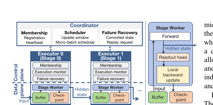
An algorithm that decouples updates is necessary but not sufficient for a fast, robust distributed system — you still have to move tensors between devices, handle stragglers and crashes, and avoid re-introducing synchronization overhead through the back door. Section III of the paper lays out a coordinator/executor architecture (Fig. 2, shown above) and four specific techniques, which the paper is careful to attribute individually to either the throughput or the robustness half of the system’s goals.

(I) Early forwarding. As already highlighted in Algorithm 1’s step 2, the hidden state produced by a chunk’s forward pass is detached and shipped downstream before that chunk’s own local backward pass runs. Why this design and not the obvious alternative? The obvious alternative — forward, then backward, then send — would reintroduce a serialization dependency (downstream waits for upstream’s full local step) even though nothing about local objective construction requires that ordering; early forwarding is a pure win with no correctness cost, because the local backward pass only consumes information already computed during the forward pass (the hidden states $h_{k-1}$ and $h_k$), not anything produced by the backward pass of a downstream chunk. The only place this breaks down, as the paper candidly notes in Section III-C, is the mobile ExecuTorch backend, which by default bundles forward and backward into one atomic method — requiring the custom “pipeline marker operator” workaround described below.

(II) Independent execution and checkpoint. Each executor keeps only its own trainable parameters, optimizer state, and checkpoint. Alternative considered: a global, synchronized checkpoint (as most standard distributed-training checkpointing systems do, ensuring all stages checkpoint at the same logical step) would be simpler to reason about, but would force partial synchronization across stages purely for the sake of checkpoint consistency — defeating the purpose of decoupling in the first place. The cost of the chosen design is a reproducibility subtlety: since each stage checkpoints independently and at its own pace, restoring a training run from checkpoints requires care that all stages’ checkpoints correspond to a consistent-enough point in training, which the failure-recovery mechanism below has to actively manage via replay rather than getting it for free from a shared clock.

(III) State-only inter-stage exchange. Executors ship only the forward hidden state between stages — never gradients, never optimizer state. Where this pays off measurably: Fig. 6(b) (discussed below) shows this is exactly why ZeroLock’s throughput advantage grows as the network link gets slower — baselines that rely on BP must eventually ship a backward gradient tensor of the same size as the forward hidden state across the same link, roughly doubling the communication payload compared to ZeroLock’s forward-only traffic.

(IV) Buffer-assisted state exchange. Each executor keeps a bounded buffer of its upstream stage’s recent hidden states, specifically so it can replay micro-batches after a failure without re-running the upstream computation. Design tension: a larger buffer gives more replay headroom (faster, more localized failure recovery) at the cost of more memory held per stage — the opposite of what the algorithm is otherwise optimizing for. The paper does not report how it tunes this buffer size, which is one of the reproducibility gaps flagged in Section 10 below.

4.1 In-stage execution, spelled out as pseudocode (Algorithm 2)

The paper describes the runtime’s per-micro-batch execution in prose (its “S1/S2/S3” list); unpacking it into an explicit numbered procedure that also shows the inter-stage buffering machinery:

Algorithm 2: ZeroLock Inter-Stage Runtime (coordinator + one executor pair, steady state)
-----------------------------------------------------------------------------------------
State : hidden_state_buffer[k]      // bounded FIFO buffer at executor k, filled by executor k-1
        in_flight_depth_limit        // max unacknowledged entries between a pair of stages
        update_window                // contiguous range of micro-batch indices, set by coordinator
Input : stream of micro-batches indexed 1..M assigned to the current update_window

1:  Coordinator DEFINEs update_window = [i_start, i_end] and micro-batch schedule order
2:  FOR micro-batch i in update_window:
3:      Executor k WAITs on readiness event for hidden_state_buffer[k].entry(i)   // S1: Input
4:          (if k == 1: entry(i) is E(x_i) instead, no wait needed)
5:      Executor k RETRIEVEs h_{k-1,i} from hidden_state_buffer[k], plus mask/position IDs/labels(i)
6:      Executor k EXECUTES Algorithm 1, steps 1-2  (forward + detach + async-send)   // S2
7:      Executor k SUBMITs h_{k,i} into hidden_state_buffer[k+1] via outbound buffer
8:          -- at this point, executor k+1 may immediately begin its own step 3 for micro-batch i --
9:      Executor k EXECUTES Algorithm 1, steps 3-9  (readout, local loss, backprop, accumulate)  // S3
10:     IF i == i_end (last micro-batch in update_window):
11:         Executor k EXECUTES Algorithm 1, steps 11-13  (optimizer step + checkpoint)
12: Coordinator ADVANCEs update_window; PRUNEs hidden_state_buffer entries older than replay horizon
13: ON preposted receive (GPU only): executor k+1 may issue receive_entry(i+1) speculatively
        before executor k finishes producing h_{k,i+1}, overlapping communication setup with compute

Two implementation details matter for correctness and are easy to overlook: the in-flight depth limit (line: in_flight_depth_limit) prevents an unbounded number of unacknowledged hidden-state entries from piling up between a fast upstream stage and a slow downstream one — without it, a fast upstream executor could race arbitrarily far ahead and exhaust the downstream buffer’s memory; and preposted receive (line 13) is a GPU-only optimization that lets the downstream stage register a receive request before the data is ready, so the compute stream only ever waits on the specific readiness event it needs, rather than blocking on unrelated communication traffic.

4.2 Failure recovery: Algorithm 3

Because each stage checkpoints independently and hidden states are buffered rather than immediately discarded, ZeroLock can recover from a single stage’s failure without a full pipeline-wide rollback — a direct structural consequence of technique (II) and (IV) above, not a separate mechanism bolted on afterward.

Algorithm 3: ZeroLock Failure Recovery (triggered when executor k is detected as failed)
------------------------------------------------------------------------------------------
Input : last committed checkpoint for executor k (A_l, B_l, optimizer state, progress metadata)
        hidden_state_buffer[k] contents surviving from before the failure (from upstream, technique IV)
        set of "committed" update windows already fully processed before the failure

1:  Coordinator DETECTs executor k failure (missed heartbeat via membership/execution-monitor)
2:  Coordinator MARKs executor k's in-flight update window(s) as "failed, pending replay"
3:  Executor k RESTORES (A_l, B_l, optimizer state) from its latest local checkpoint     // reactive recovery
4:  Executor k IDENTIFIES the gap: (checkpointed progress) vs. (pipeline frontier reached by other stages)
5:  FOR each micro-batch i in the gap (already buffered upstream, not yet locally re-processed):
6:      Executor k RE-RETRIEVEs h_{k-1,i} from hidden_state_buffer[k]   // no upstream recomputation needed
7:      Executor k RE-EXECUTEs Algorithm 1 (steps 1-13) for micro-batch i     // "replay"
8:  Executor k SIGNALs coordinator once caught up to the pipeline frontier
9:  Coordinator RESUMEs normal scheduling; downstream stages (which stayed alive) never rolled back

Why this design over the obvious alternative (global rollback)? The obvious alternative — used by the paper’s own comparison baseline, synchronous 1F1B — is to roll the entire pipeline back to the last globally-consistent checkpoint and replay from there, because 1F1B’s weight-stashing and shared optimizer step create genuine cross-stage state dependencies that make a purely local rollback incorrect. ZeroLock’s local recovery is only possible because updates never crossed stage boundaries in the first place, so “consistency” was never a global property to begin with — recovering one stage cannot corrupt another stage’s state, because no gradients or shared optimizer state ever flowed between them. Where this could still fail: if the failure occurs during the brief window between a stage completing its local optimizer step and successfully writing its checkpoint, the replay mechanism has to correctly detect that the update was not durably committed and must not double-apply it — the paper does not walk through this edge case explicitly, which is one of the specific gaps noted in the critical-analysis section below.

4.3 The mobile execution backend: a design choice forced by an unexpected constraint

For Android deployment, the paper uses ExecuTorch, Meta’s PyTorch-native on-device runtime, which performs ahead-of-time compilation into a static .pte program for deterministic execution without a Python interpreter. The specific engineering obstacle: ExecuTorch’s training support bundles the forward and backward computation into one atomic method invocation, exposing the forward hidden state only after the local backward gradient computation has already happened — which directly defeats early forwarding (technique I), since by the time you’d have something to send downstream, you have already paid the full local-backward latency you were trying to hide. The fix: the authors insert a custom “pipeline marker” operator into the compiled PTE graph, placed after the detached hidden-state output but before the parameter-gradient subgraph. This operator performs no tensor computation — its only job is to signal the runtime to capture the hidden output and suspend the method’s execution state (stack, tensors, optimizer buffers) at that point. A custom two-phase interface then lets the first phase run up to the marker (returning the hidden state for immediate transfer) and a second phase resume from the suspended state to finish the local backward pass and apply the on-device AdamW update. This is a genuinely clever piece of engineering, precisely because it demonstrates that early forwarding is not merely a scheduling nicety on GPUs but a design property the authors were willing to fight the underlying runtime to preserve on a much more constrained platform — a good signal that the technique matters in practice, not just in the idealized GPU setting.

5. Experiments: does the theory survive contact with a real system?

The paper builds two real prototypes — a multi-GPU/CPU server setup and an Android-phone deployment — and evaluates three things: (E1) memory and throughput versus BP baselines, (E2) failure recovery, and (E3) on-device feasibility. Model and data: TinyLlama, split into three consecutive chunks (one per NVIDIA L40 GPU, or one per Android phone), fine-tuned with LoRA (rank 4, scaling factor 16) on a fixed 10,000-example subset of AG News, sequences padded/truncated to 128 tokens, three random seeds. Baselines: GPipe, 1F1B, and PipeDream (with weight stashing).

5.1 E1: memory and throughput on the GPU prototype

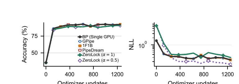
The first and most important sanity check is Fig. 3: does decoupling the chunks actually cost you model quality? The answer is essentially no — ZeroLock’s accuracy curve tracks the BP baselines closely, and its NLL is competitive, with the $\alpha=0.5$ variant (task term and consistency term equally weighted) clearly beating $\alpha=1$ (task term only), which is the empirical confirmation of the intuition discussed in Section 2.2 above: a pure per-chunk task loss without any consistency signal from upstream chunks is a strictly harder learning problem for early, information-poor chunks.

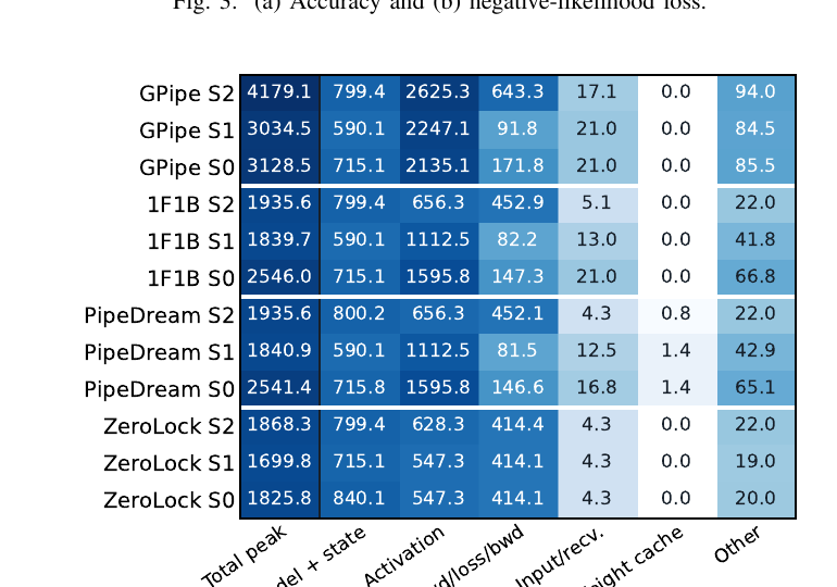
Fig. 4 is the memory story broken down by exactly where the savings come from, and this is the figure I would point to if someone asked “is this actually an activation-memory paper wearing a pipeline-parallelism costume?” The answer is yes, largely: ZeroLock reduces mean per-stage peak memory by 47.8%, 14.7%, and 14.6% versus GPipe, 1F1B, and PipeDream respectively (55.3%, 26.6%, 26.5% for the maximum stage), and the paper explicitly attributes most of this to activation elimination — 75.4%, 40.8%, and 48.8% reduction in the “activation” column specifically. Notice that the “Model + state” and “Weight cache” columns are essentially unchanged across methods (ZeroLock does not touch how LoRA parameters or the base model are stored) — the entire win is concentrated in not having to keep forward activations alive across a chain of pending backward passes, which is exactly the mechanism the paper’s Fig. 1 illustrated conceptually. A secondary but practically important data point buried in the text: GPipe, 1F1B, and PipeDream ran out of memory at physical batch sizes $b = 10, 20, 20$ respectively (with $m=4$), while ZeroLock could scale to $b = 28$ before OOM — meaning the memory savings translate directly into a larger usable batch-size envelope, not just a smaller number on a chart.

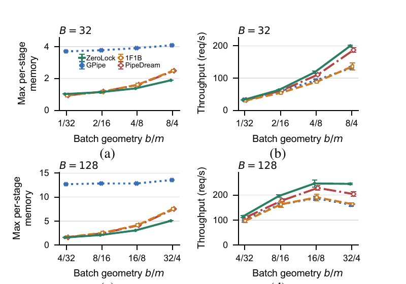
Fig. 5 adds the batch-geometry dimension: as the physical-batch-to-microbatch ratio $b/m$ increases (i.e., fewer, larger microbatch calls before an optimizer step), GPipe’s memory grows sharply because it must hold onto more forward graphs simultaneously, while ZeroLock’s memory grows much more slowly — confirming that the benefit is more pronounced exactly in the regime (large $b/m$) where baseline activation retention is most punishing. On throughput, under the default $b=8, m=4$ setting, ZeroLock improves throughput by 55.8%, 62.8%, and 4.9% over GPipe, 1F1B, and PipeDream respectively — note the much smaller margin over PipeDream specifically, which makes sense given PipeDream is already the most bubble-optimized BP baseline; ZeroLock’s advantage over PipeDream is coming almost entirely from the memory side (enabling larger batches) rather than from eliminating additional scheduling bubbles PipeDream had already mostly eliminated.

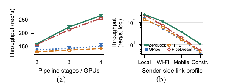
Fig. 6(a) shows ZeroLock’s throughput advantage widening as more stages are added (2 to 4 GPUs) — consistent with removing a dependency that scales with pipeline depth, whereas BP baselines’ bubble overhead compounds with more stages. Fig. 6(b) is the figure that most directly validates design choice (III) from Section 4: as the simulated network link gets slower (Local -> Wi-Fi -> Mobile -> Constrained, with bandwidths dropping from about 1000 Mbps to 50 Mbps and latency rising from about 0 to 30 ms), ZeroLock’s relative throughput advantage over 1F1B and PipeDream grows, precisely because those baselines must ship a backward gradient tensor across the same link in addition to the forward hidden state, while ZeroLock only ever ships the forward hidden state.

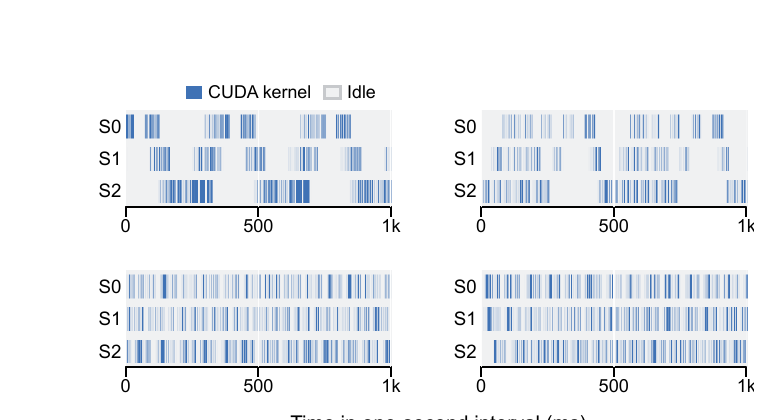
Fig. 7 is a nice piece of mechanistic evidence rather than a summary statistic: you can visually see GPipe’s stages (a) have long, block-structured idle gaps (the classic “fill-then-drain” bubble pattern), 1F1B (b) has shorter but still-visible gaps, and PipeDream (c) and ZeroLock (d) both look far denser — but the paper reports ZeroLock achieves a more balanced activity load across stages than PipeDream specifically, with a 13.7% higher active fraction, which the text is careful to caveat is “a diagnostic indicator of pipeline scheduling rather than a proxy for throughput,” since idle time also includes host dispatch and Gloo communication overhead unrelated to the algorithm itself. I appreciated this caveat — it is exactly the kind of honesty about what a metric does and does not measure that I want more systems papers to include.

5.2 E2: failure recovery

Using three stages with $b=1, m=8$, the paper injects a failure at Stage 1 during a mid-training window (four “prelude” windows, then four “failure” windows at Stage 1, then four “resumed” windows), keeping worker processes and GPU contexts alive throughout (a fault-injection design that isolates the recovery protocol’s cost from raw process-restart cost). Compared with synchronous 1F1B’s global-rollback-and-full-replay recovery, ZeroLock’s local recovery reduces recovery latency by 368 ms (2013.1 ± 6.4 ms vs. 2381.2 ± 66.6 ms) and cuts transfer traffic in half (96 MiB vs. 192 MiB) — both numbers directly reflecting that only the failed stage needs to replay, rather than the whole pipeline needing a synchronized rollback.

5.3 E3: on-device evaluation with Android phones

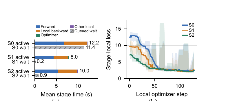
The paper deploys three TinyLlama training PTEs (covering transformer layers [0,6], [7,13], [14,21]) across an NX809J, a Lenovo L71091, and a Pixel 10 Pro XL, training on 128 samples at sequence length 128 with LoRA rank 8. The headline numbers: peak PSS under 4000 MiB, battery temperature around 37°C, and a full fine-tuning wall-clock time of 1644.1 s (throughput 0.0779 records/s) — modest by server standards, but the point is feasibility, not speed: this is, to my knowledge, one of the first BP-free local-objective pipeline training demonstrations running end-to-end on unmodified consumer Android hardware. Fig. 8(a) shows each device’s active-vs-wait time is fairly balanced (S0 waits 11.4s against 12.2s active, roughly matching S1 and S2’s ratios), suggesting the three heterogeneous devices are reasonably load-balanced despite having quite different compute capabilities, though the paper does not explain whether this balance was achieved by design (e.g., uneven layer-count partitioning to compensate for device heterogeneity) or is coincidental to this particular hardware trio. Fig. 8(b) shows all three stages’ local losses converging over about 125 optimizer steps, with S0 (the earliest, most information-poor chunk) starting from and settling at a visibly higher loss than S2 — a nice empirical echo of the $\alpha=1$ discussion in Section 2.2: even with the consistency term active, earlier chunks structurally face a harder local prediction problem than later ones.

6. Design choices, revisited: why this and not the obvious alternative

Beyond the four system techniques already discussed in Section 4, three algorithmic design choices deserve explicit why/alternative/boundary treatment, since they are easy to gloss over on a first read.

Frozen, shared readout head vs. per-chunk trainable heads. ZeroLock reuses the pretrained model’s own final normalization layer and LM head as the readout for every intermediate chunk (the “(a) Static Model Head” option in Section III-B), rather than training a separate small classifier head per chunk (which is what several prior local-learning methods for vision models do). The alternative — per-chunk trainable heads — would add trainable parameters and require the intermediate representation to be interpreted by a head specifically trained for that depth, whereas the frozen shared head lets every chunk’s local loss be directly comparable in scale and directly informative about “how close is this intermediate representation to something the final layer could already read.” Where this breaks down: the paper itself flags that this assumes intermediate hidden states are “interpretable” by the final head, which the authors admit “may not hold for complex generative tasks” — this is precisely why they also provide the readout-adapter option (b), a small residual MLP initialized near identity, as a fallback for cases where the raw intermediate representation and the frozen head’s expected input space diverge too much. Notably, none of the experiments in Section IV actually use option (b) or report when it becomes necessary, leaving open exactly how far the “readable by the final head” assumption can be stretched before quality degrades.

KL/Bregman divergence for the consistency term vs. a simpler L2 or feature-matching loss. Enforcing consistency at the level of the predictive distribution $p_{k-1}$ (i.e., matching what the previous chunk would have predicted as the next token) rather than at the level of the raw hidden state $h_{k-1}$ (i.e., an L2 or cosine loss between hidden vectors) is what makes Lemma 1 and the entire convergence machinery in Section 3 work — the whole proof pipeline depends on being able to write both the task loss and the consistency loss as Bregman divergences over the same probability-simplex space $\mathcal{P}$, so that the local optimum (Eq. 7) can be expressed in terms of the global objective’s gradient. A hidden-state-space consistency loss would sidestep needing a readout head at every chunk at all, and might be cheaper to compute, but would not admit the same clean reduction to a proximal-gradient step on a scalar objective, because Euclidean or cosine similarity in hidden-state space has no obvious relationship to the KL-divergence-based global cross-entropy objective the model is ultimately trained on. This is a case where the theoretically convenient choice and the practically motivated choice happen to coincide, which is worth calling out as a genuinely good piece of design, not just a lucky accident — the readout head is doing double duty as both “how you compute a local loss at all” and “the object that makes the theory tractable.”

Fixed, per-run scalar $\alpha$ vs. a learned or per-token-adaptive blend weight. The blend weight $\alpha$ in Eq. (3) is treated as a single global hyperparameter, tuned once per run (the paper compares only $\alpha=1$ and $\alpha=0.5$ in Fig. 3). An adaptive alternative — e.g., increasing $\alpha$ for later chunks (which have seen more context and might reasonably weight the task term more heavily) or decreasing it early in training (when the consistency target $p_{k-1}$ is itself still noisy) — seems like a natural refinement given the paper’s own finding that $\alpha=0.5$ clearly beats $\alpha=1$. The paper does not explore this design space at all, which is a missed opportunity: Proposition 1’s error bound explicitly depends on $\alpha$ through the $(1/\alpha - \beta)$ contraction term and the $\delta_k/\alpha$ error term, so there is a theoretically motivated reason to expect a per-chunk-tuned or per-iteration-scheduled $\alpha$ could improve on a single global constant, but this remains unexplored in the current paper.

7. Limitations the paper is upfront about, and a few it is not

The paper is reasonably candid about several of its own boundaries: (a) the static-model-head design assumes intermediate hidden states are interpretable by the final head, which may not hold for complex generative tasks; (b) the theoretical framework in Section II-C relies on standard non-convex SGD assumptions (bounded gradient, smoothness, Lipschitz continuity, bounded-variance sampling) that, while common in the literature, are genuinely strong assumptions for a deep transformer’s loss landscape and are not independently verified for the specific TinyLlama + LoRA setting used in the experiments; (c) the paper’s own future-work note says it would be “meaningful to further incorporate operator-level optimization to further improve throughput and reduce memory usage” — an implicit admission that the current system-level implementation is not yet operator-optimized, so the reported throughput numbers likely understate what a more mature implementation could achieve (in either direction, since baselines are equally un-optimized at the operator level, but it does mean the reported percentages are specific to this implementation’s maturity, not necessarily to the algorithm’s ceiling).

Several limitations the paper does not fully surface, in my reading:

• Scale. Every experiment uses TinyLlama (a ~1.1B-parameter model) split into only three chunks. Nothing in the paper’s theory forbids scaling to larger models or more chunks, and Proposition 1’s error-accumulation bound is explicitly framed for general $K$, but there is zero empirical evidence for how $\delta_k$ (the per-chunk suboptimality gap that drives the accumulated-error term) behaves as chunk count grows past 3 or as the base model grows past 1B parameters — precisely the regime where pipeline parallelism actually matters in practice (nobody pipeline-parallelizes a 1.1B model across three L40s for a production reason; you do it to prototype).
• Task diversity. The one fine-tuning task evaluated (AG News, a short-sequence text classification-flavored dataset at 128 tokens) is a relatively easy setting for the “interpretable-by-final-head” assumption to hold, since news-topic signal is likely present quite early in a forward pass. It would be informative — and is a natural next experiment — to see how the accuracy gap between ZeroLock and BP behaves on tasks requiring long-range reasoning across the full sequence (e.g., long-document QA or multi-step arithmetic), where an early chunk’s local prediction is plausibly a much worse proxy for the eventual correct answer.
• The readout-adapter fallback is unevaluated. Since option (b) exists specifically as a hedge against the interpretability assumption failing, and the paper does not report a single experiment using it, we have no empirical sense of when a practitioner should reach for it, or how much overhead/quality change it introduces relative to the default static head.
• No compute/wall-clock accounting for the extra readout-head forward passes. Attaching a readout head after every chunk (not just the last) means $K$ separate softmax-and-cross-entropy computations per micro-batch instead of one — for a vocabulary size in the tens of thousands, this is not free, and the paper’s memory breakdown (Fig. 4) and throughput numbers presumably already include this cost implicitly, but the paper never isolates or quantifies it as its own line item, making it hard to know how this overhead would scale with vocabulary size or with $K$.

8. Critical analysis: what I would push back on

(a) Weaknesses and flaws specific to this paper. The single biggest gap is the mismatch in scale between the theoretical framing (general $K$, general model architecture, general chunk division) and the empirical validation (one 1.1B model, three chunks, one short-sequence classification-style task). Theorem 1’s convergence rate is asymptotic in $T$ and does not depend on $K$ in its stated form, which is a clean and appealing result, but the constants hidden inside $\tilde{\mathcal{O}}$ (specifically $\beta_R(\alpha)$, $\sigma(\alpha)$, and $D_T(\alpha)$) could plausibly grow with $K$ in ways the paper does not analyze, and the empirical results give no signal either way because $K=3$ is never varied. A reader coming away from this paper might reasonably (over-)generalize “ZeroLock scales to arbitrary pipeline depth with the same theoretical guarantees,” when the honest claim the evidence supports is closer to “ZeroLock’s theory holds for general $K$ in the abstract, and works well in practice for $K=3$.”

(b) Limitations the authors understate or omit. The comparison table in Fig. 4/5/6 is exclusively against BP-based pipeline baselines (GPipe, 1F1B, PipeDream); the paper’s own related-work section (footnote 5) explicitly notes that comparing against the other BP-free local-objective baselines (PPLL, FluidPipe, SCPL, LoPT) was not done because those works either lack open-source code, are not designed for LLM fine-tuning, or do not implement genuine multi-GPU system-level pipeline parallelism. This is a defensible practical reason, but it also means the paper never empirically demonstrates that ZeroLock’s specific local-objective design (task term + consistency term via a shared frozen readout head) is better than the alternative local-objective designs it explicitly critiques in the related-work discussion (e.g., SCPL’s per-segment supervised contrastive loss, or LoPT’s two-chunk-restricted approach) — the critique of those methods is conceptual/qualitative, not experimental. Additionally, the failure-recovery experiment (E2) injects exactly one failure at one stage in a controlled, contrived window; there is no evaluation of concurrent multi-stage failures, or of failures that occur mid-checkpoint-write (the specific edge case flagged in Section 4.2 above).

(c) Concrete, specific improvement suggestions. First, run the same memory/throughput/failure-recovery suite at $K \in \{4, 8, 16\}$ chunks on a model in the 7B-13B range, to actually test whether the “general chunk division” theoretical framing pays off at the model sizes where pipeline parallelism is normally deployed for real reasons rather than as a research prototype convenience. Second, report $\delta_k$ (the local-optimum suboptimality from Proposition 1) empirically across chunks and training steps — this is directly measurable (it is just $D_\psi(p_k, p_k^\star)$, and $p_k^\star$ can be approximated numerically for a held-out validation batch) and would let readers see whether the error-accumulation term the theory warns about is in practice negligible or a real constraint on how many chunks you can use. Third, add at least one long-range-dependency task (e.g., needle-in-a-haystack retrieval or multi-hop QA at 4K+ tokens) to stress-test the interpretable-by-final-head assumption underlying the static readout head, since AG News at 128 tokens is close to a best-case scenario for that assumption. Fourth, directly benchmark against at least one of the BP-free local-objective competitors mentioned in footnote 5 (even a task-restricted, single-node reproduction of SCPL or LoPT’s core update rule, without full system-level pipeline parallelism) so that the accuracy/throughput comparison in Fig. 3-6 isn’t exclusively against a different algorithmic family (BP) but also against the closest conceptual competitors.

9. Reproducibility notes

The paper provides a code link (https://anonymous.4open.science/r/unlock_trainer-105B, an anonymized submission repository), which is a positive signal, though I was not able to independently verify its contents as part of this review. Reported hyperparameters are reasonably complete for the GPU experiments (LoRA rank 4, scaling 16, three chunks/L40 GPUs, AG News subset of 10,000 examples, sequence length 128, three random seeds) and for the mobile experiments (LoRA rank 8, scaling 16, learning rate $10^{-4}$, 128 samples, sequence length 128, $b=1$). Missing or under-specified details that would matter for a from-scratch reproduction: the exact learning-rate schedule and optimizer (AdamW is mentioned only for the mobile backend, not explicitly confirmed for the GPU experiments); the specific values of $\eta_0$ and $\gamma$ used in the theoretical step-size schedule $\eta_t = \eta_0/\sqrt{t+\gamma}$ versus whatever practical schedule was actually used in the experiments (these need not be the same, but the paper does not clarify); the in-flight-depth-limit and hidden-state-buffer-size values used for the runtime; and the precise chunk boundaries (which layers went into which of the three chunks) beyond the Android deployment’s [0,6]/[7,13]/[14,21] split, which is not confirmed to match the GPU experiments’ partitioning. The paper’s “Use of AI Disclosure” section is a nice piece of transparency that more systems papers should include, explicitly noting ChatGPT was used for environment setup, benchmark migration, Kotlin code generation for mobile deployment, and batch experiment scripting, with the authors taking responsibility for final validation.

10. Conclusion

ZeroLock is a rare paper that pairs a genuinely new theoretical result (the first convergence analysis for local-objective-construction-based BP-free training under general chunk division, matching BP’s $\mathcal{O}(1/\sqrt{T})$ rate up to a polylog factor) with a real, working, cross-platform system (multi-GPU server and unmodified Android phones) and honest, mechanistically-grounded experiments that show where the gains come from rather than just that they exist. The core idea — decouple pipeline stages by giving each one its own local objective built from a shared frozen readout head, rather than trying to schedule around backpropagation’s chain-rule dependency — is conceptually clean and, per the theory, essentially free asymptotically. What keeps this from being an unqualified triumph is the gap between the generality of the theory and the narrowness of the empirical validation: three chunks, one 1.1B model, one short-sequence classification-flavored task. If the follow-up work stress-tests exactly the axes this paper leaves open — more chunks, bigger models, longer-range tasks, and a head-to-head comparison against the other BP-free local-objective methods it currently only discusses qualitatively — ZeroLock’s core idea looks like it has real staying power as a genuine alternative lever (alongside, not instead of, scheduling-based bubble reduction) for memory- and communication-constrained pipeline training.