CVPO: Curriculum-Guided Value-Variance Policy Optimization for LLM Reasoning

Review date: 2026-08-11 Author: Zhongzhu Zhou Paper reviewed: CVPO: Enhancing LLM Reinforcement Learning Reasoning via Value-Variance Adaptation and Dynamic Curriculum Learning Paper authors: Ziqi Jia, Yalu Ouyang, Bo Pang, Panpan Li, Hangfei Xu, Shengzhao Wen, Shiyong Li, Yanpeng Wang (Baidu AI Cloud Group, Tsinghua University, UC San Diego) arXiv: 2608.03068 Venue/Status: Preprint (cs.CL), August 2026

1. Why a value-based RL method still needs more signal

If you’ve been following the RLHF-for-reasoning literature, you’ve likely absorbed a simple story: GRPO (used by DeepSeek-R1 and friends) dropped the value network entirely and normalized rewards within a group of sampled trajectories to get an advantage estimate — cheap, stable, and surprisingly effective. Then VAPO and VC-PPO pushed back: a well-trained value model, if you fix the classic PPO failure modes (value initialization bias, reward decay over long chains-of-thought, GAE bias-variance mismatch at long horizons), gives you a strictly more accurate credit-assignment signal than GRPO’s coarse group-average, and empirically outperforms it.

CVPO’s starting observation is that even a well-trained value model is being under-used. A value model doesn’t just give you a point estimate $V(s)$ at each token — if you actually look at how that value estimate fluctuates across the tokens of a single generated trajectory, you get a second, entirely separate signal: how much internal uncertainty/exploration happened while producing this particular response. Two trajectories can receive the identical scalar reward (+1 for a correct final answer) while having wildly different token-level value trajectories — one confidently marching toward the boxed answer, the other bouncing around uncertainly before stumbling onto the right result. Existing value-based advantage functions (plain GAE-based advantages, as in PPO/VAPO) treat both of these trajectories identically once the terminal reward is fixed. CVPO’s core methodological move is to not treat them identically: it uses the variance of the trajectory’s token-level value sequence as a second-order signal that modulates the size of the advantage, differently for correct and incorrect trajectories.

Layered on top of this trajectory-level mechanism is a second, orthogonal problem: difficulty drift. As an RL-trained policy improves over thousands of steps, questions that were “hard” (near-zero accuracy) early in training gradually become “medium” or “easy.” A curriculum that was well-calibrated to problem difficulty at step 0 is stale by step 1500. CVPO addresses this with a Bayesian tracker of per-question accuracy and a hand-designed reweighting function that shifts attention from “medium-difficulty” problems (useful early, because they carry the most learning signal per sample) toward “hard, currently-unsolved” problems once the easy ones are mastered — while explicitly zeroing out the weight of fully-solved questions to avoid wasted compute.

The net method, CVPO, multiplies these two independently-motivated correction terms into the advantage used by an otherwise-standard PPO-style value-based training loop, and reports substantial gains over VAPO and a hand-tuned single-step asynchronous variant of GRPO on AIME24/25, AMC23/24, and MATH-500 with a Qwen2.5-7B base model.

It’s worth situating this against the broader curriculum-learning-for-RL literature the paper cites (Qu et al.’s online difficulty prediction, Parashar et al.’s easy-to-hard curricula, Shi et al.’s adaptive curriculum reinforcement finetuning): most prior curriculum approaches for LLM RL define difficulty either as a static, pre-computed property of the dataset (e.g., human-annotated difficulty tags, or a separate model’s pass-rate estimate computed once before training starts) or as a coarse global schedule (train on progressively harder buckets in a fixed order). CVPO’s Bayesian per-question tracker is explicitly online and policy-relative — difficulty is redefined continuously as “how well does the current policy do on this question,” which is the more principled framing given that difficulty drift is fundamentally about the policy’s own capability changing, not about any fixed property of the question itself. This distinction matters in practice: a static curriculum computed against a weaker reference model will misjudge which questions are “medium difficulty” for the policy actually being trained, especially many steps into training.

Prerequisites: what you need before the method makes sense

RL for LLM reasoning as a token-level MDP. Treat text generation as a sequential decision process: the “state” $s_t = (x_0, \ldots, x_m, y_0, \ldots, y_t)$ is the prompt plus everything generated so far, the “action” $a$ is the next token drawn from a fixed vocabulary, and the transition is deterministic (appending the chosen token). A trained policy $\pi_\theta$ (the LLM itself) assigns a probability to each possible next token given the state; training adjusts $\theta$ to make the policy more likely to produce trajectories that earn higher reward. In math-reasoning RL, reward is usually terminal and sparse: +1 if the final boxed answer matches ground truth, −1 (or 0) otherwise — there’s no intermediate per-token reward telling you “this step of the derivation is good.”

PPO and the advantage function. Vanilla policy gradient says: increase the log-probability of actions that led to more reward than expected, decrease it for actions that led to less. The “more than expected” part is formalized as the advantage $A(s,a) = Q(s,a) - V(s)$: how much better was taking action $a$ in state $s$ compared to the average action the policy would have taken there. PPO uses a clipped surrogate objective (Eq. 1 below) so that a single update step can’t move the policy too far from where it was, and estimates the advantage using Generalized Advantage Estimation (GAE, Eq. 2), a weighted sum of one-step TD residuals $\delta_t = r_t + \gamma V(s_{t+1}) - V(s_t)$ that trades off bias and variance via a parameter $\lambda$.

$$L(\theta) = \mathbb{E}_t\Big[\min\big(r_t(\theta)\hat{A}_t,\ \mathrm{clip}(r_t(\theta), 1-\epsilon, 1+\epsilon)\hat{A}_t\big)\Big] \tag{1}$$ $$\hat{A}_t = \sum_{k=0}^{T-t-1} (\gamma\lambda)^k \delta_{t+k}, \qquad \delta_t = r_t + \gamma V(s_{t+1}) - V(s_t) \tag{2}$$

Here $r_t(\theta) = \frac{\pi_\theta(a_t \mid s_t)}{\pi_{\theta_{\text{old}}}(a_t \mid s_t)}$ is the importance-sampling ratio between the new and old policy, $\epsilon$ bounds how far that ratio is allowed to move in one update, $\gamma$ is the discount factor, and $V(s)$ is a learned value function (a small head, usually attached to the same or a similarly-sized transformer, trained to regress the empirical return).

GRPO: throwing away the value model. GRPO (used in DeepSeek-Math and DeepSeek-R1) sidesteps the need to train a value model at all: sample a group of $G$ trajectories for the same prompt, compute each trajectory’s scalar terminal reward, then normalize within the group — $A_i = \frac{r_i - \text{mean}(r_{1:G})}{\text{std}(r_{1:G})}$ — and use this group-relative score as every token’s advantage in that trajectory. This is cheap (no value network to train) and stable, but coarse: every token in a trajectory gets the same advantage regardless of how that token individually contributed, and if all $G$ sampled trajectories for a prompt happen to be correct (or all incorrect), the group has zero variance and produces no learning signal at all — a homogeneity failure mode that motivates value-based methods.

VAPO/VC-PPO: making value-based PPO work for long chains-of-thought. The naive combination of PPO + a value network trained from scratch is known to be unstable for long reasoning chains: the value network is poorly calibrated early in training (initialization bias) and its bootstrapped targets in Eq. 2 propagate errors across very long trajectories (reward signal decay). VC-PPO fixes this with a value-model pretraining phase and decoupled GAE parameters for the value update vs. the policy update. VAPO adds length-adaptive GAE (the $\lambda$ used in Eq. 2 is adjusted based on trajectory length, since longer chains need different bias-variance trade-offs) and token-level rather than sequence-level losses. CVPO explicitly builds on top of a VAPO-style value-based pipeline — it inherits VAPO’s decoupled GAE and length-adaptation, and adds the two mechanisms described below.

2. Mechanism 1 — why value-variance bounds the policy gradient (the theory)

The paper’s first contribution is a short, clean derivation showing that the variance of the advantage function directly bounds the magnitude of the policy gradient. This is worth walking through in full, because it’s the theoretical justification for treating variance as a first-class training signal rather than noise to be averaged away.

Start from the standard policy gradient (the quantity every RL update tries to estimate):

$$\nabla_\theta J(\theta) = \mathbb{E}_{s,a\sim\pi_\theta}\big[\nabla_\theta \log \pi_\theta(a\mid s)\cdot A(s,a)\big] \tag{3}$$

where $A(s,a) = Q(s,a) - V(s)$ as before. Assume the gradient of the log-policy is bounded in $L_2$ norm by some constant $C$ (a standard regularity assumption — in practice this is roughly enforced by the clipping in Eq. 1 and by gradient clipping during optimization):

$$\lVert \nabla_\theta \log\pi_\theta(a\mid s) \rVert_2 \le C. \tag{4}$$

Step 1 — Cauchy–Schwarz to separate the two factors. The gradient in Eq. 3 is an expectation of a product of two random quantities (the score-function gradient and the advantage). Applying Cauchy–Schwarz inside the expectation (bounding the norm of a product by the product of norms) and then substituting the assumption in Eq. 4:

$$\lVert \nabla_\theta J(\theta) \rVert_2 \le \mathbb{E}\big[\lVert \nabla_\theta \log\pi_\theta(a\mid s)\rVert_2 \cdot |A(s,a)|\big] \le C\cdot \mathbb{E}[|A(s,a)|]. \tag{5}$$

This says: the gradient norm is controlled by how large the advantage typically is, in absolute value — intuitively, the more “surprising” an action’s payoff, the larger the parameter update it induces.

Step 2 — relate $\mathbb{E}[|A|]$ to $\mathrm{Var}(A)$. We can’t directly compute $\mathbb{E}[|A|]$ from the moments PPO already estimates, but we can bound it using the variance of $A$, which is a quantity we can estimate from the value model’s outputs. Since the advantage is, by construction, mean-zero under the policy that generated it ($\mathbb{E}[A(s,a)] = 0$ — this is the entire point of subtracting a baseline), its variance simplifies to a second moment:

$$\mathrm{Var}(A) = \mathbb{E}[A(s,a)^2]. \tag{6}$$

Jensen’s inequality applied to the convex function $x \mapsto x^2$ gives $(\mathbb{E}[|A|])^2 \le \mathbb{E}[A^2]$, i.e.

$$(\mathbb{E}[|A(s,a)|])^2 \le \mathbb{E}[A(s,a)^2] = \mathrm{Var}(A) \implies \mathbb{E}[|A(s,a)|] \le \sqrt{\mathrm{Var}(A)}. \tag{7-8}$$

Step 3 — expand $\mathrm{Var}(A)$ in terms of $Q$ and $V$. Since $A = Q - V$, elementary variance algebra gives

$$\mathrm{Var}(A) = \mathrm{Var}(Q) + \mathrm{Var}(V) - 2\,\mathrm{Cov}(Q, V). \tag{9}$$

To turn this into an upper bound (we want a worst-case statement, so we need to eliminate the covariance term, whose sign we don’t know a priori), apply the Cauchy–Schwarz inequality for covariances, $|\mathrm{Cov}(Q,V)| \le \sqrt{\mathrm{Var}(Q)\mathrm{Var}(V)}$, and take the worst case where the covariance is maximally negative (which maximizes $\mathrm{Var}(A)$):

$$\mathrm{Var}(A) \le \mathrm{Var}(Q) + \mathrm{Var}(V) + 2\sqrt{\mathrm{Var}(Q)\mathrm{Var}(V)} = \big(\sigma_Q + \sqrt{\mathrm{Var}(V)}\big)^2, \qquad \sigma_Q := \sqrt{\mathrm{Var}(Q)}. \tag{10-11}$$

This is just recognizing $(a+b)^2 = a^2 + b^2 + 2ab$ with $a = \sigma_Q$, $b=\sqrt{\mathrm{Var}(V)}$ — the algebra is elementary, but the payoff is that we now have a bound purely in terms of the two individual variances, no cross term.

Step 4 — chain everything together. Substituting Eq. 11 into Eq. 8, then Eq. 8 into Eq. 5:

$$\mathbb{E}[|A(s,a)|] \le \sigma_Q + \sqrt{\mathrm{Var}(V)} \tag{12}$$ $$\lVert \nabla_\theta J(\theta) \rVert_2 \le C\cdot\Big(\sigma_Q + \sqrt{\mathrm{Var}(V)}\Big). \tag{13}$$

What this buys you. Eq. 13 is a genuine, if loose, theoretical statement: the magnitude of the policy update is controlled by the variance of the value estimate $\mathrm{Var}(V)$ (plus a term from the intrinsic randomness of the environment/reward, $\sigma_Q$, which the training algorithm cannot directly manipulate). If you can measure $\mathrm{Var}(V)$ at the trajectory level, and you deliberately push it up for trajectories where you want more exploration (bigger updates) and down for trajectories where you want convergence (smaller updates), you are directly manipulating the achievable gradient magnitude according to Eq. 13 — this is the theoretical license for the design in Section 3. It’s worth being honest about what the theorem does not say: it’s an upper bound, not an equality, so a high $\mathrm{Var}(V)$ permits large gradients but doesn’t guarantee them, and the bound doesn’t say anything about the direction of the gradient, only its magnitude. The paper is explicit that this is a “principled” motivation rather than a tight guarantee — a distinction that matters when judging how much weight to put on the theory versus the empirical ablations later.

3. Mechanism 1 in practice — the stochasticity-aware advantage correction

The theory says “modulate $\mathrm{Var}(V)$ deliberately.” The practical question is: modulate it how, and in which direction for which trajectories? CVPO’s answer rests on an empirical observation illustrated by the paper’s Figure 1 — a word cloud of the tokens that receive the highest average value estimates from the trained value model.

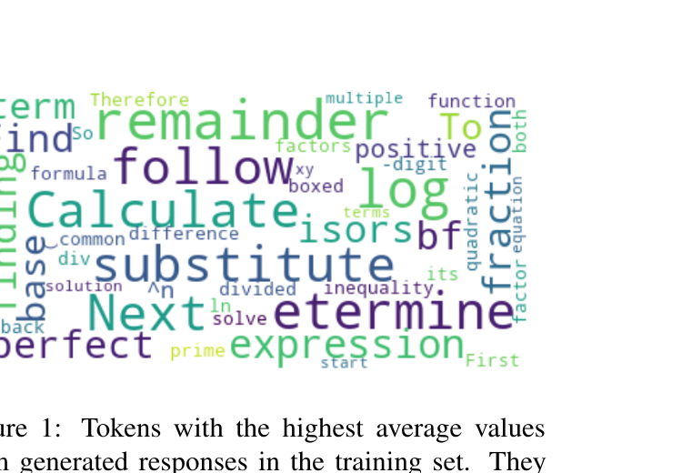
The intuition: tokens central to the actual reasoning process (operators, key mathematical terms, transition words like “Therefore”/“Next”) receive systematically different value estimates than filler tokens. If you track how the value estimate changes token-to-token across a single generated response — i.e., its variance along the trajectory — you get a proxy for how much genuine exploration/deliberation happened while producing that response, as opposed to a rote, low-variation continuation. High intra-trajectory value variance = the model was actively “considering” different directions; low variance = a rigid, low-exploration response.

Design choice — why variance-of-value rather than variance-of-reward or entropy-of-action-distribution? The obvious alternatives are (a) the policy’s token-level entropy, which is already tracked in most RL pipelines as an exploration proxy, or (b) reward variance across a rollout group (essentially what GRPO already normalizes by). The paper doesn’t use either. Entropy measures uncertainty in the action distribution at a single step, which is noisy and doesn’t distinguish “genuinely deliberating about a hard sub-problem” from “the token itself is inherently ambiguous” (e.g., choosing between two synonyms). Value variance, by contrast, is a value-model-mediated signal that has already been trained to track long-horizon consequences of a state, not just the next-token distribution — so a spike in value variance is closer to “this state is a fork in the road that matters for the final answer” than a spike in entropy would be. The boundary condition the paper doesn’t discuss: this argument only holds if the value model itself is well-calibrated (recall VAPO’s whole point was that value models are not well-calibrated by default) — a poorly-calibrated value model would produce a value-variance signal that’s really just noise dressed up as a meaningful exploration proxy.

3.1 The mechanism, unpacked step by step

Given a batch of $B$ sampled trajectories $\mathcal{B} = \{(v_i, r_i, \mathrm{idx}_i)\}_{i=1}^{B}$, where $v_i \in \mathbb{R}^{T_i}$ is the sequence of per-token value estimates for trajectory $i$ and $\mathrm{idx}_i$ identifies which prompt it came from (recall that multiple trajectories are sampled per prompt, exactly as in GRPO’s group sampling):

Step 1 — per-trajectory variance signal. Compute the standard deviation of the value sequence within each trajectory:

$$\sigma_i = \mathrm{std}(v_i). \tag{sig-i}$$

Step 2 — group-relative normalization. A raw $\sigma_i$ isn’t directly comparable across prompts of very different inherent difficulty (a hard problem might legitimately induce higher value variance throughout, regardless of exploration quality). So the paper normalizes each trajectory’s variance against the other trajectories sampled for the same prompt — let $\mathcal{G}_k = \{i \mid \mathrm{idx}_i = k\}$ be the trajectories sampled for prompt $k$:

$$\mu_k = \frac{1}{|\mathcal{G}_k|}\sum_{i \in \mathcal{G}_k} \sigma_i. \tag{14}$$

$\mu_k$ is now a same-prompt reference point: “is this particular trajectory’s exploration level unusually high or low, compared to its siblings sampled for the same question?” This is analogous to how GRPO normalizes reward within a group rather than across the whole batch — same design pattern, applied to a different statistic.

Step 3 — asymmetric weighting by trajectory outcome. This is the crux of the mechanism, and it directly encodes the paper’s central heuristic: correct trajectories should converge (penalize high variance = punish “lucky, meandering” correct answers), incorrect trajectories should keep exploring (penalize low variance = punish “rigidly wrong” answers).

For correct trajectories ($R(\tau)=1$):

$$W_S(\mathrm{Var}(\tau), 1) = 1.0 + \alpha_P \cdot \mathrm{sigmoid}\big(\lambda_P(\mathrm{Var}(\tau) - \mu_k)\big). \tag{15}$$

For incorrect trajectories ($R(\tau)=0$):

$$W_S(\mathrm{Var}(\tau), 0) = 1.0 - \alpha_N \cdot \mathrm{sigmoid}\big(\lambda_N(\mu_k - \mathrm{Var}(\tau))\big). \tag{16}$$

Reading Eq. 15: if a correct trajectory’s variance exceeds its group’s mean ($\mathrm{Var}(\tau) - \mu_k > 0$), the sigmoid saturates toward 1 and the weight grows toward $1+\alpha_P$ — a penalty multiplier, since in CVPO’s actual advantage sign convention (Section 3.3) larger $W_S$ on a correct trajectory means the model is pushed harder toward a low-variance, “locked-in” policy at that state, discouraging further meandering once a correct path is found. If the variance is below the group mean, the sigmoid goes toward 0 and $W_S \to 1.0$ — no penalty, the “efficient, confident, correct” trajectory is left alone.

Reading Eq. 16: if an incorrect trajectory’s variance is below its group mean ($\mu_k - \mathrm{Var}(\tau) > 0$, i.e., this wrong answer was produced rigidly, without much internal deliberation), the sigmoid saturates and $W_S \to 1 - \alpha_N$ — a reduced-magnitude penalty, i.e., go easier on the model for being wrong here, because the actual problem was insufficient exploration, and further punishing a low-exploration failure just reinforces the rigidity. If the variance is above the group mean (this wrong answer at least involved active exploration, just landed on the wrong result), $W_S \to 1.0$ — full penalty strength, because exploration alone doesn’t excuse an incorrect final answer.

Design choice — why sigmoid gating rather than a hard threshold? A hard threshold ($W_S = 1+\alpha_P$ if $\mathrm{Var}>\mu_k$ else $1.0$) would create a training-destabilizing discontinuity exactly at trajectories near the group mean — small stochastic fluctuations in $\mathrm{Var}(\tau)$ estimation (itself a noisy quantity, computed from a single rollout’s value sequence) would flip the weight abruptly. The sigmoid gives a smooth interpolation, at the cost of two extra hyperparameters ($\lambda_P, \lambda_N$ controlling steepness) that must be tuned. The paper doesn’t report a sensitivity study for these steepness parameters specifically (it does for the overall variance coefficient, discussed below), which is a gap in the ablation coverage.

Step 4 — numbered algorithm. Putting the four steps together as pseudocode:

Algorithm 1: Stochasticity-Aware Advantage Correction
Input: batch of trajectories B = {(v_i, r_i, idx_i)}_{i=1..B}, params alpha_P, alpha_N, lambda_P, lambda_N
Output: per-trajectory weight W_S,i for each trajectory i

1:  for each trajectory i in B:
2:      sigma_i <- std(v_i)                      # Eq. (sig-i): intra-trajectory value variance
3:  for each prompt k (grouping trajectories by idx_i):
4:      G_k <- { i : idx_i = k }
5:      mu_k <- mean( sigma_i for i in G_k )       # Eq. (14): group-relative reference variance
6:  for each trajectory i in B:
7:      k <- idx_i
8:      if r_i == 1 (correct trajectory):
9:          W_S,i <- 1.0 + alpha_P * sigmoid( lambda_P * (sigma_i - mu_k) )    # Eq. (15)
10:     else (incorrect trajectory):
11:         W_S,i <- 1.0 - alpha_N * sigmoid( lambda_N * (mu_k - sigma_i) )    # Eq. (16)
12: return { W_S,i }

This algorithm runs once per training batch, after rollout generation and value-model scoring but before the advantage is finally assembled — it’s a cheap post-processing step over already-computed value estimates, not an additional forward/backward pass, which is an important practical property: the mechanism adds essentially zero extra compute to the training loop.

3.2 A worked numerical example

It helps to trace concrete numbers through Eq. 15-16 rather than reason about them purely symbolically. Suppose a prompt $k$ has 4 sampled trajectories with value-sequence standard deviations $\sigma = [0.008,\ 0.015,\ 0.006,\ 0.020]$, correctness labels $R = [1,\ 1,\ 0,\ 0]$, and suppose the tuned hyperparameters are $\alpha_P = \alpha_N = 0.5$, $\lambda_P = \lambda_N = 50$ (steep sigmoids, so the weight is close to saturating near its extremes once $|\sigma_i - \mu_k|$ exceeds roughly $0.02$).

First, the group-relative reference: $\mu_k = \mathrm{mean}(0.008, 0.015, 0.006, 0.020) = 0.01225$.

• Trajectory 1 (correct, $\sigma_1=0.008 < \mu_k$): $\sigma_1 - \mu_k = -0.0043$, so $\mathrm{sigmoid}(50\times(-0.0043)) = \mathrm{sigmoid}(-0.213) \approx 0.447$. $W_S = 1.0 + 0.5\times 0.447 \approx 1.22$ — a mild penalty, since this correct trajectory is already low-variance/efficient and doesn’t need much suppression.
• Trajectory 2 (correct, $\sigma_2 = 0.015 > \mu_k$): $\sigma_2-\mu_k = 0.0028$, $\mathrm{sigmoid}(50\times 0.0028)=\mathrm{sigmoid}(0.138)\approx 0.534$, $W_S \approx 1.0+0.5\times 0.534 \approx 1.27$ — very close to Trajectory 1’s weight despite the higher absolute variance, because both are near the group mean; the correction only becomes sharply asymmetric once a trajectory’s variance is substantially above or below $\mu_k$.
• Trajectory 3 (incorrect, $\sigma_3 = 0.006 \ll \mu_k$, a rigid wrong answer): $\mu_k - \sigma_3 = 0.0063$, $\mathrm{sigmoid}(50\times 0.0063) = \mathrm{sigmoid}(0.313)\approx 0.578$, $W_S = 1.0 - 0.5\times 0.578 \approx 0.71$ — a meaningfully reduced penalty (29% weaker than the unweighted advantage), consistent with the design intent of going easier on a wrong-but-rigid response.
• Trajectory 4 (incorrect, $\sigma_4 = 0.020 \gg \mu_k$, an exploratory wrong answer): $\mu_k - \sigma_4 = -0.0078$, $\mathrm{sigmoid}(-0.388)\approx 0.404$, $W_S \approx 1.0 - 0.5\times 0.404 \approx 0.80$ — a somewhat weaker penalty than the unweighted case, but noticeably larger (closer to full-strength) than Trajectory 3’s weight, since this trajectory at least explored before landing on the wrong answer.

The net effect on this group of 4: the two correct trajectories get advantages scaled up by roughly 22-27% (mild convergence pressure), and the two incorrect trajectories get their (negative) advantages scaled down to 71-80% of their raw magnitude (softened penalty, more so for the more rigid failure). None of the four weights swings to an extreme in this particular numeric example — that’s a direct consequence of $\lambda_P=\lambda_N=50$ combined with all four $\sigma_i$ values sitting within about $\pm0.008$ of $\mu_k$; a batch with more spread in its variance values would produce more sharply differentiated weights.

4. Mechanism 2 — difficulty-guided advantage weighting (fighting difficulty drift)

The second mechanism addresses an orthogonal problem that has nothing to do with value-variance: as training proceeds, the effective difficulty of every question in the dataset shifts, because it’s the model’s own capability that defines “difficulty,” not some fixed property of the question. A problem the base model solves 5% of the time might be solved 60% of the time after 1000 steps. A curriculum-learning scheme that doesn’t track this drift will keep allocating training weight based on stale difficulty estimates.

4.1 Tracking per-question accuracy with a Bayesian posterior

Rather than a simple running average (which would be either too noisy with a short window or too slow to adapt with a long one), the paper maintains a Beta-Binomial posterior over each question’s success probability — a textbook Bayesian approach that naturally interpolates between “trust the prior” (early, few samples) and “trust the data” (later, many samples), governed by how many successes/failures have accumulated.

Step 1 — prior. Each question $\tau$ starts with a uniform prior on its success rate:

$$\gamma_\tau^0 \sim \mathrm{Beta}(\alpha_\tau^0, \beta_\tau^0), \qquad \alpha_\tau^0 = \beta_\tau^0 = 1. \tag{17}$$

A $\mathrm{Beta}(1,1)$ prior is just the uniform distribution on $[0,1]$ — “we have no idea yet whether this question is easy or hard for the current policy,” which is the right prior before any rollouts have been observed for that question.

Step 2 — observe rollouts, count successes. After the policy generates $k$ responses to question $\tau$, count how many were graded correct:

$$s_\tau^0 = \sum_{j=1}^{k} r_\tau^{0,j}, \qquad r_\tau^{0,j}\in\{0,1\}. \tag{18}$$

Step 3 — conjugate posterior update. Because Beta is the conjugate prior for a Binomial likelihood, the posterior after observing $s_\tau^0$ successes out of $k$ trials is again a Beta distribution, obtained by simple addition — this closed-form update is exactly why Beta-Binomial is the standard choice for this kind of streaming success-rate tracking (it’s the same math behind Thompson sampling in multi-armed bandits):

$$\gamma_\tau^0 \mid \mathcal{H}^0 \sim \mathrm{Beta}(\alpha_\tau^{0\prime}, \beta_\tau^{0\prime}), \qquad \alpha_\tau^{0\prime} = \alpha_\tau^0 + s_\tau^0, \quad \beta_\tau^{0\prime} = \beta_\tau^0 + k - s_\tau^0. \tag{19-21}$$

Repeating this across training rounds $t = 0, 1, 2, \ldots$ (each round contributing new $s_\tau^t$ successes out of the round’s rollout count) gives a running posterior $\mathrm{Beta}(\alpha_\tau^{t\prime}, \beta_\tau^{t\prime})$ per question, whose mean $\bar\gamma_\tau^t = \frac{\alpha_\tau^{t\prime}}{\alpha_\tau^{t\prime}+\beta_\tau^{t\prime}}$ is used as the running accuracy estimate $\rho_q$ referenced below.

Step 4 — detect stagnation via a trend indicator. To decide when to switch curriculum strategy (not just track accuracy passively), the paper defines a relative-change indicator:

$$\Delta_\tau^t = \frac{\bar\gamma_\tau^t - \bar\gamma_\tau^{t-1}}{\bar\gamma_\tau^{t-1}}. \tag{22}$$

Two stagnation conditions, checked jointly, decide when the model has hit a “learning bottleneck” that warrants a strategy shift:

$$\mathcal{T}_{\text{low}} = \{\tau \mid \bar\gamma_\tau^t \le 0.3\}, \quad \text{stagnant if } |\Delta_\tau^t|\le 0.05 \text{ for } \tau\in\mathcal{T}_{\text{low}}; \tag{23}$$ $$\mathcal{T}_{\text{high}} = \{\tau \mid \bar\gamma_\tau^t \ge 0.8\}, \quad \text{slowdown if } \Delta_\tau^t \le 0.03 \text{ for } \tau\in\mathcal{T}_{\text{high}}. \tag{24}$$

When both the low-accuracy stagnation and high-accuracy slowdown conditions hold simultaneously, the model is judged to have plateaued and the curriculum weighting function switches from its “early-training” form to its “bottleneck” form (below).

Design choice — why two separate, hand-tuned thresholds (0.3/0.05 and 0.8/0.03) rather than one adaptive detector? The paper doesn’t justify these specific numeric cutoffs beyond stating them; they read as empirically-tuned constants for this particular experimental setup (Qwen2.5-7B, DAPO-Math-17k, this reward scale). The obvious alternative — a single adaptive change-point detector applied to the aggregate accuracy curve — would generalize better across different base models/datasets without re-tuning, but is more complex to implement and debug inside an already-complex RL pipeline. The boundary condition: if the accuracy trajectory for a given model/dataset combination doesn’t naturally cluster into “many easy-and-stalled” and “many hard-and-stalled” questions the way this paper’s math benchmarks do, these fixed thresholds may simply never fire, silently disabling the second phase of the curriculum.

4.2 The two-phase curriculum weighting function

Phase 1 (early training) — bias toward medium-difficulty questions. Before a bottleneck is detected, the paper focuses training weight on questions where the model is roughly 50% accurate — the classic curriculum-learning intuition that a question with intermediate success probability carries the most learning signal per sample (highest reward variance, useful gradient) compared to a question the model always/never solves (near-zero reward variance, wasted rollouts):

$$W_D(\rho_q) = \frac{2}{1+e^{-k_1(\rho_q - c_1)}}\cdot\frac{1}{1+e^{k_2(\rho_q - c_2)}}, \tag{25}$$

with $k_1=1.6,\ c_1=-0.2,\ k_2=2,\ c_2=1.2$. This is a product of two sigmoids — one increasing in $\rho_q$ (suppresses weight for very-low-accuracy questions the model can’t yet engage with productively), one decreasing in $\rho_q$ (suppresses weight for very-high-accuracy questions that are already solved) — whose product is a bump function peaking somewhere in the middle of the $[0,1]$ accuracy range. The specific constants place the peak closer to $\rho_q\approx 0.5$–$0.6$ given the asymmetric centers $c_1=-0.2$ and $c_2=1.2$.

Phase 2 (post-bottleneck) — shift left toward hard, unsolved questions. Once a bottleneck is detected, the weighting function changes shape (different constants, and a new $(1-\rho_q^2)$ factor multiplying the first sigmoid) to shift the effective peak toward lower accuracy — i.e., harder — questions, while also explicitly zeroing weight for $\rho_q = 1$ (fully-mastered) questions via that same $(1-\rho_q^2)$ factor:

$$W_D(\rho_q) = \frac{2(1-\rho_q^2)}{1+e^{-k_1'(\rho_q - c_1')}}\cdot\frac{1}{1+e^{k_2'(\rho_q - c_2')}}, \tag{26}$$

with $k_1'=4.1,\ c_1'=-0.1,\ k_2'=2,\ c_2'=0.9$. Note that at $\rho_q=1$, the numerator term $(1-\rho_q^2)=0$ forces $W_D=0$ regardless of the sigmoid terms — this is the explicit “stop training on fully-solved questions” clause the paper calls out.

Design choice — why hand-designed sigmoid-product bump functions rather than a learned weighting network? A learned weighting function (e.g., a small MLP mapping accuracy history to a scalar weight, trained end-to-end or via meta-learning) would in principle adapt its shape to the actual training dynamics rather than assuming a fixed bump-function form. The paper opts for closed-form, interpretable, cheaply-computed functions instead — a defensible choice given that the curriculum weight is applied at every training step across the whole batch (a learned weighting network would add a non-trivial extra model to train and could itself become a source of instability), but it does mean the specific numeric constants ($k_1, c_1, \ldots$) are effectively extra hyperparameters tuned for this specific model/dataset pair, with no guarantee they transfer to, say, a 70B model or a code-generation reward setting.

4.3 Numbered algorithm for the curriculum mechanism

Algorithm 2: Difficulty-Aware Dynamic Curriculum Weighting
Input: stream of training rounds t=0,1,2,...; per-round rollout outcomes per question
State: per-question Beta posterior (alpha_q, beta_q) for all questions q; phase flag P in {early, bottleneck}
Output: per-question curriculum weight W_D(rho_q) used to scale the advantage each round

1:  initialize alpha_q = beta_q = 1 for all q (uniform prior, Eq. 17)
2:  initialize P <- early
3:  for each training round t:
4:      for each question q sampled this round:
5:          observe k rollouts, count successes s_q            # Eq. (18)
6:          alpha_q <- alpha_q + s_q; beta_q <- beta_q + (k - s_q)   # Eq. (19-21), conjugate update
7:          rho_q <- alpha_q / (alpha_q + beta_q)                   # posterior mean = accuracy estimate
8:      compute Delta_q^t for all q via Eq. (22) using rho_q history
9:      T_low  <- { q : rho_q <= 0.3 };  T_high <- { q : rho_q >= 0.8 }
10:     if all q in T_low have |Delta_q| <= 0.05  AND  all q in T_high have Delta_q <= 0.03:
11:         P <- bottleneck                                          # Eq. (23-24) jointly satisfied
12:     for each question q sampled this round:
13:         if P == early:
14:             W_D(rho_q) <- Eq. (25) with (k1, c1, k2, c2)
15:         else:
16:             W_D(rho_q) <- Eq. (26) with (k1', c1', k2', c2')      # explicit zero at rho_q = 1
17: return W_D(rho_q) per sampled question, applied to that question's trajectories' advantages

Note the design detail in line 9-11: the bottleneck condition requires both the low-accuracy set to be stagnant and the high-accuracy set to be slowing down — a conjunction, not a disjunction. This is a conservative trigger: the phase switch only fires when there’s simultaneous evidence that easy questions are fully mopped up and hard questions have stopped budging, rather than triggering prematurely off either signal alone.

5. Combining the two mechanisms into one advantage function

The two independently-motivated corrections are combined by simple multiplication into the final advantage used for the policy gradient update:

$$A'_{t} = W_S(\mathrm{Var}(\tau), R(\tau)) \cdot W_D(\rho_q, t_c) \cdot A_t, \tag{27}$$

where $A_t$ is the base GAE advantage from Eq. 2, $W_S$ is the stochasticity correction from Section 3 (a trajectory-level scalar, broadcast across all tokens of that trajectory), and $W_D$ is the curriculum weight from Section 4 (a question-level scalar, likewise broadcast across the trajectory and shared by all sampled rollouts for that question at the current curriculum phase $t_c$). Because both factors are strictly positive multiplicative corrections, this preserves the sign of the base advantage — CVPO never flips whether a token’s gradient pushes probability mass up or down, it only rescales how much each trajectory’s tokens get updated relative to the batch. This is a fairly conservative way to compose two corrections: it guarantees the combined mechanism can’t introduce a pathological sign flip even if $W_S$ or $W_D$ are mis-tuned, at the cost of not being able to express interactions between the two signals beyond a product (e.g., “boost hard-question weighting specifically for low-variance failures” would need a more expressive combination than a plain product).

6. Experimental setup and results

Setup. The base model is Qwen2.5-7B, trained with a value model initialized from the same checkpoint. Training data is DAPO-Math-17k, a curated math-reasoning RL dataset; evaluation is avg@32 accuracy (mean accuracy over 32 sampled attempts per question, a variance-reducing evaluation protocol standard in this literature) on AIME 2024, AIME 2025, AMC 2023, AMC 2024, and MATH-500. The reward is purely rule-based: the final answer must appear in a \boxed{} tag or after Answer:, scored +1 if it exactly matches ground truth, −1 otherwise — no partial credit, no reasoning-process reward. Training runs on 64 A800 GPUs (8 nodes × 8 GPUs), batch size 256 with 16 rollouts per prompt, max response length 6144 tokens, AdamW with actor LR $1\times10^{-6}$ and critic LR $2\times10^{-6}$, GAE $\lambda_{\text{critic}}=0.1$, length-adaptive GAE factor $\alpha=0.17$, discount $\gamma=1.0$, asymmetric PPO clip range $\epsilon_{\text{lower}}=0.2,\ \epsilon_{\text{higher}}=0.28$. Notably, no KL penalty against a reference policy is used — the authors report that a KL constraint limited useful policy updates once responses became long, a finding consistent with other recent long-CoT RL papers moving away from KL regularization.

Baseline note worth flagging. The paper reports it had to modify vanilla GRPO to get a fair comparison at all: “generic GRPO” reportedly suffered “extreme response-length collapse” in their setup, so they substituted a “single-step async GRPO (ASYN)” variant. This is disclosed transparently in the paper, but it does mean the GRPO baseline numbers in Table 1 are not stock DeepSeek-R1-style GRPO — a caveat worth keeping in mind when interpreting the magnitude of CVPO’s reported gains over “GRPO.”

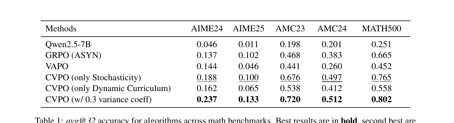
The headline numbers: CVPO’s full configuration improves over the second-best method by 9.3% (AIME24), 3.1% (AIME25), 25.2% (AMC23), 12.9% (AMC24), and 13.7% (MATH500) — relative improvements over whichever baseline is second-best on that column (sometimes VAPO, sometimes CVPO-only-Stochasticity). The two single-mechanism ablations (CVPO-only-Stochasticity and CVPO-only-Dynamic-Curriculum) both individually beat the VAPO baseline on every benchmark, which is the paper’s evidence that each mechanism contributes independently rather than one carrying the other. Interestingly, the stochasticity-aware correction alone is the stronger of the two individual mechanisms across the board — the paper attributes this to it “expanding the upper bound of model exploration,” though this is stated rather than further decomposed (it would have been useful to see, e.g., how much of the gap between only-Stochasticity and VAPO is attributable to the correct-trajectory suppression term vs. the incorrect-trajectory encouragement term individually).

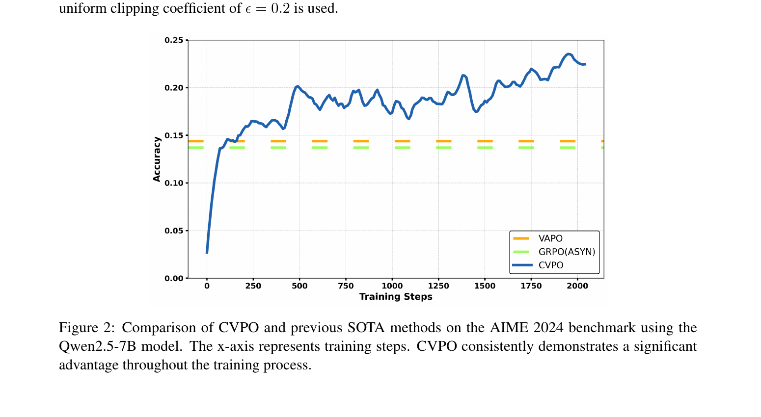
Figure 2’s shape is the paper’s strongest qualitative evidence for the curriculum mechanism specifically: VAPO and GRPO(ASYN) plateau (the dashed reference lines) well before 500 steps, while CVPO’s solid curve keeps climbing through 1500-2000 steps. The paper’s narrative interpretation is that CVPO’s early-phase medium-difficulty focus produces the fast initial rise, and the phase-switch to hard-question focus around the point where the baselines flatten out is what sustains the later gains — consistent with, though not conclusively isolated from, the curriculum-only ablation in Table 1.

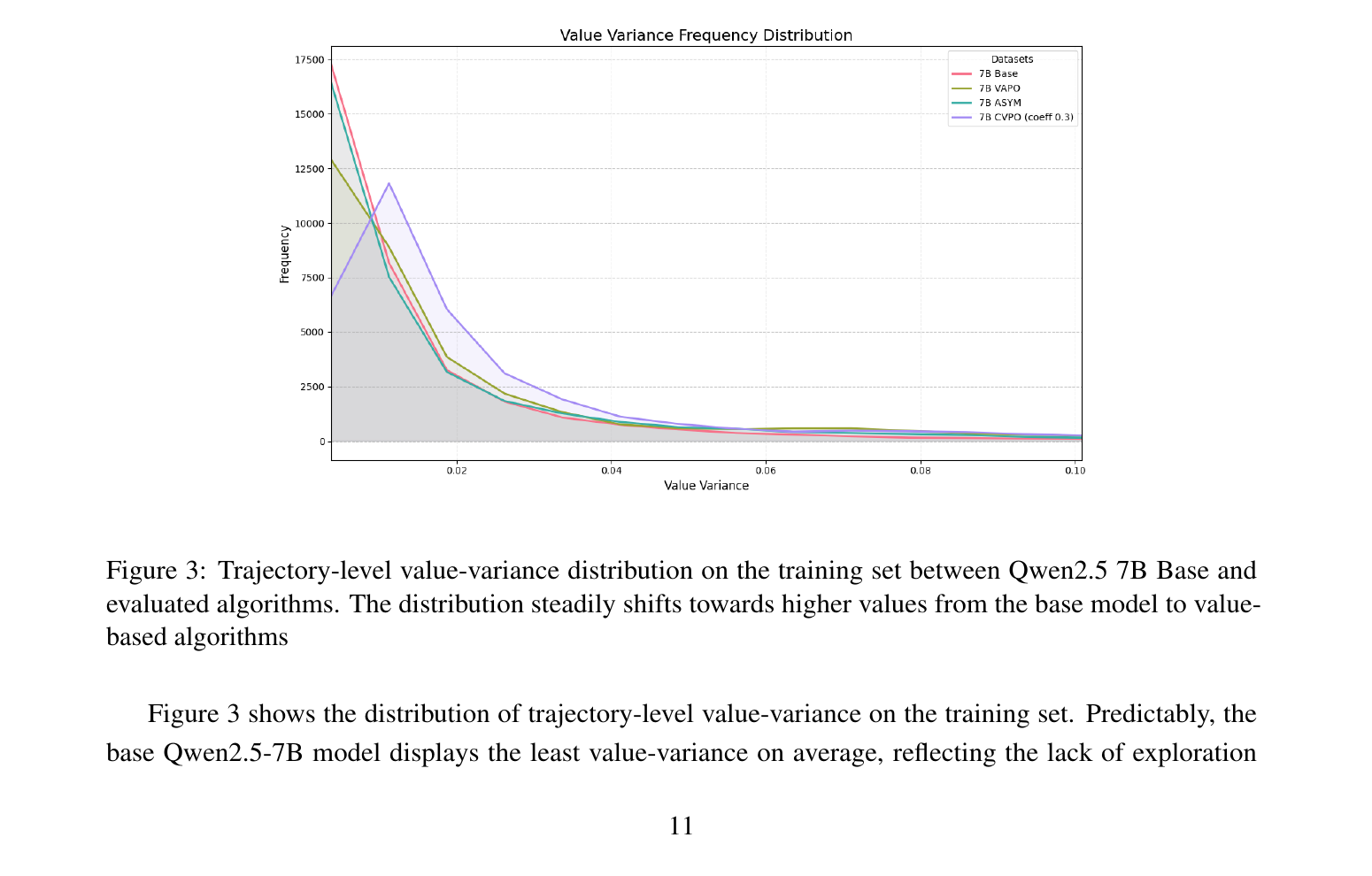
Figure 3 is the most direct empirical validation of the theoretical claim from Section 2: if CVPO’s mechanism is actually doing what the theory predicts, trained models should exhibit systematically higher trajectory-level value variance than baselines. That’s exactly the pattern shown — the base model, VAPO, and GRPO(ASYN) curves are nearly indistinguishable (peaking around variance $\approx 0.005$–$0.01$), while CVPO’s distribution has a visibly fatter right tail and a later peak ($\approx 0.01$–$0.015$), consistent with the intended effect of Eq. 15-16 systematically nudging trajectory variance upward for the trajectories that matter (largely the incorrect, low-variance ones being pushed to explore more). One reasonable question the paper doesn’t address: this is a training-set distribution measured post-hoc — a distribution of what variance patterns emerge from a trained policy, not a controlled counterfactual showing that variance causes the accuracy gain versus merely correlating with it.

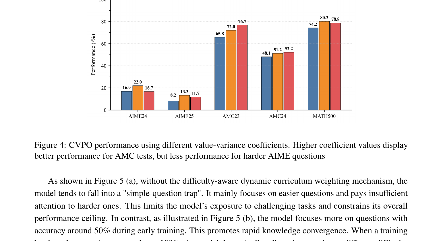
Figure 4 is the paper’s sensitivity/ablation study on the overall scale of the correction ($\alpha_P, \alpha_N$ scaled jointly by a single “coefficient”). The pattern is instructive and honest: pushing the coefficient higher (more aggressive variance-based correction) monotonically helps on the easier AMC benchmarks (65.8% → 72.0% → 76.7% on AMC23 as coefficient goes 0.1 → 0.3 → 0.5) but hurts on the harder AIME benchmarks past 0.3 (AIME24: 16.9% → 22.0% → 16.7%; AIME25: 8.2% → 13.3% → 11.7%). The paper’s explanation — larger coefficients mean larger effective advantage magnitudes, which means larger policy updates, which destabilizes the more delicate optimization needed for genuinely hard problems — is plausible and consistent with the Eq. 13 bound (bigger $\mathrm{Var}(V)$ manipulation → bigger permissible gradient norm → more risk of overshooting on problems where the “right” update direction is harder to estimate accurately in the first place). This is a real, disclosed limitation of the mechanism: there is no coefficient value that is simultaneously optimal across problem difficulties in this experiment, meaning the reported “CVPO (w/ 0.3 variance coeff)” headline numbers in Table 1 reflect one specific compromise point on this Pareto-like tradeoff, not a strictly dominant configuration.

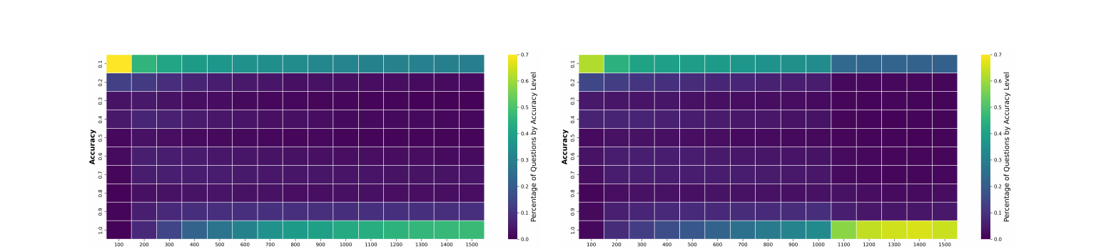
Figure 5 visualizes the curriculum mechanism’s intended effect directly: panel (a), without dynamic weighting, shows a persistent green/teal band along the bottom row (very-low-accuracy questions, $\rho_q \approx 0.1$) that never clears across 1500 steps — these are the “left behind” hard questions the fixed-weight scheme never prioritizes enough to actually solve. Panel (b), with the mechanism, shows the same bottom-row band gradually clearing after around step 1000-1100 as the bright yellow (high-fraction) region appears in the top row instead — meaning previously-stuck low-accuracy questions are being successfully pushed up into high-accuracy territory once the bottleneck-triggered reweighting kicks in. This is good qualitative evidence that the mechanism does what it says, though it’s worth noting the paper’s own prose describing panel (a) as the “simple-question trap” is slightly confusingly worded — the trap being illustrated is under-training on hard questions, not over-training on simple ones (the two are related but not identical framings of the same failure mode).

7. Limitations the paper states — and a few it doesn’t

The paper itself is fairly candid about one limitation: the value-variance coefficient tradeoff shown in Figure 4 (helps AMC, hurts AIME past a threshold) is presented directly, without spin. That’s good scientific practice and worth crediting.

Limitations the paper states less directly, or leaves for the reader to notice:

• Single model scale, single domain. All experiments use Qwen2.5-7B on math reasoning benchmarks. There is no evidence in the paper about whether the mechanism’s benefits hold at larger scale (e.g., 70B+, where value models are both more expensive to train and potentially better-calibrated to begin with, possibly changing the value-variance signal’s reliability), or on non-math reasoning domains with less clean binary reward (code generation with partial test-case credit, open-ended agentic tasks, multi-turn dialogue) where the “correct/incorrect” binary that underlies Eq. 15-16’s asymmetric weighting doesn’t cleanly exist.
• No wall-clock / compute-overhead accounting. The paper claims the mechanism is “cheap” (it is, computationally — Algorithm 1 and the Beta-posterior updates in Algorithm 2 are both $O(\text{batch size})$ operations with no extra forward/backward passes), but never reports actual wall-clock training time or GPU-hour comparisons against VAPO/GRPO(ASYN) to substantiate this. Given that CVPO trains for 2000+ steps to reach its reported gains (Figure 2), and the baselines plateau far earlier, a compute-normalized comparison (accuracy at matched GPU-hours, not matched steps) would be a fairer efficiency claim — right now it’s unclear whether CVPO’s advantage would look as strong if VAPO were simply trained for the same wall-clock budget instead of being read off its plateau.
• Sensitivity of the curriculum thresholds (0.3/0.05, 0.8/0.03) and the sigmoid shape constants ($k_1, c_1, k_2, c_2$ and primed variants) is never tested. As discussed in Section 4.1, these are stated as fixed constants with no ablation showing how much the results depend on them, unlike the variance coefficient which does get an ablation (Figure 4). This asymmetry in what gets ablated makes it hard to judge how brittle the curriculum mechanism specifically is to its many hand-tuned constants.
• The theoretical bound (Eq. 13) is an inequality relating variance to gradient magnitude only. It says nothing about gradient direction or about whether increasing $\mathrm{Var}(V)$ for a specific subset of trajectories (as CVPO does) actually improves the quality of the resulting updates rather than just their size. The empirical results (Table 1, Figure 3) are consistent with the mechanism working as intended, but the theory alone doesn’t guarantee this outcome — it’s necessary-but-not-sufficient scaffolding, and the paper doesn’t always clearly separate “this is proven” from “this is empirically observed to work.”
• Reward hacking / degenerate solutions around the variance signal are not discussed. Because $W_S$ directly scales the gradient magnitude based on a statistic ($\mathrm{Var}(V)$) computed from the same value model being trained, there’s a plausible failure mode where the value model learns to produce spuriously high or low variance patterns that game the weighting function rather than reflecting genuine exploration — a form of Goodhart’s law risk that isn’t addressed or ruled out empirically (e.g., no experiment tracks whether $\mathrm{Var}(V)$ starts correlating less with genuine exploration quality later in training as the value model potentially adapts to the correction mechanism it feeds into).

8. Critical analysis

Weaknesses and flaws specific to this paper. The strongest, most novel contribution — the theoretical bound in Eq. 13 linking $\mathrm{Var}(V)$ to gradient magnitude — is a genuinely useful piece of reasoning, but it’s a fairly weak (loose) bound built on two Cauchy-Schwarz applications and a worst-case covariance assumption, so its role is closer to “motivation for trying variance-based weighting” than “proof that this specific weighting scheme is correct.” The paper occasionally blurs this distinction in prose (e.g., in Section 6.1’s phrase “theoretical analysis proves that appropriately leveraging this variance can improve the upper bound of model performance” — this overstates what Eq. 13 actually shows, which is a bound on gradient norm, not a statement about the performance ceiling the model can reach). A reader skimming the abstract or conclusion could come away thinking the paper has a tight theoretical guarantee of improved outcomes, when what it actually has is a plausibility argument plus strong empirical results.

Limitations the authors understate or omit. As noted above, the compute-overhead accounting is essentially absent — a paper proposing a new training recipe for expensive LLM RL runs (64 A800s, 2000+ steps) should report wall-clock or GPU-hour comparisons, not just step-matched accuracy curves, especially when the comparison baselines visibly plateau far earlier than CVPO’s reported training horizon. There’s also an unaddressed circularity risk: the value model that measures $\mathrm{Var}(V)$ is the same value model being shaped by the training signal that $\mathrm{Var}(V)$ feeds into (via the advantage in Eq. 27), and the paper never investigates whether this creates any feedback loop that could degrade the reliability of the variance signal over long training runs — Figure 3’s variance-distribution shift is consistent with the mechanism “working,” but is equally consistent with the value model’s raw calibration drifting under a self-referential training signal, which the paper doesn’t distinguish.

Concrete, specific improvement suggestions.

1. Report GPU-hour-matched (not just step-matched) accuracy curves against VAPO and GRPO(ASYN), including the extra overhead (if any) of computing $\sigma_i, \mu_k$, and the Beta-posterior bookkeeping, to substantiate the “cheap” framing with numbers rather than asserting it.
2. Run an ablation over the sigmoid steepness parameters $\lambda_P, \lambda_N$ and the four curriculum shape constants ($k_1,c_1,k_2,c_2$ and their primed bottleneck-phase counterparts) analogous to the variance-coefficient ablation already in Figure 4 — right now these eight numbers are simply asserted, with no sensitivity analysis, despite the mechanism’s behavior depending on them just as much as on the coefficient that does get ablated.
3. Test whether the mechanism transfers to a domain with continuous/partial-credit rewards (code generation with test-case pass rates, rather than binary math correctness) — the entire asymmetric-weighting design in Eq. 15-16 hinges on a clean binary $R(\tau)\in\{0,1\}$ split, and it’s not obvious how to extend it gracefully to a reward that isn’t binary.
4. Add a direct diagnostic for the circularity concern: e.g., track the correlation between $\mathrm{Var}(V)$ and an independent exploration proxy (like token-level entropy, or an LLM-judge rating of “how many distinct solution strategies were considered”) over the course of training, to distinguish “the value model’s variance signal remains a faithful exploration proxy throughout training” from “the value model has adapted its variance output to game the weighting function it feeds.”

9. Reproducibility notes

The paper reports the full set of hyperparameters needed to reproduce the main experiment (Section 5.1): base model (Qwen2.5-7B), training data (DAPO-Math-17k), reward rule (exact match on \boxed{} or Answer:, +1/-1), optimizer (AdamW, actor LR $1\times10^{-6}$, critic LR $2\times10^{-6}$), batch composition (256 batch size, 16 rollouts/prompt, max 6144 response tokens), GAE settings ($\lambda_{\text{critic}}=0.1$, length-adaptive factor $\alpha=0.17$, $\gamma=1.0$), clip range ($\epsilon_{\text{lower}}=0.2$, $\epsilon_{\text{higher}}=0.28$), positive-LM-loss coefficient $\mu=0.1$, value-model warm-up (21 steps), and hardware (64 A800 GPUs). This is a reasonably complete list for reproducing the training run’s macro-configuration.

What is not fully specified for exact reproduction: the values of $\alpha_P, \alpha_N$ (the gain parameters in Eq. 15-16) are never given numerically in the main text — only the overall “variance coefficient” (0.1/0.3/0.5) ablated in Figure 4 is reported, and it’s not stated explicitly how that single coefficient maps onto $\alpha_P$ and $\alpha_N$ individually (are they scaled jointly and equally, or is there an implicit asymmetry preserved?). Similarly, $\lambda_P$ and $\lambda_N$ (sigmoid steepness) are described as “fixed” but no numeric values are given. No code repository link is provided in the paper as reviewed. A careful reproduction attempt would need to either contact the authors for the missing constants or re-derive reasonable values by grid search against the reported Table 1 numbers as a target — a non-trivial undertaking given how many interacting hyperparameters (variance coefficient, curriculum thresholds, sigmoid shape constants) the full method has.

10. Conclusion

CVPO makes a genuinely interesting observation — that a value model’s variance across a trajectory, not just its point estimate, carries useful signal about how much exploration actually happened — and backs it with a clean (if loose) theoretical bound connecting variance to policy-gradient magnitude. Combined with a Bayesian difficulty tracker that adapts curriculum weighting as the model’s own capability shifts the effective difficulty landscape, the resulting method shows consistent, sizable gains over VAPO and a hardened GRPO baseline on standard math-reasoning benchmarks with a 7B model, and — usefully — the paper is honest about at least one real tradeoff (the variance coefficient helping easier benchmarks while hurting harder ones past a threshold). The gaps that would most strengthen the work are exactly the kind that tend to get left for follow-up papers: compute-normalized comparisons, ablations over the many hand-tuned curriculum constants, and evidence the mechanism generalizes beyond single-scale, math-only, binary-reward settings. For anyone building an RL-for-reasoning pipeline today, the most portable takeaway is probably not “use CVPO exactly as specified” but the underlying idea that a trained value model already contains a second-order exploration signal worth extracting, cheaply, from statistics you’re already computing.