Bole: Efficient Tree Speculation for Hybrid-Attention Language Models

Review date: 2026-08-09 Author: Zhongzhu Zhou Paper reviewed: Bole: Efficient Tree Speculation for Hybrid-Attention Language Models Paper authors: Li Wang, Yi Su, Xiabao Wu, Chiran You, Yongchao Liu, Zhan Qiu, Juelu Zhang, Jiajun Zheng, Fangxin Liu, Jie Zhang, Chen Tian, Chengying Huan (Nanjing University, Ant Group, Shanghai Jiao Tong University, Peking University) arXiv: 2608.01651 Venue/Status: Preprint (cs.DC), August 2026

1. Why hybrid-attention models need a different speculative-decoding story

If you’ve followed LLM serving over the last two years, tree speculative decoding feels like a solved problem. EAGLE-2 and Medusa build a small drafter that proposes several candidate continuations at once, arranged as a tree instead of a flat sequence; the big target model scores every node of that tree in one parallel forward pass using an ancestor mask (a node can attend to its own ancestors on the tree, but not to sibling branches); and standard rejection sampling picks the longest accepted path without changing the model’s output distribution. Systems like SGLang and AdaServe have turned this into production infrastructure, and reported speedups of up to 5x are common.

The quiet assumption baked into every one of these systems is that the target model is a full-attention Transformer. Full attention has a wonderfully convenient property for tree verification: because every token attends to a KV cache that grows by simple concatenation, you can flatten the whole proposal tree into one long ancestor-masked sequence and score it with a single attention call, using a mask matrix to block sibling-to-sibling attention. The “state” a node needs (its KV cache) is just “all its ancestors’ keys and values, concatenated” — trivially parallel, because concatenation of independent vectors has no sequential dependency.

Recurrent linear attention breaks this property completely. Models like Qwen3.5 and Kimi Linear interleave full-attention layers with Gated DeltaNet (GDN) layers, which summarize the entire prefix into a single fixed-size matrix state $S_t \in \mathbb{R}^{d_k \times d_v}$ instead of a growing KV cache. This state is updated, not concatenated: $S_t$ is a function of $S_{t-1}$ plus the current token’s contribution. There is no “attention matrix” you can mask, because there is no attention matrix at all in the classical sense — the recurrence is the mechanism. If node B is a child of node A in the proposal tree, computing B’s linear-attention output requires A’s post-update state, which requires A’s parent’s state, and so on back to the last committed token. This is an intrinsically serial dependency chain, and it is precisely what full-attention tree verification tricks were designed to eliminate for full attention, but cannot eliminate here.

This paper — Bole — is about closing exactly this gap: making tree speculative decoding for hybrid full/linear-attention models as parallel and memory-cheap as it already is for pure full-attention models, without changing the math of what gets computed (the paper’s core claim, backed by a theorem, is that its reformulation is exactly equivalent to sequential execution, not an approximation).

Prerequisites: what you need to know before diving in

Autoregressive decoding and the memory-bound regime. When an LLM generates text token by token, each new token requires one full forward pass through the model. At small batch sizes, this forward pass is typically memory-bandwidth bound: the GPU spends most of its time transferring model weights from HBM to on-chip memory, and comparatively little time actually computing with them, because there’s only one token’s worth of arithmetic to do per weight load. This creates significant unused compute (“FLOPs”) headroom — the same headroom that speculative decoding exploits.

Speculative decoding, in one paragraph. Instead of generating one token per forward pass, use a cheap “drafter” model (often a lightweight auxiliary head trained via multi-token prediction, or a separate small model) to propose several candidate future tokens at once. Then run the expensive “target” model once over all the candidates in parallel — since a forward pass over $k$ tokens costs barely more than a forward pass over 1 token in the memory-bound regime, you get $k$ tokens’ worth of verification for close to the price of 1. A sampling procedure (originally due to Leviathan et al. and Chen et al.) then accepts a prefix of the candidates that is statistically consistent with what the target model itself would have generated, guaranteeing the output distribution is unchanged, and corrects the first rejected position by resampling from the target’s own distribution.

From flat speculation to tree speculation. A single linear chain of candidate tokens wastes opportunities: if the drafter is unsure between two plausible continuations, proposing only one throws away the other. Tree speculation (Medusa, EAGLE-2, Sequoia) has the drafter propose a branching tree of candidates rather than a single chain, and has the target model verify the entire tree in one forward pass, using an ancestor mask so that each node only “sees” its own path back to the root, not sibling branches it has no business attending to. Because more of the tree’s paths turn out to overlap with what the target model would actually generate, tree speculation reliably lands more mean accepted tokens (MAT) per round than flat speculation — EAGLE-2 reports 4–5.5 accepted tokens per round.

Gated Delta Networks (GDN) and the gated delta rule. GDN is a modern linear-attention variant (Yang, Kautz & Hatamizadeh, “Gated Delta Networks: Improving Mamba2 with Delta Rule”) that maintains, per attention head, a fixed-size matrix state $S_t \in \mathbb{R}^{d_k \times d_v}$ instead of a per-token KV cache. At each step $t$ it applies a decay gate $\gamma_t$, computes a “delta” correction $u_t$ between the new value and what the current state would predict, and folds that correction into the state with an outer product:

$$\widetilde{S}_t = \gamma_t S_{t-1}, \qquad u_t = \beta_t (v_t - \widetilde{S}_t^\top k_t),$$ $$S_t = \widetilde{S}_t + k_t u_t^\top, \qquad o_t = S_t^\top q_t. \tag{1}$$

Here $q_t, k_t \in \mathbb{R}^{d_k}$ are the query/key vectors, $v_t, u_t, o_t \in \mathbb{R}^{d_v}$ are the value/correction/output vectors, $\gamma_t > 0$ is a decay gate (how much of the old state to keep), and $\beta_t$ is a write gate (how strongly to apply the new correction). The state $S_t$ is a compressed, fixed-size summary of everything seen through token $t$: $O(1)$ in sequence length, versus $O(L)$ for a full-attention KV cache growing with prompt length $L$. This is the entire reason hybrid models exist — you trade some of full attention’s unbounded lookback for a bounded, cheap-to-maintain state — but it is also exactly why tree speculation over GDN layers is hard: $S_t$ literally depends on $S_{t-1}$, with no way to “concatenate around” that dependency the way full attention lets you concatenate KV entries.

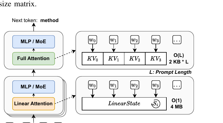
Figure 1 (paper Fig.2): Full attention retains one KV pair per prefix token, growing as $O(L)$ in memory (roughly 2 KB per token per layer in the paper’s setting); GDN instead compresses the entire prefix into one fixed-size state matrix, $O(1)$ in sequence length (about 4 MB per layer). Both feed the same next-token prediction pipeline, but their history representations — and therefore what “extending the tree by one node” means computationally — are fundamentally different.

2. Three concrete bottlenecks, quantified

Before presenting the fix, the paper spends real effort measuring exactly how existing systems fail on hybrid models, rather than jumping straight to the proposed mechanism. This matters because it tells you which design choices are load-bearing and which are incidental.

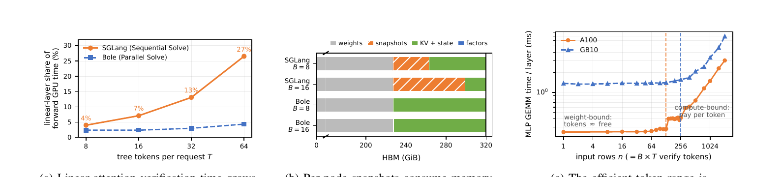
Figure 2 (paper Fig.1): (a) Linear-attention verification time as a share of the total forward pass grows from 4% to 27% as the tree expands from 8 to 64 nodes under naive sequential recurrence, while Bole’s parallel solve stays flat below 5%. (b) Per-node state snapshots consume tens of GiB of HBM and crowd out KV-cache/serving capacity; Bole’s factorized representation uses a small, fixed sliver instead. (c) The “additional tokens are nearly free” region of the roofline model is hardware-specific — the transition to compute-bound execution happens near 128 rows on A100 but 256 rows on GB10 (NVIDIA’s DGX Spark with the GB10 Grace Blackwell superchip), so a fixed verification budget tuned for one GPU is wrong on another.

L1 — Serial recurrence. Existing engines (e.g., SGLang’s native GDN tree path) apply Eq. (1) one tree node at a time, because each node needs its parent’s post-update state before it can compute its own. A tree with $T$ proposal nodes therefore requires $T$ sequential recurrent steps, even though every proposal token’s inputs ($q, k, v$, gates) are already fully known before the target forward begins — the data is available in parallel, but the classical recurrence formula forces the computation to be serial. Measured on Qwen3.5-9B/A100, this raises the linear-attention layers’ share of total forward-pass time from 4% (8-node tree) to 27% (64-node tree) — a scaling behavior that directly fights against the entire point of tree speculation, which is to make bigger trees (more candidate tokens verified per round) nearly free.

L2 — State-snapshot explosion. Before sampling resolves which branch gets accepted, existing systems don’t know which candidate node’s state will actually matter, so they conservatively materialize a complete post-update GDN state for every tree node — one full $d_k \times d_v$ matrix per head, per node. This is $\Theta(T \cdot H \cdot d_k \cdot d_v)$ space, growing linearly in both tree size $T$ and (because you’re doing this for every request in the batch) batch size $B$. Concretely, for Qwen3.5-122B-A10B at $T=32$ tree nodes, this snapshot storage is 36 GiB at batch size 8 and 72 GiB at batch size 16 — displacing KV-cache and active-request capacity that would otherwise expand serving throughput.

L3 — Hardware-dependent, non-transferable verification capacity. The paper invokes the standard roofline model: at small numbers of verification rows $n$, a GEMM (the dominant cost inside MLP/attention layers) is bandwidth-bound, so the extra work of verifying more tree tokens is “nearly free” — you’re paying for the weight transfer regardless, and adding rows barely changes the wall-clock time. Beyond a hardware-specific threshold, the same GEMM becomes compute-bound and latency starts growing roughly linearly with row count. That threshold is not a property of the model alone — it’s a joint property of the model, the GPU’s compute-to-bandwidth ratio, and (for a full hybrid forward) the current KV length and tree shape. A verification budget tuned once and hardcoded (as most tree-speculation systems effectively do) will be systematically wrong on a different GPU, or even on the same GPU under a different batch/KV-length regime.

These three limitations trace back to three genuinely different challenges that span algorithm, kernel, and runtime design: (1) tree-coupled recurrent dependencies that an ancestor mask cannot remove (since there’s no attention matrix to mask), (2) state divergence before the runtime knows which branch will be accepted, and (3) a per-request verification cost that depends on hardware and current serving conditions rather than being a fixed constant. Bole addresses all three with one coherent kernel–runtime co-design.

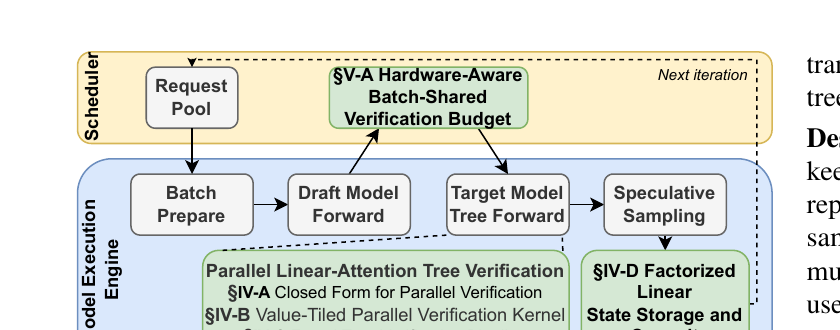
Figure 3 (paper Fig.4): Bole’s end-to-end pipeline. A hardware-aware, batch-shared verification budget (top) feeds into per-round batch preparation, drafter forward, target-model tree forward, and speculative sampling. Inside the target forward, Bole’s parallel linear-attention tree verification (closed-form solve + value-tiled kernel) replaces the sequential recurrence, and a factorized linear-state storage/commit mechanism replaces full per-node snapshots. The whole loop is integrated into SGLang.

3. Deriving the closed form: turning a serial recurrence into one matrix solve

This is the mathematical heart of the paper, and it deserves to be unpacked slowly, because the result is genuinely elegant once you see why it works.

3.1 Setting up notation

Consider one proposal tree with $T$ nodes, and let $\pi(i)$ denote the parent of node $i$ (with $\pi(i) = 0$ meaning “child of the committed root,” whose pre-tree state is $S_{\mathrm{pre}}$). For a node $i$, let $A(i)$ be the set of its strict draft ancestors (all nodes on the root-to-$i$ path, excluding $i$ itself), and let $d$ be the maximum size of $A(i)$ over all nodes — i.e., the tree’s maximum depth. Stack every node’s operands into matrices $Q, K \in \mathbb{R}^{T \times d_k}$ and $V \in \mathbb{R}^{T \times d_v}$, with row $i$ equal to $q_i^\top, k_i^\top, v_i^\top$ respectively; similarly stack the gates into vectors $\beta, \gamma \in \mathbb{R}^T$.

Define the cumulative decay along a path, $P_i = \prod_{r \in A(i) \cup \{i\}} \gamma_r$ — literally just applying the sequential recurrence’s decay gate along the whole chain from the root to node $i$. Stack these into $P = (P_1, \ldots, P_T)^\top$ and let $D_P = \mathrm{diag}(P)$, $D_\beta = \mathrm{diag}(\beta)$.

3.2 Lemma 1: every path state has a closed form

The first structural step is to notice that if you unroll the sequential update in Eq. (1) along one root-to-node path, the dependence on ancestors telescopes into a sum, not a nested recursion. Concretely:

$$\widetilde{S}_i = P_i S_{\mathrm{pre}} + \sum_{j \in A(i)} \frac{P_i}{P_j} k_j u_j^\top, \qquad S_i = P_i S_{\mathrm{pre}} + \sum_{j \in A(i) \cup \{i\}} \frac{P_i}{P_j} k_j u_j^\top. \tag{3}$$

Why this is true, step by step. Expand $S_{\pi(i)}$ one level and multiply by $\gamma_i$: you pick up a factor $\gamma_i$ times whatever $S_{\pi(i)}$ already was. Doing this recursively down to the root, the gate factors compound multiplicatively — that’s exactly what $P_i / P_j$ captures: the residual decay between the state that existed right after node $j$ was processed, and the state that exists right after node $i$‘s ancestor chain finishes decaying it further. Topological induction (processing nodes in parent-before-child order) makes this rigorous. Reading out this state with a query $q_i$ gives:

$$o_i^\top = P_i\, q_i^\top S_{\mathrm{pre}} + \sum_{j \in A(i) \cup \{i\}} \frac{P_i}{P_j}(q_i^\top k_j)\, u_j^\top. \tag{4}$$

The intuition: node $i$‘s output is a decayed readout of the shared pre-tree state, plus a weighted sum of every ancestor’s correction term $u_j$, where the weight is exactly the kind of decayed key-similarity term $(q_i^\top k_j)$ you’d expect from an attention-like mechanism, scaled by the residual decay ratio.

3.3 Lemma 2: stacking corrections into one linear system

Eq. (4)‘s coefficient of $u_j$ is exactly what the paper calls $C_{ij}$ — so stacking Eq. (4) over all $T$ nodes gives $O = D_P Q S_{\mathrm{pre}} + CU$, where $U$ stacks every node’s correction vector $u_i^\top$. But $U$ itself is defined recursively (via $u_i = \beta_i(v_i - \widetilde{S}_i^\top k_i)$, and $\widetilde{S}_i$ depends on ancestors’ $u_j$ through Eq. (3)) — so we haven’t actually removed the recursion yet, we’ve just relocated it into solving for $U$. Substituting Eq. (3) into the definition of $u_i$ and rearranging, the paper shows this recursion becomes one linear system:

$$(I + G)\, U = R, \qquad G_{ij} = \beta_i \frac{P_i}{P_j} k_i^\top k_j \;\; (j \text{ a strict ancestor of } i), \qquad R = D_\beta\left(V - D_P K S_{\mathrm{pre}}\right). \tag{5}$$

Here $R$ is precisely the local delta each node would compute against a purely pre-tree-decayed readout — i.e., “what correction would node $i$ apply if none of its ancestors had contributed anything extra.” $G$ then captures exactly the extra correction that flows in from ancestors: $G_{ij}$ is nonzero only when $j$ is a strict ancestor of $i$ (enforced by construction, using the ancestor mask $M^-$), so under a parent-before-child node ordering, $G$ is strictly lower triangular — every entry above or on the diagonal is exactly zero.

3.4 Lemma 3: why a lower-triangular tree matrix is easy to invert

This is the key trick that makes the whole approach practical rather than just theoretically elegant. A strictly lower-triangular matrix restricted to a tree structure (rather than a general lower-triangular matrix, which would need $O(T^3)$ Gaussian elimination or $O(T^2)$ forward substitution) is nilpotent with a very small nilpotency degree: a nonzero entry of $G^m$ corresponds to an “$m$-edge ancestor path” in the tree, and no such path can be longer than the tree’s maximum depth $d$. So $G^{d+1} = 0$, and by the standard geometric-series identity for nilpotent matrices:

$$(I+G)^{-1} = \sum_{m=0}^{d} (-G)^m. \tag{6}$$

Because typical speculative-decoding trees are shallow (depth $d \approx 4$–$8$, since drafters only look a handful of tokens ahead), this sum has only a handful of terms — turning what looks like an expensive general matrix inversion into a finite polynomial with $d{+}1$ terms, each of which is just one matrix-vector product $GZ$. This is the load-bearing insight: it’s not that solving $(I+G)U=R$ is asymptotically cheap in general (in general, triangular solves already are, at $O(T^2)$) — it’s that for a tree-shaped $G$, the polynomial degree is bounded by tree depth rather than tree size $T$, so the solve parallelizes into $d$ rounds of independent matrix multiplies rather than $T$ rounds of sequential updates.

3.5 Theorem 1: the full closed form

Putting the three lemmas together:

$$O = D_P Q S_{\mathrm{pre}} + C(I+G)^{-1} D_\beta\big(V - D_P K S_{\mathrm{pre}}\big). \tag{2}$$

The paper states, and proves via the lemma chain above, that this identity is algebraically exact — not an approximation of the sequential recurrence, but a rearrangement of the same computation into a form with no node-wise traversal. Every quantity on the right ($D_P, Q, S_{\mathrm{pre}}, C, G, D_\beta, V, K$) is knowable before any node’s output is computed, because it only depends on the (already fully known) tree topology, gates, and $Q/K/V$ — none of it depends on any other node’s output. That’s what converts an inherently sequential recurrence into one shared linear system that can be solved for all $T$ nodes simultaneously.

3.6 Bole’s parallel-verification algorithm, step by step

Putting this into an explicit numbered procedure (as required by clause 15a — the paper describes this as “Design 1,” and we make the implicit steps concrete):

Algorithm 1: Bole closed-form parallel tree verification (per layer, per head)

Input: proposal tree topology (parent map π, ancestor mask M⁻),
       stacked Q, K, V ∈ R^{T×d}, gates β, γ ∈ R^T, pre-tree state S_pre
Output: node outputs O ∈ R^{T×d_v}, correction factors U ∈ R^{T×d_v}
                                                (to be committed later)

1.  Compute path-cumulative decay: P_i ← ∏_{r ∈ A(i)∪{i}} γ_r  for every node i
    (a simple prefix product walked once along each root-to-node path;
     can be computed for all nodes in O(d) parallel rounds via
     doubling, or O(T) with one topological pass — not the bottleneck).
2.  Form D_P ← diag(P), D_β ← diag(β).
3.  Compute Gram matrices  KKᵗ ← K Kᵗ,  QKᵗ ← Q Kᵗ   (batched matmul).
4.  Apply the ancestor mask to build the tree-interaction matrices:
        G ← D_β D_P [ (KKᵗ) ⊙ M⁻ ] D_P⁻¹        (strictly lower-triangular)
        C ← D_P     [ (QKᵗ) ⊙ M⁺ ] D_P⁻¹        (M⁺ = M⁻ + I)
5.  Compute the pre-tree readout and local delta:
        B₀ ← D_P (Q S_pre)
        R  ← D_β ( V − D_P (K S_pre) )
6.  Solve (I + G) U = R via the finite Neumann series (Lemma 3):
        Z⁽⁰⁾ ← R;  U ← R
        for m = 0 to d−1:
            Z⁽ᵗ⁺¹⁾ ← −G Z⁽ᵗ⁾          # one matmul per round, all T nodes at once
            U ← U + Z⁽ᵗ⁺¹⁾
        # after d rounds, U is EXACTLY (I+G)⁻¹R  (Lemma 3 guarantees this
        # is exact, not an approximation, because G^{d+1} = 0)
7.  Compute final readout:  O ← B₀ + C U
8.  Return O (feeds sampling) and U, P, K (feeds the factorized-state
    commit mechanism in §5 — NOT a full T-node state snapshot)

Every step above operates on all $T$ nodes at once — steps 1, 3–7 are matrix/tensor operations with no per-node sequential loop (step 1’s prefix product is the one place with a topological dependency, but it is $O(d)$ deep, not $O(T)$ deep, and is cheap relative to the Gram-matrix and Neumann-series matmuls). This is what “solves L1” concretely means: the $T$-step sequential chain from the naive implementation becomes a fixed $d$-round loop of matrix multiplies, where $d$ (tree depth, typically ≤ 8) is far smaller than $T$ (tree size, up to 64+ in the paper’s experiments).

4. Mapping the math onto silicon: the value-tiled kernel

A closed form is only useful if it maps efficiently onto a GPU’s execution model. This is “Design 1“‘s second half, and it’s where the paper gets genuinely systems-y.

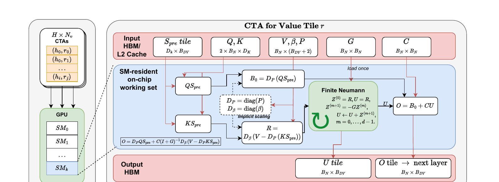
Figure 4 (paper Fig.5): One cooperative thread array (CTA) processes one value tile $r$ of width $b_v$, covering the full tree extent $\widetilde{T}$. It loads $S_{\mathrm{pre}}$, $Q/K$, $V/\beta/P$, and the pre-built factors $G, C$ from HBM/L2 once, forms $QS_{\mathrm{pre}}$ and $KS_{\mathrm{pre}}$, runs the finite-Neumann recurrence entirely in on-chip working memory, and only writes the final $U$ and $O$ tiles back to HBM.

Why value-domain decomposition, not tree-domain decomposition? The naive approach would be to map the whole tree extent $\widetilde{T}$ (the fixed kernel width covering the tree) to one CTA, processing all $d_v$ value channels together. But this would require $\Theta(\widetilde{T}^2 + \widetilde{T} d_v + d_k d_v)$ of on-chip storage per CTA and expose only one schedulable CTA per attention head — far too little parallelism to fill a modern GPU’s dozens of streaming multiprocessors (SMs). The key observation the paper exploits: the tree-interaction factors $G, C \in \mathbb{R}^{T \times T}$ depend only on tree topology, $Q/K$, and gates — not on which value channel you’re computing. So Bole partitions the $d_v$ value columns into $N_v = \lceil d_v / b_v \rceil$ tiles of width $b_v$, computes $G, C$ once per layer/head (amortizing the $O(\widetilde{T}^2 d_k)$ Gram-matrix construction cost across all $N_v$ tiles), and assigns each value tile to its own independently schedulable CTA. This directly multiplies available parallelism by $N_v$ without duplicating the expensive part of the computation.

Why also tile along the key dimension $d_k$? Value tiling alone doesn’t bound the other large intermediate: each value tile still needs to contract against the full key dimension $d_k$ to form $QS_{\mathrm{pre}}$ and $KS_{\mathrm{pre}}$. Bole further chunks this dimension into $b_k$-wide pieces and streams them through a single-stage software pipeline, so only the current $Q/K$ chunk and the matching slice of $S_{\mathrm{pre}}$ need to be resident at any instant, rather than the entire $d_k \times b_v$ state tile.

Design-choice discussion — the $(b_k, b_v)$ tradeoff. This is exactly the kind of non-trivial design choice clause 15c asks to be made explicit:

• Larger $b_v$: amortizes the fixed per-CTA setup cost (loading $G, C$, launching the kernel) over more value channels, but enlarges the persistent $R/Z/U$ and accumulator register/shared-memory tiles, and creates fewer independent CTAs — hurting occupancy on GPUs with many SMs to fill.
• Smaller $b_v$: reduces each CTA’s register/shared-memory footprint and exposes more schedulable parallelism, but duplicates the fixed setup/factor-loading overhead across more, narrower tiles — wasted work if $N_v$ grows too large relative to the number of SMs.
• Larger $b_k$: coarser tensor-core MMA (matrix multiply-accumulate) work per chunk, fewer partial-accumulation rounds, but a bigger transient shared-memory footprint per chunk.
• Smaller $b_k$: the opposite tradeoff — lower footprint, more chunks, more loop overhead.

The paper doesn’t claim a universal optimum; it selects $(b_k, b_v)$ from a small set of compile-time configurations and empirically balances resource usage against concurrency, bounding one CTA’s working set at $M_{\mathrm{CTA}} = \Theta\!\big(\widetilde{T}^2 + \widetilde{T} b_v + b_k(\widetilde{T}+b_v)\big)$ while creating $H N_v$ independently schedulable CTAs per request (where $H$ is the number of attention heads). This is a classic GPU-kernel tension — per-thread-block efficiency versus SM occupancy — made concrete for this specific recurrence structure.

On-chip finite-Neumann execution (mapping Algorithm 1 step 6 to hardware). Once inside one CTA, the $d$-round Neumann series from Algorithm 1’s step 6 executes entirely in on-chip registers/shared memory: $Z^{(0)} = R^{(r)}$, then $Z^{(m+1)} = -GZ^{(m)}$, $U^{(r)} \mathrel{+}= Z^{(m+1)}$ for $m = 0, \ldots, d-1$, where each $GZ^{(m)}$ decomposes into tensor-core MMA fragments along the node-reduction dimension. Because $d$ (tree depth) is small and fixed at compile time, this loop unrolls into a small, regular sequence of tensor-core operations with zero intermediate HBM traffic — $B_0^{(r)}$, $R^{(r)}$, and every $Z^{(m)}$ live and die entirely on-chip; only the final $O^{(r)}$ tile (for sampling) and the $U^{(r)}$ tile (for state commit) ever leave the CTA. The paper reports this design increases achieved GPU occupancy by 3.6x–7.9x and L1/shared-memory throughput by 1.8x–4.1x relative to the naive sequential kernel, translating directly into the 3.4x–7.7x complete-verification-core speedup measured in §6 below.

5. The other half of the problem: factorized speculative-state lifecycle

Solving L1 (serial recurrence) doesn’t automatically solve L2 (state-snapshot explosion) — you could imagine a parallel solver that still ends up materializing a full state per node. Bole’s second design (“Design 2”) avoids this by observing something specific to how Lemma 1 represents states.

5.1 Why full snapshots are wasteful, formalized

Recall Lemma 1: $S_i = P_i S_{\mathrm{pre}} + \sum_{j \in A(i) \cup \{i\}} \frac{P_i}{P_j} k_j u_j^\top$. This says every node’s full state $S_i \in \mathbb{R}^{d_k \times d_v}$ is completely determined by (a) the single shared $S_{\mathrm{pre}}$, and (b) a small set of rank-one update factors $(P_j, k_j, u_j)$ along its own path. Materializing $T$ full states costs $\Theta(T H d_k d_v)$ space — quadratic in the per-head state dimension $d_s$ if $d_k = d_v = d_s$. But storing just the factors that generate those states costs only:

$$\Theta(H d_k d_v) + \Theta\big(T H (d_k + d_v + 1)\big). \tag{9}$$ $$\underbrace{\phantom{X}}_{\text{committed state}} \qquad \underbrace{\phantom{XXXXXXXXXXXXXXXXX}}_{\text{tree factors, linear in } d_s \text{ not } d_s^2}$$

When $d_k = d_v = d_s$, a full per-branch state costs $\Theta(H d_s^2)$ elements, while one factorized node costs only $\Theta(2 H d_s)$ — the savings ratio grows with the state dimension itself, not with any particular tree shape. This is why the measured savings in Table I (57–151 MB for Bole’s factors versus 4.7–14.1 GB for full snapshots, at $T=100$) are so large: $d_s$ is not small in modern hybrid models.

5.2 The state lifecycle, as an explicit procedure

Figure 5: The factorized state lifecycle (§IV-D, “Factorized Linear State Storage and Commit” box in the architecture diagram) sits alongside the parallel verification kernel inside the target-model tree forward, and feeds a cross-layer batched commit step after speculative sampling resolves the accepted path.

Algorithm 2: Factorized speculative-state lifecycle (per request, per round)

Phase A — Verification (read-only w.r.t. canonical state):
1. Read the single immutable committed state S_pre for this request/layer
   from its HBM slot (canonical [H, d_v, d_k] layout). Do NOT copy it.
2. Run Algorithm 1 to obtain, for every candidate node i:
       - output O_i               (consumed by target-model sampling)
       - correction factor U_i     (kept, NOT expanded into a full S_i)
   Also retain per-node (P_i, K_i) — together (P, K, U) are the
   "tree factors" of Eq. (9). No node's full state is ever formed.

Phase B — Sampling (host/device, decides which branch "wins"):
3. Standard rejection sampling over the tree (using target vs. draft
   probabilities) selects one terminal accepted node a, defining the
   accepted path P(a) = A(a) ∪ {a}.
4. Rejected branches: DISCARD their (P, K, U) factors. No rollback,
   no state-cache slot was ever allocated for them (nothing to free).

Phase C — Commit (only the accepted path is materialized):
5. Compact the accepted path's factors in topological order:
       K_a ∈ R^{|P(a)|×d_k},  U_a ∈ R^{|P(a)|×d_v},
       D_a = diag(P_a / P_j)_{j ∈ P(a)}
6. Reconstruct the ONLY state that must persist, via Lemma 1:
       S_new = P_a S_pre + (D_a K_a)^T U_a          # Eq. (10)
   This is exactly one batched tensor-core matmul.
7. Overwrite the request's HBM state slot with S_new (in place; old
   S_pre remains readable by any in-flight consumer until this write
   completes — no snapshot or copy-on-write slot is needed).
8. If no draft token was accepted this round, skip steps 5–7 entirely:
   the slot simply retains S_pre unchanged.
9. Fold this per-layer commit into ONE device-wide launch across all
   recurrent layers (since the accepted path P(a) is shared across
   layers), overlapping with the full-attention layers' ordinary KV
   cache commit (handled natively by SGLang).

The critical property that makes this correct is one the paper is explicit about: $S_{\mathrm{pre}}$ is never mutated during verification. Every candidate branch reads the same immutable $S_{\mathrm{pre}}$ and produces its own independent factors; nothing needs to “fork” a private copy of the state, and nothing needs a rollback mechanism, because nothing was ever tentatively written in the first place. This is the structural reason rejected branches are free to discard (step 4) — there is no mutable state to undo.

Measured impact. Table I in the paper reports this reduces transient per-request state memory by 82x–99x relative to full snapshots across four model sizes and two tree depths ($T=100, 200$). The paper’s ablation (§6G, discussed in §8 below) attributes the largest single component of Bole’s end-to-end online-serving gain to this mechanism specifically — more than either the parallel solver or the hardware-aware budget alone — because freeing tens of GiB of HBM directly translates into more KV-cache capacity, which in turn improves prefix-cache hit rates and reduces repeated prefills under continuous batching.

6. Design 3: turning L3 into a calibrated, batch-shared budget

Designs 1 and 2 make verification cheap; Design 3 decides how much verification to buy, and which candidate nodes get to spend that budget. This addresses L3 (hardware-dependent capacity) directly.

Why not just pick a fixed tree size? The paper models complete target-forward latency for verifying $N = \sum_i n_i$ total selected nodes across the batch (with per-request node count $n_i$, committed KV length $L_i$, tree depth $d_i$) as a sum of four terms:

$$T_{\mathrm{ver}}(\mathbf{n}, \mathbf{L}, \mathbf{d}) = T_{\mathrm{full}}(\mathbf{n}, \mathbf{L}) + T_{\mathrm{linear}}(\mathbf{n}, \mathbf{d}) + T_{\mathrm{dense}}(N) + T_{\mathrm{other}}(N). \tag{11}$$

Each term scales differently: full-attention layers’ KV work depends on both node count and KV length; linear layers (now cheap, thanks to Designs 1–2) depend on node count and tree depth; the shared MLP/projection layers batch all $N$ nodes together and can cross from bandwidth-bound to compute-bound execution partway through, at a point that depends on the GPU. The design-choice tension here: a node-count-only cost model (“verify at most $k$ nodes per request”) is simple to implement but ignores that the same node count $n_i$ can imply very different actual latency depending on $L_i$, $d_i$, and the GPU’s roofline knee — exactly the failure mode quantified in Fig. 2(c) above.

Algorithm 3: hardware-aware batch-shared verification budget

Offline (one-time calibration, per execution configuration c
          = {model, GPU/parallelism setup, batch-size bucket,
             KV-length bucket, tree-depth/template bucket}):
1. Sweep candidate total node counts N over the statically supported
   CUDA-Graph capacities G.
2. For each N ∈ G, measure T_ver(N | c): latency of the COMPLETE
   hybrid target forward (full attention + linear attention + MLP +
   TP communication + graph-capture effects) — not a per-component
   estimate, the real end-to-end number.
3. Measure T_dec(c): latency of ordinary one-token-per-request decoding
   under the same configuration (the "do nothing extra" baseline).
4. Select the largest calibrated capacity that stays within an
   admitted latency-overhead tolerance ε:
       B_ver(c) = max { N ∈ G : T_ver(N | c) ≤ (1+ε) T_dec(c) }   (12)
5. Store B_ver(c) in a lookup table indexed by configuration bucket.

Online (every decoding round):
6. Identify the current configuration bucket c from batching metadata
   (batch size, KV-length bucket, tree template in use).
7. Retrieve the pre-calibrated batch-shared capacity B_ver(c).
8. For every candidate node v with root-to-v path P(v), compute its
   cumulative draft probability:
       ρ(v) = ∏_{u ∈ P(v)} p_draft(u | π(u))
   (probability the DRAFTER assigns to reaching v along its whole path)
9. Always retain the root child of every active request's tree
   (fairness floor — no request is starved of any verification).
10. Fill the REMAINING capacity with the globally highest-ρ(v) nodes
    across the entire batch, using fixed-shape device top-k + scatter
    (stays inside the captured GPU iteration, no host round-trip).
11. Because a descendant's cumulative probability can never exceed its
    parent's (ρ is monotonically non-increasing down any path), the
    selected set per request is AUTOMATICALLY prefix-connected —
    no separate tree-repair pass is needed after top-k selection.

Design-choice discussion. The obvious alternative to step 2 (measuring the complete forward) is a per-component analytical cost model — estimate $T_{\mathrm{full}}$, $T_{\mathrm{linear}}$, $T_{\mathrm{dense}}$ separately from FLOPs/bytes counts and sum them. This would be far cheaper to calibrate (no profiling sweep needed) but the paper implicitly rejects it: kernel fusion, tensor-parallel communication overlap, and CUDA-Graph bucket effects interact non-additively in practice, so an analytical sum would systematically mis-predict the true knee point. The tradeoff is calibration cost (one-time, offline, amortized across the serving lifetime of a deployment) versus prediction fidelity (needs to be measured empirically per hardware/model/parallelism combination) — a reasonable choice for a production system that is deployed once and serves for a long time, less reasonable if you needed to support rapid, ad-hoc reconfiguration across many different hardware SKUs without re-profiling.

Boundary condition worth flagging: $\epsilon$ (the admitted latency-overhead tolerance in Eq. (12)) is a user-set knob that directly trades decode-latency overhead for mean-accepted-tokens (MAT) gain — the paper doesn’t report a sensitivity sweep over $\epsilon$ itself (only over total tree tokens, Fig. 11), so how sensitive the system is to a poorly chosen $\epsilon$ across different deployment SLOs is not directly shown.

7. Production integration: making the theory survive contact with SGLang

Theorem 1 plus Algorithms 1–3 describe an idealized computation; §V-B of the paper (≈ 6.2 kLoC of Python/Triton) covers the engineering needed to make this run inside a real, continuously-batching production serving engine without host-side stalls:

• CUDA Graph-native packed-forest execution. Variable-sized, per-request proposal trees are packed into one device-resident flat-ragged forest (request offsets + parent indices + compact ancestor metadata) rather than padded to a fixed shape. A request-aware block map then emits only the verification tiles that are actually internal to each request, so compacting the representation also reduces the work fed to the recurrent kernels — not just a memory-layout convenience.
• Unified cross-layer state commit. Each recurrent layer writes its (P, K, U) factors into a fixed slice of one shared, preallocated GPU buffer; after sampling produces one accepted-path descriptor per request, a single batched launch consumes those descriptors across every recurrent layer at once to evaluate Eq. (10), while SGLang’s native mechanism separately commits the matching full-attention KV entries. One launch, not one-per-layer.
• Bubble-free GPU execution. Selection, forest packing, target execution, sampling, path compaction, and state commit are captured as one GPU execution flow, eliminating host-induced synchronization stalls between these stages and letting the CPU scheduler prepare the next round’s work while the GPU finishes the current one.

This section is a useful reminder that a correct closed-form algorithm and an efficient kernel are necessary but not sufficient for a real speedup — without CUDA-Graph-compatible packing and cross-layer batched commit, host-side overhead and synchronization bubbles could easily eat a large fraction of the algorithmic gains from Designs 1–2.

7b. A small worked example: seeing the closed form on a 3-node tree

Abstract index notation can obscure just how mechanical this computation actually is, so it’s worth walking through a tiny concrete case. Suppose the committed root has just produced pre-tree state $S_{\mathrm{pre}}$, and the drafter proposes a depth-2 tree with three nodes: node 1 (child of the root), and nodes 2 and 3 (both children of node 1, i.e., siblings). Then $A(1) = \emptyset$, $A(2) = A(3) = \{1\}$, and the maximum depth is $d = 1$ (each of nodes 2, 3 has exactly one strict ancestor).

Under the naive sequential recurrence, you would compute: $S_1$ from $S_{\mathrm{pre}}$ and node 1’s $(k_1, u_1)$; then $S_2$ from $S_1$ and node 2’s $(k_2, u_2)$; then, separately, $S_3$ from the same $S_1$ (not from $S_2$ — nodes 2 and 3 are siblings) and node 3’s $(k_3, u_3)$. That’s already three sequential recurrence applications for a tree with only three nodes and depth 1, and node 3’s computation cannot even begin until $S_1$ is fully formed.

Under Bole’s closed form, $G$ is a $3\times 3$ strictly lower-triangular matrix with a single structural pattern: $G_{21} = \beta_2 (P_2/P_1) k_2^\top k_1$ (node 2’s ancestor is node 1), $G_{31} = \beta_3(P_3/P_1) k_3^\top k_1$ (node 3’s ancestor is also node 1), and every other entry — including $G_{32}$ and $G_{23}$, because 2 and 3 are siblings, not ancestor/descendant — is exactly zero. Because $d=1$, Lemma 3’s Neumann series has just two terms: $(I+G)^{-1} = I - G$ (since $G^2 = 0$ — you can check directly that $G^2$ would require a two-edge ancestor chain, and the longest chain here is one edge). So $U = (I - G)R$ is computed as one matrix-vector product, in one round, for all three nodes simultaneously — including nodes 2 and 3, whose sibling relationship means neither one’s computation depends on the other, but which the sequential formulation would still have processed one after another purely due to bookkeeping, not any real data dependency. This is the essence of what Design 1 buys you: not a different answer, but a computation schedule that matches the tree’s true dependency structure (parent-before-child) instead of an arbitrary flattening of it (some fixed traversal order).

7c. How this compares to prior tree-speculation and hybrid-serving work

It’s worth situating Bole precisely relative to the two research threads it draws from, because the paper’s related-work section (§VII) is fairly compressed.

Relative to full-attention tree speculation (SpecInfer, DeFT, Medusa, EAGLE-2, Sequoia, AdaServe). These systems solve a genuinely different problem: for full attention, the “state” needed by any node is just “the concatenation of all its ancestors’ KV pairs,” and concatenation has no computational dependency to resolve — you can literally just build the ancestor-masked attention matrix and do one matmul. The entire contribution of this line of work is about which tokens to propose (tree topology, draft policies) and how to lay out the attention computation efficiently (DeFT’s flash-tree-attention kernel, AdaServe’s SLO-aware budgeting) — not about resolving a sequential dependency, because none exists at the state level. Bole’s problem is orthogonal: the topology-selection ideas from this literature (cumulative draft probability, SLO-aware budgets) transfer directly (Bole’s Algorithm 3 borrows this framing), but the verification kernel has to be entirely reinvented because linear attention’s state genuinely has no concatenation-based representation to exploit.

Relative to hybrid-model serving without speculation (Marconi, HLX, Pimba). Marconi focuses on prefix caching for hybrid models — reusing a previously computed linear-attention state across requests that share a prompt prefix, which is a cross-request reuse problem. HLX and Pimba are hardware/architecture papers about specializing accelerator designs for Transformer-Mamba hybrids. None of these three address tree-structured speculative verification at all; they’re solving adjacent but distinct problems (cross-request state reuse, and hardware specialization, respectively) rather than within-request branching.

Relative to STree (the closest prior work). STree is the one paper doing something structurally similar — composing diagonal state-space-model (SSM) transitions over proposal trees. But diagonal SSM transitions commute and compose via simple elementwise multiplication (since a diagonal matrix’s “state transition” for each channel is independent of every other channel), which is a much weaker algebraic structure than the non-diagonal, token-dependent gated delta rule GDN uses (Eq. (1)‘s $k_t u_t^\top$ term is a rank-one, cross-channel update, not a diagonal per-channel scaling). The paper states directly that STree’s composition algebra “does not apply to modern gated delta recurrences” — this is the precise technical reason Bole had to derive a new closed form (Theorem 1) from scratch rather than adapting STree’s approach, and it’s a legitimate, non-trivial distinction rather than a cosmetic one.

8. Evaluation: does the theory translate into throughput?

The authors evaluate on two platforms with very different compute-to-memory ratios — 4x NVIDIA A100 80GB SXM4 (312 FP16/BF16 TFLOP/s, 2.04 TB/s HBM2e per GPU) and one NVIDIA DGX Spark / GB10 Grace Blackwell Superchip (256 FP16/BF16 TFLOP/s, 128 GB coherent LPDDR5x at 273 GB/s) — across four Qwen3.5 hybrid models from 4B to 122B-A10B parameters, comparing against SGLang-AR (plain autoregressive decoding), SGLang-Tree (SGLang’s native tree-speculative path), and AdaServe (a state-of-the-art SLO-aware tree-speculative system that the authors had to port to support hybrid models, since its open-source release didn’t).

Figure 6 (paper Fig.7): Offline decode throughput on MBPP (code generation) across all four evaluated models and batch sizes 1/2/4/8 on A100. Bole (red) leads every configuration, with the gap widening at larger batch sizes — notably, at Qwen3.5-27B and batch size 8, both speculative baselines run out of memory while Bole does not, a direct consequence of the 82–99x transient-state reduction from Design 2.

Headline numbers. Across all 28 evaluated configurations, Bole achieves a geometric-mean speedup of 2.74x over SGLang-AR and 1.26x over the strongest speculative baseline. Peak speedups reach 4.72x (vs. AR) and 2.06x (vs. AdaServe) on GB10, and 3.62x / 1.39x on A100. Table III shows Bole also attains a modestly but consistently higher mean-accepted-tokens (MAT) than either speculative baseline across all four models (e.g., 6.38 vs. 6.35/6.29 on Qwen3.5-4B) — meaning Bole’s batch-wide utility-maximizing node selection (Algorithm 3, steps 8–11) is doing genuinely better proposal-tree pruning, not merely executing the same proposals faster.

Why the gap widens on GB10. The speedup over the strongest speculative baseline increases from roughly 1.11–1.14x at batch size 1 to 1.70–2.03x at batch size 8 on GB10, more than the corresponding A100 growth. This is consistent with the paper’s roofline argument (Fig. 2c): GB10’s lower compute-to-bandwidth ratio and unified LPDDR5x memory mean state-materialization overhead consumes a larger fraction of total serial-verification time (the paper separately measures this at 86% on GB10 versus 38% on A100 for one setting), so eliminating that overhead (Design 2) pays off proportionally more there.

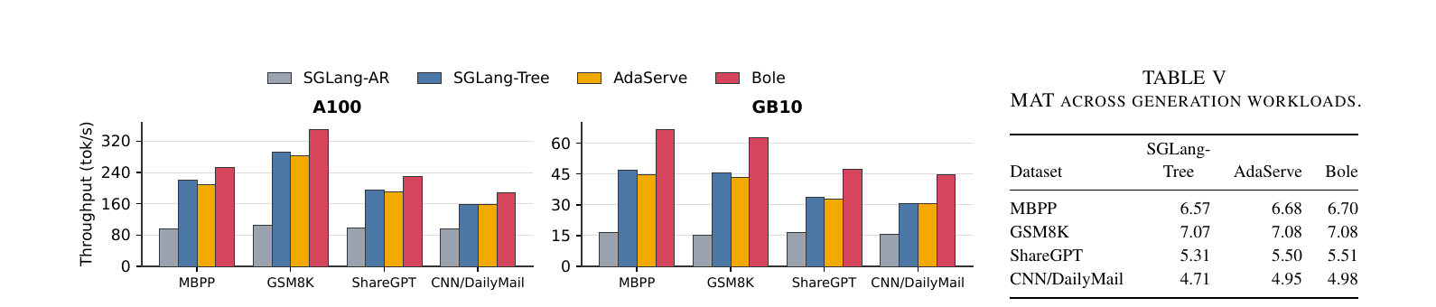
Figure 7 (paper Fig.9): Throughput on four workloads with very different prediction difficulty — code (MBPP), math (GSM8K), dialogue (ShareGPT), summarization (CNN/DailyMail) — at batch size 4. Mean accepted tokens range from 4.98 (CNN/DailyMail, hardest to predict) to 7.08 (GSM8K, most templated/predictable), and Bole’s relative advantage over SGLang-AR (1.98x–3.36x on A100, 2.85x–4.12x on GB10) holds across this entire difficulty spectrum, indicating the gains are not an artifact of one easy workload.

Real-world online agent serving. Replaying multi-turn OpenHands coding-agent sessions (from NVIDIA’s Open-SWE-Traces) under Poisson-process arrivals, Bole reduces mean TTFT (time to first token) by 15.8–64.3% and mean TPOT (time per output token) by 37.6–67.6% versus SGLang-AR; against the strongest speculative baseline (AdaServe), the reductions are 61.3–73.3% (TTFT) and 28.9–49.9% (TPOT). The mechanism behind the TTFT improvement is a subtle but important interaction: because agent sessions repeatedly extend a long shared prefix across turns, evicting a cached prefix (to make room for transient tree-verification state) forces an expensive re-prefill on the next turn. Bole’s factorized state frees enough memory that it attains 90.8%/92.6% prefix-cache hit rates on A100/GB10 — nearly matching plain autoregressive decoding’s 89.8%/93.3% — while SGLang-Tree and AdaServe only reach 58–70% because their state snapshots crowd out cached prefixes. TTFT and TPOT then reinforce each other under continuous batching: lower TPOT frees batch slots sooner (shorter queueing, helping TTFT), and fewer forced re-prefills reduce interference with in-flight decoding (helping TPOT).

Isolating the kernel itself. Comparing just the value-tiled verifier against SGLang-Tree’s serial delta-rule verifier on Qwen3.5-9B (Table VII in the paper), the complete verification core (not just Design 1’s matmuls, but the whole fused Gated-DeltaNet layer) speeds up 3.4x at batch size 1 up to 7.7x at batch size 16, with achieved GPU occupancy rising 3.6x–7.9x and L1/shared-memory throughput rising 1.8x–4.1x. Notably, state materialization alone consumed 38% of serial verification time on A100 but 86% on GB10 for one measured configuration — a striking illustration of how the same algorithmic bottleneck (per-node HBM snapshot writes) can dominate very differently depending on a GPU’s HBM bandwidth relative to its compute throughput.

Component ablation. Cumulatively adding Bole’s three designs to a SGLang-Tree baseline under the online agent workload: the hardware-aware budget alone contributes +5.3% (A100) / +10.7% (GB10) — this step changes nothing about the serial verifier itself, it only stops over-expanding the batch once additional proposals cost more than their expected accepted-token value. Adding the parallel closed-form solver raises the cumulative gain to 1.21x (A100) / 1.30x (GB10) — a bigger jump than budgeting alone, because the selected proposal budget still contains many independent branches whose parent-to-child execution chain the solver removes. Finally, adding factorized state management raises the cumulative speedup to 1.59x (A100) / 2.23x (GB10) — the single largest individual contribution, and disproportionately larger on GB10 due to its tighter memory capacity and larger cache-hit-rate improvement. The ordering of contributions (budget < solver < factorization) is a useful empirical signal about where future hybrid-attention speculative-decoding work should focus first if starting from scratch.

Sensitivity to the verification budget. Sweeping the total verified tree-token budget while holding tree width/depth/batch size fixed (Qwen3.5-9B/MBPP, batch size 8), throughput initially rises with budget (more likely branches get verified, raising MAT faster than cost grows), peaks, then declines once additional verification work outpaces its acceptance benefit. Critically, the peak occurs at a different absolute budget on each platform — 128 total tree tokens on A100, 256 on GB10 — direct empirical confirmation that a single fixed, hardware-agnostic budget (as most existing systems effectively hardcode) cannot be simultaneously optimal across GPUs, validating Design 3’s calibrate-per-configuration approach.

9. Limitations the paper is candid about — and a few it understates

The paper is reasonably forthcoming about some boundary conditions, which is worth crediting: it explicitly notes the maximum-depth $d$ used in the Neumann series (Eq. (6)) is fixed at compile time, that $(b_k, b_v)$ are chosen from a small set of compile-time configurations rather than tuned continuously, and that the offline calibration in Design 3 must be redone whenever the model, GPU, or parallelism setup changes.

Beyond what’s stated directly, a few things are worth flagging that the evaluation doesn’t fully surface:

• The drafter is always the model’s native MTP head. Every experiment uses the same multi-token-prediction drafter shipped with each Qwen3.5 checkpoint. This is a reasonable default, but it sidesteps a question that matters in practice: MTP drafters and separately-trained EAGLE-style drafters have different quality/latency profiles, and it’s unclear whether Bole’s gains (especially the MAT improvements attributed to the utility-maximizing scheduler in Algorithm 3) are robust to a weaker or differently-calibrated drafter, where cumulative path probabilities $\rho(v)$ might be a noisier signal.
• All experiments use unquantized weights. Given that quantization (INT4/INT8 weight-only, or KV-cache quantization) is now standard in production serving, and given that Bole’s whole value proposition is partly about freeing HBM capacity, it would have been useful to see whether the memory savings compound with (or are made partially redundant by) weight/KV quantization — i.e., does Bole’s advantage shrink once you’ve already freed memory another way?
• Only Qwen3.5-family hybrid models are evaluated. Kimi Linear is name-checked in the introduction as another hybrid-attention model but never evaluated. Since Bole’s closed form is derived specifically for the gated delta rule (Eq. (1)), and different hybrid architectures use different recurrent formulations (e.g., different gating structures, different interleaving ratios of full/linear layers), the paper’s claim of general applicability to “hybrid-attention LLMs” is somewhat broader than what’s actually demonstrated — the theorem is specific to gated delta recurrences, and the evaluation is specific to one model family built on that recurrence.
• Tree depth is capped at 8 and top-k at 4 throughout. These are reasonable defaults matching common EAGLE-2-style configurations, but the paper’s own Lemma-3 argument (nilpotency degree bounded by tree depth $d$) implies the parallel solver’s relative advantage should shrink as $d$ grows large (more Neumann rounds, each still parallel across nodes, but more of them). The paper doesn’t report how Bole’s speedup degrades as maximum depth is pushed well beyond 8, which is exactly the regime where the serial-recurrence baseline would also degrade, so the relative comparison at very large depth is left unclear.
• The $\epsilon$ latency-tolerance knob (Eq. (12)) is never swept, as noted in §6 — only the total token budget is swept (Fig. 11). Since $\epsilon$ directly controls the tradeoff between decode-latency overhead and MAT gain, and different serving SLOs (interactive chat vs. batch code review) would plausibly want very different $\epsilon$, this is a meaningful gap for anyone trying to deploy Bole under a specific latency SLO rather than reproduce the paper’s own throughput-oriented benchmarks.

Concrete improvement suggestions

1. Report a depth-sensitivity ablation. Since the theoretical argument for Design 1’s benefit is explicitly depth-dependent (Lemma 3), a plot of speedup-vs-baseline as a function of maximum tree depth $d$ (holding $T$ roughly fixed) would directly validate or bound the paper’s central claim, rather than leaving it implicit in the fixed $d=8$ used throughout.
2. Evaluate at least one non-Qwen hybrid model (Kimi Linear, or a smaller open hybrid model if Kimi Linear weights aren’t practically available) to substantiate the “hybrid-attention LLMs” generality claim, even at reduced scale.
3. Combine with weight/KV quantization in at least one experiment to clarify whether Bole’s memory savings are complementary to or overlapping with the memory savings already achievable via quantization — this is directly relevant to whether a practitioner should expect the reported 2–4x throughput gains to hold in an already-quantized production deployment.
4. Sweep $\epsilon$ explicitly, or at minimum report the range of $\epsilon$ values used across the different reported experiments, so readers deploying under a specific latency SLO have a starting point rather than needing to re-run the offline calibration themselves from scratch.

10. Reproducibility notes

The paper reports an implementation of ≈ 6.2 kLoC of Python and Triton integrated into SGLang release/v0.5.12, which is a substantial, non-trivial engineering artifact; as of this review, no public code release URL is stated in the paper text itself, so reproduction would require re-implementing the closed-form kernel (Algorithm 1/Figure 4 above) and the factorized-state commit path (Algorithm 2) from the paper’s equations, or waiting for/requesting an open-source release from the authors (Nanjing University / Ant Group). The evaluation hardware (4x A100 80GB SXM4, one NVIDIA DGX Spark GB10) is specialized but not exotic; Qwen3.5 model checkpoints from 4B to 122B-A10B parameters are the evaluated targets. Workload datasets (MBPP, GSM8K, ShareGPT, CNN/DailyMail, and Open-SWE-Traces for the online agent evaluation) are all public and standard. The trickiest reproduction step is likely the offline calibration sweep in Design 3 (Eq. (12)), since $B_{\mathrm{ver}}(c)$ is empirically measured per hardware/model/parallelism configuration and is not something you can simply read off from the paper — anyone reproducing this system on different hardware would need to re-run their own calibration sweep rather than reuse the paper’s reported budgets (128 tokens on A100, 256 on GB10 for the specific setting in Fig. 11) directly.

11. Conclusion

Bole is a clean example of taking a production bottleneck seriously enough to actually derive an exact reformulation of the underlying computation, rather than reaching for an approximation. The central insight — that a tree-shaped recurrent dependency structure, once correctly rearranged into a linear system, has a nilpotency degree bounded by tree depth rather than tree size — is genuinely elegant, and it composes well with the second insight that a linear-attention state’s path-factorized representation (Lemma 1) makes exact-but-cheap state management possible without ever materializing a full snapshot per candidate branch. The empirical results (up to 4.72x offline throughput over autoregressive decoding, up to 2.03x over the strongest existing tree-speculative baseline, and up to 67.6%/49.9% TTFT/TPOT reduction under a real agentic workload) are substantial enough to matter for anyone actually deploying hybrid full/linear-attention models like Qwen3.5 or Kimi Linear in production. The honest caveats — evaluation confined to one model family built on one specific recurrence, no quantization interaction studied, and an unswept latency-tolerance knob that matters for SLO-sensitive deployments — don’t undercut the core algorithmic contribution, but they do mean “hybrid-attention LLMs” in the title should currently be read as “models using the gated delta rule,” with generalization to other recurrent formulations (SSMs with different gating, other delta-rule variants) left as a natural next step rather than something this paper has already demonstrated.