QEvict: Recoverable Quantized KV Eviction for Attention-Drift-Robust Long-Context Decoding

Review date: 2026-08-08 Author: Zhongzhu Zhou Paper reviewed: QEvict: Recoverable Quantized KV Eviction for Attention-Drift-Robust Long-Context Decoding Paper authors: Ayushman Garg, Akshita Gupta, Shaswata Bhattacharya, Abhishek Gupta, Sandeep Kumar, Manoj Kumar (IIT Roorkee, IIT Delhi) arXiv: 2608.05326 Venue/Status: Preprint (cs.LG), August 2026

1. The problem: eviction is a one-way door, but importance is not one-way

Every KV-cache compression method for long-context LLM inference has to answer the same question at some point: which tokens get to stay? The dominant answer for the last two years has been eviction — score every cached token or window by how much attention it has received, keep the top-scoring subset, and permanently discard the rest. StreamingLLM keeps sink tokens plus a recent window. H2O keeps “heavy hitters” by accumulated attention mass. SnapKV, AdaKV, CriticalKV, and DefensiveKV progressively refine how the scoring and budget allocation happen — using an observation window, adaptive per-head budgets, value-aware signals, or robustness to future uncertainty, respectively.

All of these methods share a structural assumption that this paper attacks directly: once a token or window is evicted, it is gone, and the implicit bet is that its future relevance is well-predicted by its past relevance. The paper’s core empirical claim is that this bet is worse than it looks. Attention is not just sparse; it drifts. A block of tokens that looks irrelevant at decode step 50 — say, an entity or clause the model has moved past — can become critical at decode step 150 when the model needs to resolve a coreference, retrieve a fact it stated earlier, or pivot its reasoning back to something mentioned much earlier in a long document. Binary eviction cannot represent “I’m not sure I need this anymore, but let me keep a cheap trace of it just in case.” It can only say yes or no, and once it says no, the information is unrecoverable regardless of how the model’s needs evolve.

The competing family of methods — KV-cache quantization (KIVI, KVQuant, ZipCache) — takes the opposite strategy: keep everything, but represent most of it at reduced numerical precision (2–4 bits instead of 16). This preserves broad historical coverage (nothing is thrown away) but pays a different cost: quantization error is applied uniformly or by simple heuristics, without distinguishing “I have strong evidence this region matters” from “I have no idea if this region matters.” At very tight memory budgets, this can waste precision on genuinely unimportant regions while starving genuinely important ones of full-precision fidelity.

QEvict’s proposal is to stop treating “eviction” and “quantization” as two separate compression strategies you must choose between, and instead treat them as two points on a continuum of representation fidelity that a single window can move between dynamically, in both directions, as the model’s actual attention pattern reveals which regions matter right now. A window starts in full precision, can be demoted to a compact INT2 representation when its accumulated attention score drops, can be promoted back to full precision if its score rises again later, and is only permanently evicted once it falls outside both the full-precision and quantized capacity budgets. This turns cache management from a one-shot classification problem into an ongoing routing problem — closer in spirit to a memory hierarchy (L1/L2/disk with demand paging) than to a filter.

Prerequisites: what you need to know before diving in

The KV cache and why it dominates long-context memory. In autoregressive decoding, a transformer caches the key ($K$) and value ($V$) projections for every previously generated token at every layer, so it doesn’t have to recompute them at every new decoding step. For a model with $L$ layers, $H_{kv}$ KV heads, head dimension $d_{kv}$, and sequence length $n$, the cache grows as $O(L \cdot H_{kv} \cdot d_{kv} \cdot n)$ per batch element — linear in sequence length, and for models with large batch sizes and long contexts, this can rival or exceed the memory footprint of the model’s own parameters. This is why “how do we make the KV cache smaller without hurting the model” is one of the most active areas in efficient LLM serving.

Attention-derived importance scoring. Most eviction methods use the attention weights themselves as a signal for which cached states matter. If $a_t^{\ell,h}(i)$ is the softmax attention probability that query token $t$, at layer $\ell$, head $h$, assigns to a cached key $i$, then summing or accumulating these probabilities over many decoding steps gives you an empirical importance score for token/window $i$: tokens that consistently receive high attention are “important,” tokens that never get attended to are candidates for removal. The key subtlety this paper focuses on is that this score is a moving target — it is a function of which queries have been issued so far, and future queries can behave very differently from past ones.

Grouped-Query Attention (GQA) and FlashAttention-2, briefly. GQA reduces KV-cache size by having multiple query heads share a smaller number of KV heads (so $H_{kv} < H_q$), cutting the cache size proportionally. FlashAttention-2 is a fused, IO-aware attention kernel that avoids materializing the full $n \times n$ attention matrix, making both training and inference dramatically faster and more memory-efficient at long context lengths. QEvict is explicitly designed to be compatible with both, though — as we’ll see in the results — the interaction with FlashAttention-2’s fused kernel is one of the paper’s most interesting nuances.

Low-bit KV quantization, briefly. Rather than storing keys and values as 16-bit floats, you can store them as, say, 2-bit or 4-bit integers plus a small number of per-block scale/zero-point parameters, dequantizing back to floating point right before the attention computation. KIVI popularized asymmetric quantization for KV caches — noting that keys and values have different statistical distributions (keys tend to have more structured, per-channel patterns; values are closer to per-token distributions) and should therefore be quantized along different axes. QEvict reuses this same asymmetric per-channel-key / per-token-value scheme, but adds a crucial twist: quantization only ever happens once per window (on its first demotion), and the resulting low-bit representation is cached and reused for every subsequent promotion/demotion cycle, rather than being recomputed from scratch every time.

2. Architecture and pipeline overview

QEvict organizes decoding-time cache management into three stages that repeat throughout generation.

flowchart TB
    subgraph S1["Stage 1: Input & Windowing"]
        A["Input token sequence"] --> B["Partition into contiguous<br/>semantic windows ω1, ω2, ω3, ..."]
        B --> C["All windows initially stored<br/>in full precision (FP16/BF16)"]
    end
    subgraph S2["Stage 2: Cumulative Window Scoring"]
        D["Query at decode step t"] -->|attends to| E["KV Cache"]
        E --> F["Per-window attention score,<br/>accumulated over routing interval Ω"]
        F --> G["Rank windows by cumulative score S̄(w)"]
    end
    subgraph S3["Stage 3: Dynamic Tier Routing"]
        H["Tier 1: Full-Precision Cache<br/>(top Kf windows)"]
        I["Tier 2: Quantized Recoverable<br/>Cache, INT2 (next Kq windows)"]
        J["Tier 3: Permanent Eviction<br/>(remaining windows)"]
        H <-->|Promote/Demote| I
        I -->|Evict, only if outside Kf+Kq| J
    end
    S1 --> S2
    S2 --> S3
    S3 -->|every Ω generated tokens: rescore & reroute| S2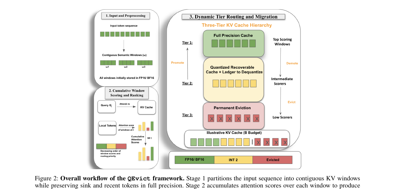

Figure 1 (paper Fig.2): Overall workflow of the QEvict framework. Stage 1 partitions the input sequence into contiguous KV windows while preserving sink and recent tokens in full precision. Stage 2 accumulates attention scores over each window to produce a stable importance ranking. Stage 3 routes windows under a fixed byte budget into a full-precision tier, a recoverable INT2 tier that remains available for attention and later promotion, or permanent eviction, with dynamic promotion and demotion as importance evolves.

Three details matter here beyond the high-level flow. First, windows, not individual tokens, are the routing unit. This is a deliberate design choice discussed below — it stabilizes the ranking against transient per-token attention noise and preserves the local coherence of natural language (entities, clauses, and discourse relations that span several adjacent tokens). Second, routing happens periodically, every $\Omega$ generated tokens, not every step — this amortizes the cost of rescoring across many decode steps. Third, and most important, the arrows between Tier 1 and Tier 2 go both ways: this is the entire point of the paper. A window that gets pushed down to INT2 is not gone; it continues to participate in attention (at reduced precision) and continues accumulating attention score, so if the model’s queries start attending to it again, it gets promoted back to full precision at the next routing event.

3. Diagnosing the problem before proposing the fix

Before presenting the mechanism, the authors run a set of diagnostic experiments on Llama-3.1-8B-Instruct (512-token prefill, 256 generated tokens, 20% KV budget, 5 protected sink tokens) that motivate every design choice in Section 4. This is worth walking through carefully because it’s rare to see a systems paper this explicit about measuring the failure mode before proposing the fix, rather than just proposing a fix and showing it beats baselines.

They define two new diagnostics:

Future Missed Mass (FMM). At decode step $t$, run the uncompressed FullKV model to get the ground-truth attention distribution over the entire cache. FMM measures what fraction of that ground-truth attention mass, at every future decoding step, lands on tokens that a given compressed policy has already permanently discarded by step $t$. Intuitively: if a policy’s FMM is high, it means the compressed model is “flying blind” with respect to information the uncompressed model would actually be using.

Global LIR (Long-term Importance Revival) measures how often a window that has been inactive (not in the full-precision set) for a sustained period later re-enters the full-precision set. A low revival rate would validate the standard eviction assumption (once unimportant, stays unimportant); a non-trivial revival rate would falsify it.

They also define Selection Churn as the Jaccard distance between the sets of retained windows/tokens across consecutive routing events — a measure of how unstable the compressed cache’s notion of “what matters” is from one routing event to the next.

Observation I: windows stabilize cache decisions

Comparing token-level eviction (window size $\Omega_w=1$, called R1) against window-based routing (R3, $\Omega_w=8$; R4, $\Omega_w=32$), Figure 1a shows window-based policies have substantially lower FMM throughout decoding than token-level eviction. Quantitatively, Selection Churn drops from 0.017 for R1 (token-level) to 0.0012 for R3 (window size 8) — over an order of magnitude more stable — and rises again to 0.018 for R4 (window size 32, too coarse). This is the empirical justification for choosing windows over individual tokens as the routing unit: individual-token attention scores are noisy and volatile from one routing event to the next, but the average score over a contiguous span of ~8 tokens is a much more stable signal, without being so coarse (as at window size 32) that you lose fine-grained discrimination between genuinely important and unimportant regions.

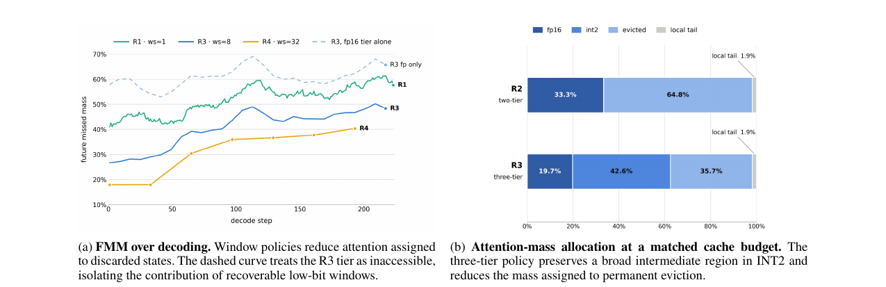
Figure 2 (paper Fig.1): Diagnostics motivating window-level routing and recoverable low-bit retention. (a) Contiguous-window routing reduces Future Missed Mass, while the gap between the solid and dashed R3 curves shows the future utility of the quantized tier. (b) At the same KV-cache budget, three-tier allocation preserves substantially more ground-truth attention mass than binary full-precision retention and eviction.

Observation II: binary eviction throws away a useful middle region

Comparing a two-tier policy (R2: full-precision + eviction only) against the proposed three-tier policy (R3: full-precision + INT2 + eviction) at the same byte budget and window size, Figure 1b shows: R2 retains 33.3% of ground-truth attention mass in full precision and evicts 64.8% (the rest is a small local tail). R3 retains only 19.7% in full precision but preserves an additional 42.6% in the INT2 tier, shrinking the truly evicted share down to 35.7%. Crucially, the INT2 scores computed from the quantized tier maintain 0.9824 cosine agreement with the corresponding FullKV attention scores — meaning the quantized representation is accurate enough to still produce a usable importance signal, not just usable content. And disabling access to the R3 quantized tier (i.e., treating it as if it were evicted, shown as the dashed curve in Figure 1a) makes FMM jump back up close to the R1/R2 level — direct evidence that the windows sitting in the INT2 tier really are being consulted usefully by future decoding steps, not just sitting there uselessly.

Observation III: importance is persistent but not static

This is the observation that most directly justifies the promotion/demotion mechanism. Global LIR is measured two ways: for an oracle top-ranked full-precision set (recomputed with perfect hindsight), the revival rate is only 0.98% — meaning the dominant set of “truly important” windows is mostly stable once you know the ground truth. But for the deployed full-precision policy (making decisions online, without hindsight), the revival rate is 6.18% — over six times higher. In other words: online cache-management decisions are noisier than the underlying ground truth, and a meaningful fraction of windows genuinely do leave and later re-enter the important set. The paper also notes that demotion is substantially more frequent than promotion — importance more often decays than resurges, which is exactly the asymmetry you’d expect and exactly why a recoverable intermediate tier (rather than symmetric eviction) is the right structural response: you want an inexpensive place to park windows during their (usually longer) periods of low apparent importance, from which they can cheaply be pulled back during their (rarer, but real) periods of resurgence.

4. The QEvict mechanism, formalized

4.1 Problem setup

Consider transformer layer $\ell$ with $H_q$ query heads and $H_{kv}$ KV heads (GQA-style, $H_{kv} \le H_q$), head dimension $d_{kv}$. At decoding step $t$, a query $q_t^{\ell,h}$ attends over the currently accessible keys and values:

$$a_t^{\ell,h} = \mathrm{softmax}\left(\frac{q_t^{\ell,h}\left(K_{\mathrm{acc},t}^\ell\right)^\top}{\sqrt{d_{kv}}}\right), \qquad o_t^{\ell,h} = a_t^{\ell,h} V_{\mathrm{acc},t}^\ell. \tag{Attention}$$

This is standard scaled-dot-product attention, with the one nuance that $K_{\mathrm{acc},t}^\ell$ and $V_{\mathrm{acc},t}^\ell$ — the “accessible” keys/values — are reconstructed at every routing/attention step from whatever mixture of full-precision and dequantized-INT2 windows currently exist. Evicted windows contribute nothing; they simply don’t appear in this reconstruction.

After reserving a protected sink prefix $S$ (a handful of always-full-precision anchor tokens, following StreamingLLM’s observation that early tokens act as attention “sinks”) and a protected recent region $L_t$ (the most recently generated tokens, which haven’t yet been scored), the remaining historical cache is partitioned into contiguous windows $\mathcal{W}_t$. Each window $w$ is assigned a state:

$$z_t^\ell(w) \in \{\mathrm{Full}, \mathrm{Quantized}, \mathrm{Evicted}\}. \tag{State}$$

Let $M_f(w)$ and $M_q(w)$ denote the storage cost (in bytes) of window $w$ under full-precision and quantized representation, respectively. The overall assignment across all windows at layer $\ell$ must satisfy a byte budget:

$$B_{\mathrm{sink}} + B_{\mathrm{local}} + \sum_{w \in \mathcal{W}_t} \Big[ \mathbb{1}\!\left[z_t^\ell(w) = \mathrm{Full}\right] M_f(w) + \mathbb{1}\!\left[z_t^\ell(w) = \mathrm{Quantized}\right] M_q(w) \Big] \le B_{\mathrm{total}}. \tag{Budget}$$

The design intuition: $B_{\mathrm{sink}}$ and $B_{\mathrm{local}}$ are fixed overheads (sinks and the recent window are always full precision, by assumption, because they’re small and consistently important). Everything else must fit within what’s left of $B_{\mathrm{total}}$. Note that this formalizes exactly the point made in the introduction: QEvict is jointly deciding residency (is this window kept at all?) and representation precision (if kept, at what bit-width?) — it is not choosing a single retained subset the way pure eviction methods do; it’s choosing a subset-and-precision-assignment jointly.

4.2 Cumulative window scoring — derivation and intuition

Let $a_\tau^{\ell,h}(i)$ be the attention probability assigned to cached token $i$ by query head $h$ at decoding step $\tau$. At a routing event $t$ (occurring every $\Omega$ generated tokens, so $t \equiv 0 \pmod{\Omega}$), the cumulative score of window $w$ is updated incrementally:

$$\overline{S}_t^\ell(w) = \overline{S}_{t-\Omega}^\ell(w) + \frac{1}{H_q}\sum_{h=1}^{H_q}\sum_{\tau=t-\Omega+1}^{t}\sum_{i \in w} a_\tau^{\ell,h}(i), \qquad t \equiv 0 \pmod{\Omega}. \tag{1}$$

Let’s unpack this step by step, because the structure here encodes several design decisions at once:

• The innermost sum, $\sum_{i \in w} a_\tau^{\ell,h}(i)$, aggregates attention probability across all tokens in window $w$, for a single query step $\tau$ and a single head $h$. This is the “windowing” of the score — instead of tracking per-token attention (which Observation I showed is noisy), you get one number per window per step per head.
• The middle sum, over $\tau$ from $t-\Omega+1$ to $t$, accumulates that windowed score across all decode steps since the last routing event. This is what makes the scoring “cumulative” rather than instantaneous — a window that gets briefly high attention on a single step but is otherwise ignored won’t dominate the ranking; a window that gets moderate but consistent attention across the whole interval will.
• The outer sum over $h$, divided by $H_q$, averages across query heads. This is a simplifying design choice: rather than maintaining per-head importance (which would multiply the bookkeeping overhead by $H_q$), QEvict collapses to one score per window per layer. The obvious alternative — per-head routing, as AdaKV does — would in principle allow finer-grained allocation (a window could be important to head 3 but not head 7), but at the cost of $H_q\times$ more routing decisions and metadata to track; QEvict’s ablations (Appendix G, referenced but not reproduced in the main text) find this averaged score sufficient in practice.
• The recurrence $\overline{S}_t = \overline{S}_{t-\Omega} + (\text{new interval's contribution})$ means the score is an additive accumulator across the entire generation history, not a windowed or exponentially-decayed running average. This has a specific implication worth calling out: a window that received a lot of attention early in generation and none since will still have a high cumulative score much later — the score never forgets. This is consistent with Observation III’s finding that important windows are mostly persistent, but it does raise a natural design question (discussed below) about whether very long generations might eventually need some form of decay to let recency dominate over ancient history.

4.3 Byte-constrained tier allocation — derivation

Given the remaining historical budget $B_{\mathrm{hist}} = B_{\mathrm{total}} - B_{\mathrm{sink}} - B_{\mathrm{local}}$ and a chosen quantized-tier fraction $q \in [0,1]$ (a hyperparameter — what fraction of the historical budget goes to the INT2 tier versus full precision), the capacities of the two tiers are:

$$K_f = \left\lfloor \frac{(1-q)B_{\mathrm{hist}}}{M_f} \right\rfloor, \qquad K_q = \left\lfloor \frac{qB_{\mathrm{hist}}}{M_q} \right\rfloor. \tag{3}$$

The derivation here is simple division-and-floor: if you decide the quantized tier gets fraction $q$ of the byte budget, and each quantized window costs $M_q$ bytes, then you can fit $\lfloor qB_{\mathrm{hist}} / M_q \rfloor$ quantized windows; symmetrically for the full-precision tier with the remaining $(1-q)$ fraction. The paper’s ablations (Section 5, briefly summarized in the main text) find $q=0.70$ works well across benchmarks — i.e., roughly 70% of the historical budget goes toward the cheaper INT2 tier, letting it cover far more of the sequence, while the remaining 30% buys full-precision fidelity for the highest-scoring windows. This asymmetry makes sense given Observation II: the quantized tier is what lets you preserve broad coverage under a tight budget, while the full-precision tier is reserved for the windows you’re most confident matter right now.

4.4 Dynamic routing and recovery — the promotion/demotion algorithm

At each routing event, the pool of candidate windows for the full-precision and quantized tiers is:

$$\mathcal{W}_t^{\mathrm{cand}} = \mathcal{F}_{t-\Omega} \cup \mathcal{Q}_{t-\Omega} \cup \mathcal{L}_t^{\mathrm{aged}}. \tag{4}$$

This says: the candidates are whatever was in the full-precision tier last routing event, whatever was in the quantized tier last routing event, plus any windows that have just “aged out” of the protected recent region $\mathcal{L}_t$ and are now eligible to be ranked and routed for the first time. Candidates are then ranked by their cumulative score $\overline{S}_t^\ell(w)$ from equation (1), and assigned greedily from the top:

$$\mathcal{F}_t = \mathrm{TopK}_{K_f}\!\left(\mathcal{W}_t^{\mathrm{cand}}; \overline{S}_t^\ell\right),$$ $$\mathcal{Q}_t = \mathrm{TopK}_{K_q}\!\left(\mathcal{W}_t^{\mathrm{cand}} \setminus \mathcal{F}_t; \overline{S}_t^\ell\right), \tag{5}$$ $$\mathcal{E}_t = \mathcal{W}_t^{\mathrm{cand}} \setminus (\mathcal{F}_t \cup \mathcal{Q}_t).$$

In words: take the $K_f$ highest-scoring candidates into the full-precision tier; of what remains, take the next $K_q$ highest-scoring candidates into the quantized tier; whatever’s left over is evicted. Because quantized windows remain available to attention and continue accumulating score (equation 1 doesn’t distinguish where a window currently lives — it just accumulates attention received, and a quantized window still participates in attention, just at reduced precision), a window’s fate is genuinely reversible across routing events:

$$\mathrm{Full} \rightleftarrows \mathrm{Quantized} \longrightarrow \mathrm{Evicted}. \tag{6}$$

Only windows that fall outside the combined capacities $K_f + K_q$ — i.e., windows that don’t even make the cut for the cheap quantized tier — are permanently removed. This is the crux of the whole mechanism: eviction is now a last resort applied only to the truly lowest-ranked candidates, not a binary fate applied to everything below a single threshold.

Algorithm 1 (Dynamic Tier Routing at Routing Event $t$)

Input: cumulative scores S̄_t(w) for all candidate windows w ∈ W_cand,
       capacities K_f (full-precision) and K_q (quantized),
       previous tier assignment (F_{t-Ω}, Q_{t-Ω})
Output: new tier assignment (F_t, Q_t, E_t)

1.  W_cand ← F_{t-Ω} ∪ Q_{t-Ω} ∪ L_aged           // build candidate pool (Eq. 4)
2.  for each window w in W_cand:
3.      compute S̄_t(w) via Eq. (1)                // accumulate attention since last routing event
4.  sort W_cand in descending order of S̄_t(w)
5.  F_t ← top K_f windows from sorted W_cand        // promote/retain in full precision
6.  remaining ← W_cand \ F_t
7.  Q_t ← top K_q windows from sorted remaining     // demote/retain in quantized tier
8.  E_t ← remaining \ Q_t                           // permanently evict the rest
9.  for each window w in Q_t:
10.     if w was NOT previously quantized (w ∉ Q_{t-Ω}):
11.         quantize w using asymmetric per-channel-key / per-token-value scheme
12.         store quantization codes + scale/zero-point in persistent ledger
13.     else:
14.         reuse existing quantization codes from ledger  // migration-stable, no re-quantization
15. for each window w in F_t:
16.     if w was previously in Q_{t-Ω} (i.e., being promoted):
17.         dequantize w using stored codes from ledger
18.         re-apply RoPE at w's original absolute positions
19. return (F_t, Q_t, E_t)

Two implementation details in this pseudocode deserve derivation-level attention because they’re what prevents the recoverable tier from degrading over time.

Migration-stable quantization (lines 9–14). The naive way to implement promotion/demotion would be: whenever a window is demoted, quantize it fresh from its current full-precision values; whenever it’s promoted, dequantize; whenever it’s demoted again, quantize again from the (already lossy) dequantized values. This compounds quantization error across repeated migrations — every round-trip through the lossy channel adds more error, the same way repeatedly saving a JPEG degrades it further each time. QEvict’s fix is to quantize a window only on its first demotion ever, store the resulting low-bit codes and quantization parameters (scale, zero-point) in a persistent ledger, and on every subsequent demotion, simply reuse those exact same stored codes rather than re-quantizing from a potentially-already-degraded reconstruction. This means quantization error is incurred exactly once per window, no matter how many times it oscillates between tiers afterward.

Positional handling for promoted keys (lines 15–19). Keys are quantized in the pre-RoPE domain — i.e., before rotary position embeddings are applied — together with their original absolute token positions. When a window is promoted back to full precision, RoPE is reapplied using those stored original positions. Why pre-RoPE? Because RoPE rotates the key vector by an angle depending on its absolute position; if you quantized a key after RoPE was applied, the rotation angle would be baked into the quantized values, and dequantizing later would need to “undo” a rotation from lossy, low-bit-precision data — compounding error in a subtler way. Quantizing before rotation and reapplying the (numerically exact) rotation after dequantization keeps the positional information decoupled from the lossy compression step.

4.5 A worked numerical example

Equations are easier to trust once you’ve pushed real numbers through them. Consider Llama-3.1-8B-Instruct’s KV-cache geometry: $H_{kv}=8$ KV heads (GQA-reduced from 32 query heads), head dimension $d_{kv}=128$, and $L=32$ layers. In BF16 (2 bytes/element), the per-token, per-layer KV footprint is $2 \times H_{kv} \times d_{kv} \times 2\,\text{bytes} = 2 \times 8 \times 128 \times 2 = 4096$ bytes (the leading 2 accounts for storing both $K$ and $V$). Across all 32 layers, that’s $4096 \times 32 = 131072$ bytes $\approx 128\,\text{KB}$ per token in full precision.

Suppose a routing event considers a window of $\omega=8$ tokens. Then $M_f(w) = 8 \times 128\,\text{KB} = 1024\,\text{KB} = 1\,\text{MB}$ per window (summed across all layers, since the byte budget in equation (Budget) is a whole-cache constraint). Quantizing to INT2 (plus a small per-block scale/zero-point overhead, say ~5% metadata) reduces this to roughly $M_q(w) \approx 1\,\text{MB} \times \tfrac{2}{16} \times 1.05 \approx 131\,\text{KB}$ — a compression ratio just under 8x per window, consistent with the paper’s headline claim of INT2 quantization being roughly 8x cheaper than full-precision BF16.

Now plug into equation (3). Suppose the historical budget after reserving sinks and the recent window is $B_{\mathrm{hist}} = 100\,\text{MB}$ (this is a stand-in figure to illustrate proportions, not the paper’s actual RULER 32K configuration) and $q=0.70$ as the paper recommends. Then:

$$K_f = \left\lfloor \frac{0.30 \times 100\,\text{MB}}{1\,\text{MB}} \right\rfloor = 30 \text{ windows} = 240 \text{ tokens (full precision)},$$ $$K_q = \left\lfloor \frac{0.70 \times 100\,\text{MB}}{0.131\,\text{MB}} \right\rfloor \approx 534 \text{ windows} \approx 4272 \text{ tokens (INT2)}.$$

So for the same 100 MB budget that would only buy 240 tokens of coverage under a full-precision-only policy, QEvict’s three-tier split buys 240 tokens of full-precision coverage plus 4272 tokens of INT2-recoverable coverage — roughly 18.8x more total token coverage at the same byte cost, at the price of accepting quantization noise on the larger tier. This concretely illustrates why Observation II’s finding (three-tier retains 62.3% combined attention mass vs. two-tier’s 33.3%) is not surprising once you see the raw arithmetic: the quantized tier is simply so much cheaper per token that even a modest byte allocation buys enormous additional coverage.

5. Design choices: why this way, what’s the alternative, where does it break

Why windows instead of tokens? Why it works: Observation I showed windowing reduces Selection Churn by over 10x (0.017 → 0.0012 at $\Omega_w=8$) while lowering FMM, because natural-language importance is genuinely spatially correlated (a whole clause or entity mention matters or doesn’t, not individual sub-word tokens independently). The obvious alternative: per-token routing (as in the R1 baseline, or conceptually similar to SnapKV/AdaKV’s finer-grained token selection), which gives maximal flexibility to keep exactly the tokens that matter. Where windowing fails: if a window boundary happens to split a genuinely important token from genuinely unimportant neighbors, the whole window gets promoted/demoted based on the noisier neighbors — and Observation I already shows this failure mode at $\Omega_w=32$ (R4), where the FMM curve is much lower on average (fewer things evicted) but this comes at the cost of coarser allocation, wasting budget on unimportant tokens that happen to share a window with important ones. The paper picks $\Omega_w=8$ based on ablation, but this is clearly a dataset/task-dependent sweet spot, not a universal constant, and the paper is honest that this is future work (“adaptive window boundaries… for future study”).

Why a persistent quantization ledger instead of re-quantizing on every demotion? Why it works: it caps total quantization error per window at one round-trip, regardless of how many oscillations occur — verified indirectly by the 0.9824 cosine agreement between INT2 and FullKV scores holding up even under the churn levels reported. The obvious alternative: stateless quantize-on-demand, which is simpler to implement and doesn’t require maintaining an extra data structure (the ledger) alongside the KV cache itself. Where the ledger approach has a cost: memory. The ledger itself has to be stored somewhere, and for workloads with very high churn (many windows oscillating rapidly), the ledger’s own footprint could become non-trivial — the paper doesn’t report ledger memory overhead explicitly, which is a gap worth flagging (see Section 8).

Why $q=0.70$ (70% of the historical budget to the quantized tier)? Why it works: the paper’s own diagnostic (Observation II) shows the quantized tier is where most of the “recoverable coverage” benefit comes from — 42.6 percentage points of attention mass moved from “evicted” to “quantized” at the R2→R3 transition, versus only giving up 13.6 points of full-precision coverage (33.3% → 19.7%). A generous quantized-tier allocation directly targets this asymmetry. The obvious alternative: a more conservative split (e.g., $q=0.3$ or $q=0.5$) that keeps more windows at full precision, sacrificing coverage for higher per-window fidelity on a smaller set. Where $q=0.70$ might not be optimal: for tasks that are extremely sensitive to precision on a small set of critical facts (rather than broad coverage) — e.g., needle-in-a-haystack tasks with a single needle rather than the multi-key/multi-value RULER variants — a smaller $q$ that guarantees more of the sequence stays at full precision might actually do better, and indeed Table 2 shows QEvict’s advantage over baselines is somewhat smaller on the hardest single/multi-key retrieval subtasks (MK-3: QEvict 77.80 vs. DefensiveKV 97.00) than on aggregate/tracking tasks — suggesting the fixed $q=0.70$ isn’t universally optimal across task types.

Why cumulative (never-decaying) scores rather than an exponential moving average? Why it works: Observation III shows the oracle set of important windows is highly persistent (0.98% revival rate) — meaning what matters early tends to keep mattering, so an additive accumulator that never forgets is a reasonable model of ground truth. The obvious alternative: an exponentially-decayed running score that weights recent attention more heavily, which would make the cache more responsive to shifts in topic within a single long generation. Where cumulative scoring could fail: extremely long generations with genuine topic shifts (e.g., a 50K-token document where the model spends the first 10K tokens on one sub-topic and the last 40K on an unrelated one) could see early, no-longer-relevant windows keep an artificially inflated score purely from historical accumulation, crowding out genuinely currently-relevant windows that just haven’t had time to accumulate comparable scores yet. The paper’s own evaluation setups (512-token prefill + 256 generated tokens for diagnostics; up to 32K context for RULER) are within a range where this decay-vs-no-decay question doesn’t obviously bite, but it’s a real open question for the “up to 10M context” regime that adjacent quantization papers (KVQuant) target.

6. Experimental results, reproduced and interpreted

6.1 Long-range retrieval: RULER at 32K context

Table 2 (paper Table 2) reports RULER performance at 32K context on Llama-3.1-8B-Instruct, comparing QEvict against eviction baselines matched at a 20% cache budget and quantization baselines at comparable memory footprints.

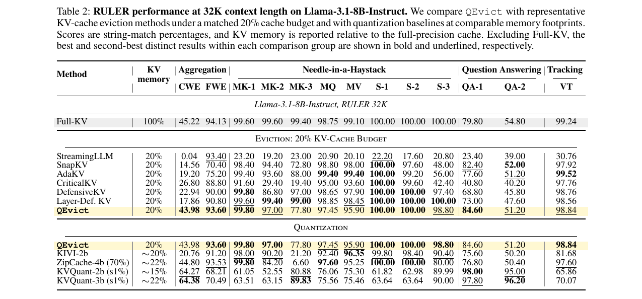
Figure 3 (paper Table 2, reproduced as image): RULER performance at 32K context length on Llama-3.1-8B-Instruct. QEvict achieves the best matched-memory macro-average among both eviction and quantization baseline families.

Reading this table carefully: QEvict achieves a macro-average of 87.6 across the 13 RULER subtasks (aggregation, needle-in-a-haystack variants, QA, and tracking), beating the strongest matched-memory eviction baseline, Layer-DefensiveKV, by 1.2 points, and beating the strongest comparable-memory quantization baseline (KVQuant-3b) by 8.6 points — while staying within 2.4 points of the uncompressed Full-KV reference (which uses 5x the memory). The most striking single number is CWE (Common Word Extraction, an aggregation task): QEvict scores 43.98 versus the best eviction baseline’s 26.80 (CriticalKV) — a >17-point gap. This makes sense given the mechanism: aggregation tasks require synthesizing information scattered non-locally across the context, which is exactly the scenario where “a window I thought was unimportant 10K tokens ago turns out to matter for this specific aggregation query” would bite hardest under permanent eviction. Conversely, on MK-3 (a harder multi-key retrieval variant), QEvict’s 77.80 trails DefensiveKV’s 97.00 — a case where the quantization noise in the INT2 tier apparently does cost some precision on a task that needs exact key matching, consistent with the design-choice discussion above about $q$ possibly being sub-optimal for single-needle-style precision-critical tasks.

6.2 Long-context understanding: LongBench across three budgets

Table 3 (paper Table 3, reproduced as image) reports LongBench performance on Llama-3.1-8B-Instruct and Mistral-7B-Instruct-v0.2, across 12 tasks spanning single-doc QA, multi-doc QA, summarization, and few-shot learning, at 20%, 10%, and 5% KV-memory budgets.

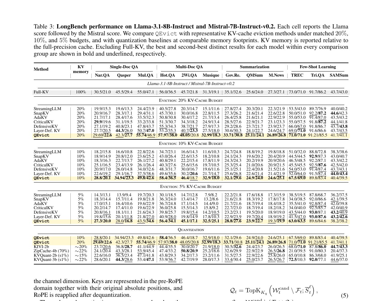
Figure 4 (paper Table 3, reproduced as image): LongBench performance across three KV-cache budgets and two models. QEvict’s advantage over matched-memory baselines widens as the budget tightens.

The pattern worth highlighting is how the gap changes with tightening budget. At 20% memory, QEvict scores 46.4 (Llama) / 37.8 (Mistral) macro-average, versus 44.0 / 37.4 for the strongest eviction baseline — a modest ~2-point edge. But at 5% memory, the gap widens to 9.7 points on Llama and 4.7 on Mistral. This is exactly what the recoverable-tier hypothesis predicts: when there’s enough budget for everyone to keep a reasonably large full-precision set, permanent eviction’s mistakes matter less (there’s more slack to absorb a wrong call). At very tight budgets, every eviction decision is high-stakes, and this is precisely where having a cheap “maybe” tier — rather than forcing every window into a hard yes/no — pays off most. This budget-dependent widening gap is, in my view, the single most convincing piece of evidence in the paper for the core thesis.

6.3 Reasoning under compression: GSM8K

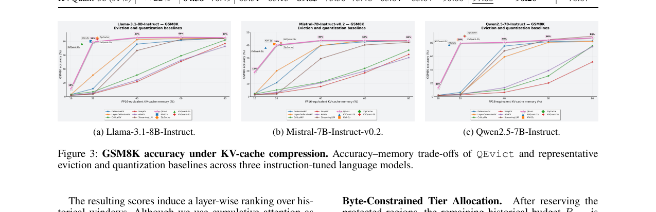
Figure 5 (paper Fig.3): GSM8K accuracy under KV-cache compression. Accuracy–memory trade-offs of QEvict and representative eviction and quantization baselines across three instruction-tuned language models (Llama-3.1-8B-Instruct, Mistral-7B-Instruct-v0.2, Qwen2.5-7B-Instruct).

GSM8K is a useful complementary benchmark to LongBench/RULER because it tests multi-step autoregressive generation quality rather than a single retrieval/comprehension answer — the cache has to stay useful across many self-generated reasoning steps, not just for one final answer extraction. The accuracy-vs-memory curves show QEvict (highlighted line in each panel) tracking close to the top of the Pareto frontier across all three models at low-to-moderate memory budgets, with a particularly pronounced advantage in the 10-20% memory-budget regime — consistent with the mechanism’s core claim: multi-step reasoning is exactly the setting where the model may need to “look back” at intermediate reasoning it generated many steps ago (to check consistency, avoid contradiction, or retrieve an earlier sub-result), which is the scenario permanent eviction handles worst.

6.4 End-to-end serving efficiency: the backend-dependent trade-off

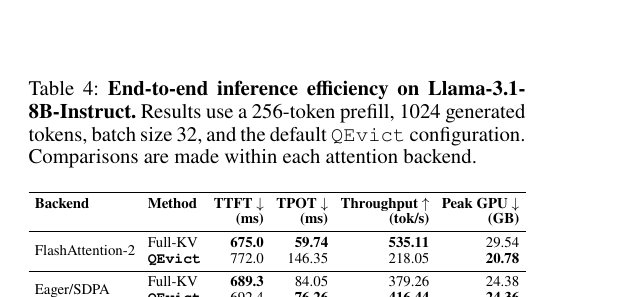
Figure 6 (paper Table 4, reproduced as image): End-to-end inference efficiency on Llama-3.1-8B-Instruct, 256-token prefill, 1024 generated tokens, batch size 32.

This table is the most important one for anyone thinking about actually deploying this, and it’s also where the paper is most honest about a real limitation. Two attention backends give opposite verdicts:

With eager/SDPA attention, QEvict adds only 0.5% time-to-first-token (TTFT) overhead (689.3ms → 692.4ms), reduces per-token latency (TPOT) by 9.3% (84.05ms → 76.26ms), and improves decoding throughput by 9.8% (379.26 → 416.44 tok/s) — a clean, strict win. This makes sense: with a smaller effective attended cache (much of it INT2, some evicted), the raw compute and memory-bandwidth cost of the attention operation itself goes down, and in the eager/SDPA path, this saving outweighs the bookkeeping overhead of dequantization and routing.

With FlashAttention-2, the story flips: TTFT overhead grows to 14.4% (675.0ms → 772.0ms), TPOT gets worse by 145% (59.74ms → 146.35ms), and decoding throughput drops by 59% (535.11 → 218.05 tok/s) — even though peak GPU memory drops by a real 29.7% (29.54GB → 20.78GB). The reason, as the paper is upfront about in its limitations section, is architectural: FlashAttention-2’s speed comes precisely from never materializing the full attention-probability matrix — but QEvict’s routing mechanism needs those attention probabilities to compute the cumulative window scores in equation (1). So at every routing event, QEvict has to fall back from FlashAttention-2 to the slower SDPA path just to expose the attention weights it needs for scoring, plus reconstruct (dequantize, re-apply RoPE) the active low-bit windows before every attention call. In the unfused eager path, this extra work is comparatively cheap relative to the savings; in the fused FlashAttention-2 path, that extra unfused work becomes the dominant cost, more than offsetting the memory savings.

This is a genuinely important nuance that’s easy to miss if you only read the headline throughput numbers: QEvict’s current implementation trades memory for a backend-dependent latency cost, and realizing memory savings and the FlashAttention-2 speed advantage simultaneously would require fused low-bit attention and routing kernels that don’t yet exist for this method — which the paper correctly flags as future work rather than claiming to have solved.

7. Limitations (as stated, and as I see them)

The paper’s own stated limitations (Section 5.1): the current implementation reconstructs active low-bit windows before attention (rather than computing attention directly on quantized representations) and selectively falls back to SDPA at routing events, both of which introduce overhead that a fused kernel implementation could eliminate. The evaluation also focuses on decoder-only models with fixed-size contiguous windows, leaving adaptive window boundaries and other architectures (e.g., encoder-decoder, or architectures beyond standard GQA transformers) for future work.

8. Critical analysis

Weaknesses and flaws specific to this paper. First, the FlashAttention-2 throughput regression (59% decoding-throughput drop, Table 4) is a serious practical caveat that could easily be missed by a reader who stops at the LongBench/RULER accuracy tables — a system that halves your throughput to save 30% memory is not a free lunch for latency-sensitive serving, and the paper would benefit from foregrounding this trade-off earlier and more prominently rather than positioning it as a “limitation” mentioned briefly near the end. Second, the persistent quantization ledger’s own memory overhead is never quantified. Every window that has ever been demoted keeps its quantized codes and quantization parameters resident (to enable cheap re-promotion), but the paper never reports what fraction of the total memory budget the ledger itself consumes, especially under high-churn workloads where many windows cycle repeatedly — this is exactly the kind of “hidden cost” that could erode the headline memory savings in adversarial or long-running conditions. Third, the ablation over routing interval $\Omega$ and quantized-tier fraction $q$ is relegated to an appendix not reproduced in the main text, and the main paper reports only the single “best” configuration ($\Omega=8$, $q=0.70$) across benchmarks — but Section 6’s own results (MK-3 retrieval underperforming, and the budget-dependent gap-widening in LongBench) suggest these hyperparameters are not uniformly optimal across task types, and a reader can’t easily assess sensitivity without digging into the appendix.

Limitations the authors understate or omit. The evaluation is restricted to 7-8B parameter models. Whether the promotion/demotion dynamics, the choice of $\Omega=8$ windowing, and the $q=0.70$ split generalize to much larger models (70B+) with different attention head counts, or to mixture-of-experts architectures where attention patterns per expert-routing decision could behave quite differently, is completely untested. Separately, the routing interval $\Omega$ introduces a real latency-vs-freshness trade-off that isn’t explicitly analyzed: routing every 8 tokens means importance signals can be up to 8 tokens stale at any given moment, and for extremely rapid topic shifts within a generation (adversarial or otherwise), this staleness window could matter more than the paper’s ablations (evaluated only on relatively steady-state long-document tasks) reveal. Finally, the paper never discusses multi-request/multi-tenant serving scenarios (batch size 32 in Table 4 is a single workload replicated, not concurrent heterogeneous requests) — real production serving involves requests at wildly different context lengths and generation stages sharing GPU resources, and it’s unclear how QEvict’s per-request routing overhead composes across a genuinely heterogeneous batch.

Concrete, specific improvement suggestions. (1) Report ledger memory overhead explicitly as a function of churn rate, ideally with a worst-case adversarial workload designed to maximize oscillation between tiers, so practitioners can budget for it rather than discovering it empirically in production. (2) Investigate a hybrid attention-backend strategy — e.g., default to FlashAttention-2 for the bulk of decoding and only fall back to SDPA at the (infrequent, every-$\Omega$-tokens) routing events themselves, rather than implying the fallback affects the whole interval — the paper’s description suggests SDPA is used “at routing events,” but Table 4’s throughput numbers suggest the overhead is much larger than what a brief per-$\Omega$-step fallback alone would predict, and clarifying exactly where the FlashAttention-2 slowdown is concentrated (routing-event steps only, versus every decode step due to dequantization) would make the trade-off analysis much more actionable. (3) Extend the ablation grid (currently $\Omega \in \{1,8,32\}$ and a small set of $q$ values) into a proper sensitivity heatmap over $(\Omega, q)$ jointly, and report per-task-type breakdowns (retrieval-heavy vs. aggregation-heavy vs. reasoning-heavy) rather than only macro-averages, since Section 6 already shows the method’s advantage varies substantially by task type. (4) Test at least one model in the 30-70B range and, if feasible, one MoE architecture, to establish whether the core findings (window-based scoring stability, three-tier recoverability) are model-scale-invariant or specific to the 7-8B regime studied.

8b. Why the accumulator design matters for correctness, not just performance

It’s worth dwelling a moment longer on a subtlety in equation (1) that’s easy to read past: the recurrence $\overline{S}_t^\ell(w) = \overline{S}_{t-\Omega}^\ell(w) + (\text{new contribution})$ is only well-defined if a window’s identity is preserved across routing events — i.e., the system needs to know that “window 47” at routing event $t$ is the same logical span of tokens as “window 47” at routing event $t-\Omega$, even though its physical storage location and representation (full-precision vs. INT2) may have changed in between. This means QEvict’s implementation necessarily maintains a stable window-to-position mapping independent of tier assignment — a bookkeeping requirement that’s implicit in the math but has real engineering weight: every promotion or demotion has to update tier membership without disturbing the identity used to accumulate scores. Contrast this with a hypothetical stateless redesign where scores were recomputed from scratch at each routing event using only the current window’s attention during the current $\Omega$-token interval (i.e., dropping the $\overline{S}_{t-\Omega}^\ell(w)$ term entirely) — this would be simpler to implement (no persistent per-window score state needed) but would throw away exactly the historical signal that Observation III shows matters: a window that was important 200 tokens ago but quiet for the last 8 tokens would score as if it had never mattered, defeating the entire motivation for a persistent, cumulative notion of importance. The paper doesn’t frame it this way explicitly, but the accumulator’s design is inseparable from the diagnostic findings in Section 3 — it is the direct mathematical encoding of “importance is persistent but not static.”

9. Reproducibility notes

The paper reports concrete, checkable hyperparameters: routing interval $\Omega=8$, five protected sink tokens, 32-token protected recent region, INT2 quantized tier, quantized-tier fraction $q=0.70$, evaluated across LongBench, RULER (32K context), and GSM8K on three widely available instruction-tuned open models (Llama-3.1-8B-Instruct, Qwen2.5-7B-Instruct, Mistral-7B-Instruct-v0.2). All three benchmarks are public and standard in the KV-cache-compression literature, which makes independent re-implementation and comparison feasible in principle. The paper states that complete baseline configurations, decoding protocols, and byte-level memory accounting are in the appendices (referenced as Appendix B, G, H, I, J in the main text) — a reader attempting to reproduce results precisely would need those appendices for exact baseline hyperparameters and the precise byte-accounting formula used to compute “matched memory budgets” across such structurally different methods (windows-plus-quantization vs. pure token eviction vs. pure quantization). No code or artifact release is mentioned in the excerpted main text; independent reproduction would require re-implementing the routing algorithm, the migration-stable quantization ledger, and the diagnostic metrics (FMM, Global LIR, Selection Churn) from the equations given.

10. Where this sits in the broader KV-cache-compression landscape

QEvict is best understood as a genuine third category alongside pure eviction (StreamingLLM, H2O, SnapKV, AdaKV, CriticalKV, DefensiveKV) and pure quantization (KIVI, KVQuant, ZipCache): a hybrid, dynamic hierarchy that borrows the “keep the important stuff” instinct of eviction and the “keep everything, just cheaper” instinct of quantization, and resolves the tension between them with a genuinely reversible middle tier rather than picking one philosophy. It shares DNA with classical memory-hierarchy design (the promote/demote/evict structure is directly analogous to a CPU cache hierarchy with an intermediate tier, or to OS-level demand paging with a “recently used but not resident” list) more than with prior KV-cache-specific work, which is a useful lens for thinking about where the idea could go next — e.g., could a fourth tier (disk-backed, as in Tutti’s SSD-backed KV cache) extend this hierarchy further for even longer contexts, with QEvict’s INT2 tier becoming the “L2” between a full-precision “L1” and an SSD-backed “L3”? The paper doesn’t explore this, but the structural fit seems natural.

10b. Comparing QEvict’s design axes against its closest relatives

Table 1 in the paper itself makes a qualitative comparison (selective eviction / low-bit retention / window routing / dynamic recovery), but it’s worth walking through what each competing method actually gives up to make its design simpler, since that’s the real story behind why QEvict’s combination of features is non-trivial rather than an obvious union of prior ideas.

StreamingLLM keeps it deliberately simple: a handful of sink tokens plus a sliding recent window, no scoring mechanism at all. This is essentially free computationally, but it has zero mechanism for keeping any historically important-but-not-recent content, which is why its RULER and LongBench numbers in Tables 2–3 are the weakest across almost every task — it isn’t even trying to solve the problem QEvict targets, it’s solving a cheaper, more restricted problem (bounded-memory streaming) that happens to be evaluated on the same benchmarks.

SnapKV / AdaKV / CriticalKV all improve how importance is scored (observation-window-based, per-head-budget-adaptive, value-aware respectively) but keep the eviction decision binary and permanent — they’re all trying to make the one-shot decision smarter, not to make the decision reversible. QEvict’s contribution is orthogonal to theirs: you could in principle swap QEvict’s cumulative-attention scorer for AdaKV’s adaptive per-head budgeting within QEvict’s three-tier hierarchy, since the routing mechanism (Algorithm 1) only needs some scalar importance signal per window, not specifically the one QEvict uses. The paper doesn’t explore this hybridization, which strikes me as a fairly natural next experiment.

DefensiveKV / Layer-DefensiveKV explicitly model uncertainty about future attention (robustness to distributional shift in what gets attended to later) — conceptually the closest prior work to QEvict’s motivation, since both are reacting to the same underlying problem (importance changes over time). The difference is mechanism: DefensiveKV tries to make the single eviction decision more robust to future drift by hedging at decision time, while QEvict sidesteps the need for robust one-shot decisions entirely by allowing the decision to be revisited. Table 2’s RULER results show these are competitive on different subtasks (Layer-DefensiveKV wins some needle-in-a-haystack variants, QEvict wins aggregation and tracking), suggesting the two philosophies—robust prediction vs. reversible decision—are not strictly dominated by one another and might even compose.

KIVI / KVQuant / ZipCache solve a different problem well: preserving broad coverage cheaply. Their weakness, from QEvict’s perspective, is uniform or coarse-grained precision allocation — they don’t distinguish “I’m confident this matters” from “I have no signal either way,” so at very tight budgets they can’t concentrate precision where it’s needed most. QEvict essentially imports their quantization machinery (the asymmetric per-channel-key/per-token-value scheme is directly inherited from KIVI) but wraps it inside an importance-aware allocation policy, which is why Table 2’s quantization comparison group shows QEvict beating KVQuant-3b by 8.6 points using less memory (20% vs. ~22%) — the win isn’t from a better quantization codec, it’s from spending the same quantization budget more selectively.

Seen this way, QEvict isn’t proposing a new scoring function or a new quantization codec — both of those are borrowed from prior work. Its actual novel contribution is the routing policy that sits between them: the recoverable three-tier hierarchy and the migration-stable ledger that makes revisiting decisions cheap. That’s a fair characterization to make explicit, since a reader skimming only the results tables might assume the gains come from a better scorer or a better quantizer, when they primarily come from architecture-level orchestration of existing techniques.

11. Conclusion

QEvict makes a simple but under-examined point rigorous: the standard assumption behind KV-cache eviction — that once a token looks unimportant, it will stay unimportant — is measurably false often enough to matter, especially for aggregation-style long-context tasks and multi-step reasoning. Its fix, a three-tier recoverable hierarchy with migration-stable quantization, delivers consistent accuracy-per-byte improvements over both eviction and quantization baselines, most visibly at the tightest memory budgets where every eviction decision carries the highest stakes. The mechanism is elegant and the diagnostic groundwork (FMM, Global LIR, Selection Churn) is a genuinely useful contribution independent of the specific algorithm — future KV-cache-compression papers could benefit from reporting these same diagnostics as a matter of course. The main open question, which the paper is refreshingly candid about, is whether the current unfused implementation’s backend-dependent trade-off (a clean win under eager/SDPA, a real throughput regression under FlashAttention-2) can be closed with fused kernels — until then, whether QEvict is a good fit for a given deployment depends heavily on which attention backend that deployment is already committed to.