SALT: Subspace-Aligned Centroid-Residual Training for Efficient Ultra-LoRA Serving

Review date: 2026-08-07 Author: Zhongzhu Zhou Paper reviewed: Pin Once, Swap Light: Subspace-Aligned Centroid-Residual Training for Efficient Ultra-LoRA Serving Paper authors: Xiang Li, Pengcheng Wang, Huazheng Wang, Saurabh Bagchi (Purdue University, Oregon State University) arXiv: 2608.03579 Venue/Status: Preprint (cs.LG), August 2026

1. Why this paper, and what problem is it actually solving

Picture an LLM-as-a-Service platform hosting hundreds of tenant-specific LoRA adapters on top of one shared base model — a coding assistant fine-tuned for one customer, a math tutor fine-tuned for another, a legal-document summarizer for a third. Every incoming request needs its tenant’s adapter loaded before the forward pass runs. The serving engine (say, vLLM with Punica-style batched heterogeneous-adapter kernels) can’t afford to permanently pin every tenant’s weights in GPU VRAM — with hundreds of tenants, that alone would starve the KV cache the model needs to actually serve requests. So it swaps: keep a working set of adapters resident, page others in over PCIe as requests arrive that need them. This is exactly the operational pattern behind “LoRA-as-a-Service” offerings on Amazon Bedrock and similar platforms.

Here is the tension the paper opens with, and it is genuinely a hard trade-off, not a solved problem: adapter rank controls both how much task-specific capacity a tenant gets and how expensive that tenant is to serve. A rank-16 LoRA adapter for a 7B model might need to swap in ~13.6 MB every time it’s needed; that’s real PCIe bandwidth and real latency, multiplied by however many concurrent tenants are cycling through the cache. Drop the rank down to r=1 or r=2 to make swapping cheap, and — unsurprisingly — task accuracy degrades, sometimes badly. Standard LoRA at r=1 on Mistral-7B loses ground on SPIDER (semantic-parsing/text-to-SQL) versus r=16: 30.34% vs 21.34% is actually inverted in the paper’s own table (r=1 slightly beats r=16 there due to noise), but the broader pattern across tasks is real rank-sensitivity and volatility — the paper documents LoRA dropping to 3.00% accuracy on MBPP at r=8 despite scoring 25.50% at r=4, a genuinely unstable relationship between rank and downstream quality that a provider cannot plan capacity around.

Prior attempts to resolve this dilemma fall into two camps, and the paper is specific about why each falls short for real multi-tenant deployment:

Post-hoc compression (“Compress then Serve,” joint diagonalization across many pre-trained adapters to extract a shared basis) requires the adapters to already exist at high rank before you can compress them — so you pay the original serving cost during onboarding — and worse, it needs access to every tenant’s private adapter weights simultaneously to compute the shared basis, which is a real data-isolation problem in a multi-tenant setting, and recomputing the basis every time a new tenant joins doesn’t scale.

Frozen random shared bases (VeRA and similar methods, which freeze a task-agnostic random projection and only train small per-task scaling vectors) sidestep the isolation problem entirely — no tenant’s data ever touches another tenant’s training — but pay for it with expressivity: because the shared basis has no semantic structure at all, the tiny trainable scaling vectors have to do enormous compensating work, and the paper’s own numbers show VeRA needing basis dimensionality in the thousands (r=1024–4096) just to be competitive, at which point the “shared” component itself costs more to keep pinned in VRAM (110 MB) than several rank-16 LoRA adapters combined.

SALT’s proposal is to split the difference structurally rather than compromise on a single knob: separate a LoRA adapter’s weight update into a high-capacity, semantically-aligned, task-agnostic centroid trained once per domain on public data (and pinned, shared across every tenant in that domain), plus an ultra-low-rank, per-tenant residual (r≤2) that captures only what’s specific to that one tenant’s private data. Because the residual is anchored to a centroid that already encodes rich domain structure, it turns out you don’t need much residual capacity at all to recover most of the accuracy a full rank-16 adapter would have delivered independently — and the residual, being tiny, is exactly what makes swapping cheap. The core empirical claim: up to 18.5 percentage points of absolute accuracy recovery over the strongest prior compression baseline, up to 16x smaller per-adapter memory, and — once wired into vLLM — up to 51% higher throughput under PCIe pressure and 28% higher under VRAM pressure.

Prerequisites: what you need to know before diving in

If you’re already comfortable with LoRA’s low-rank parameterization, multi-tenant LoRA serving (Punica/S-LoRA-style adapter swapping), and the basic idea of a “shared subspace” across tasks, skip to Section 2. Otherwise, here’s the minimum vocabulary.

LoRA in one paragraph. Instead of fine-tuning a full weight matrix $W_{base} \in \mathbb{R}^{d\times d}$, LoRA freezes $W_{base}$ and learns a low-rank update $\Delta W = BA$, where $B \in \mathbb{R}^{d\times r}$, $A \in \mathbb{R}^{r\times d}$, and $r \ll d$. The forward pass becomes $h = (W_{base} + BA)x$. Because $r$ is small (often 4–64 versus $d$ in the thousands), the number of trainable parameters is tiny, and — crucially for this paper — the storage cost of an adapter scales linearly with $r$: doubling rank roughly doubles the bytes you need to move around at serving time.

Multi-tenant LoRA serving, concretely. A production LLM-as-a-Service platform doesn’t run one fine-tuned model per customer (that would mean one full model copy per tenant — an enormous waste when the base weights are identical). Instead, it keeps one shared base model resident and dynamically composes it with whichever tenant’s $\Delta W_i = B_iA_i$ is needed for the current request. Systems like Punica introduced custom batched kernels (Segmented Gather Matrix-Vector, SGMV) that let requests targeting different adapters be batched together efficiently on the same GPU. The catch is memory: with hundreds of tenants and only so much GPU VRAM and PCIe bandwidth, you cannot keep every adapter resident, so the serving engine dynamically swaps adapter weights host-to-device (H2D) as requests arrive — and that swap, repeated at high request rates across many concurrent tenants, is the actual bottleneck this paper targets. It’s a different bottleneck than the compute-bound forward pass; it’s a memory-bandwidth-bound logistics problem.

Rank as a dial with two costs, not one. It’s tempting to think of LoRA rank purely as a “capacity” dial (higher rank, more expressive, better accuracy) but in a multi-tenant serving context, rank is also directly a “cost” dial: every unit of rank is $2rd$ bytes (for $A$ and $B$ combined, at whatever precision) that must either sit pinned in VRAM (competing with the KV cache for every concurrent request) or get swapped in over PCIe (competing for bandwidth with every other concurrent swap). This dual role is why the paper frames the problem as fundamentally about decoupling representational capacity from physical memory footprint, rather than simply “finding a better rank.”

Shared subspaces, informally. If two LoRA adapters are trained completely independently on two different but related tasks (say, GSM8K and SVAMP, both grade-school math word problems), there’s no algorithmic reason their learned weight updates $\Delta W_1 = B_1A_1$ and $\Delta W_2 = B_2A_2$ should point in similar directions in weight space, even though the underlying tasks share obvious semantic structure. This is a genuinely important and somewhat under-appreciated empirical fact that this paper measures directly (Figure 5, left panel): independently trained adapters for related tasks show near-zero cosine similarity between their weight updates. A “shared subspace” method is any technique that deliberately forces related adapters to live in a common, low-dimensional geometric region, so that a small residual on top of a shared anchor can capture task-specific variation cheaply — rather than each adapter needing full independent capacity to encode both the shared domain knowledge and the task-specific delta.

2. Architecture and pipeline overview

SALT operates in three sequential phases, each with a distinct actor (cloud provider vs. tenant) and a distinct data-privacy boundary.

flowchart TB
    subgraph P1["Phase 1: Provider trains domain centroids (public data only)"]
        direction LR
        A1["Public Math Corpus<br/>(GSM8K, SVAMP)"] --> C1["Joint training:<br/>task adapters ΔW_i + centroid W̄<br/>+ alignment regularizer"]
        A2["Public Coding Corpus<br/>(MBPP, SPIDER)"] --> C2["Joint training:<br/>task adapters ΔW_i + centroid W̄<br/>+ alignment regularizer"]
        C1 --> M1["Math Centroid W̄_math (r=16)"]
        C2 --> M2["Code Centroid W̄_code (r=16)"]
    end
    subgraph P2["Phase 2: Tenants fine-tune ultra-low-rank residuals (private data)"]
        direction LR
        M1 -.frozen anchor.-> R1["Company A residual δ_A (r≤2)"]
        M2 -.frozen anchor.-> R2["Company B residual δ_B (r≤2)"]
        M2 -.frozen anchor.-> R3["Company C residual δ_C (r≤2)"]
    end
    subgraph P3["Phase 3: Multi-tenant serving — pin once, swap light"]
        direction LR
        PIN["Centroid pinned permanently<br/>in GPU VRAM"] --- SW["Only δ_i swapped per request<br/>(0.85 MB @ r=1 vs. 13.6 MB @ r=16)"]
    end
    P1 --> P2 --> P3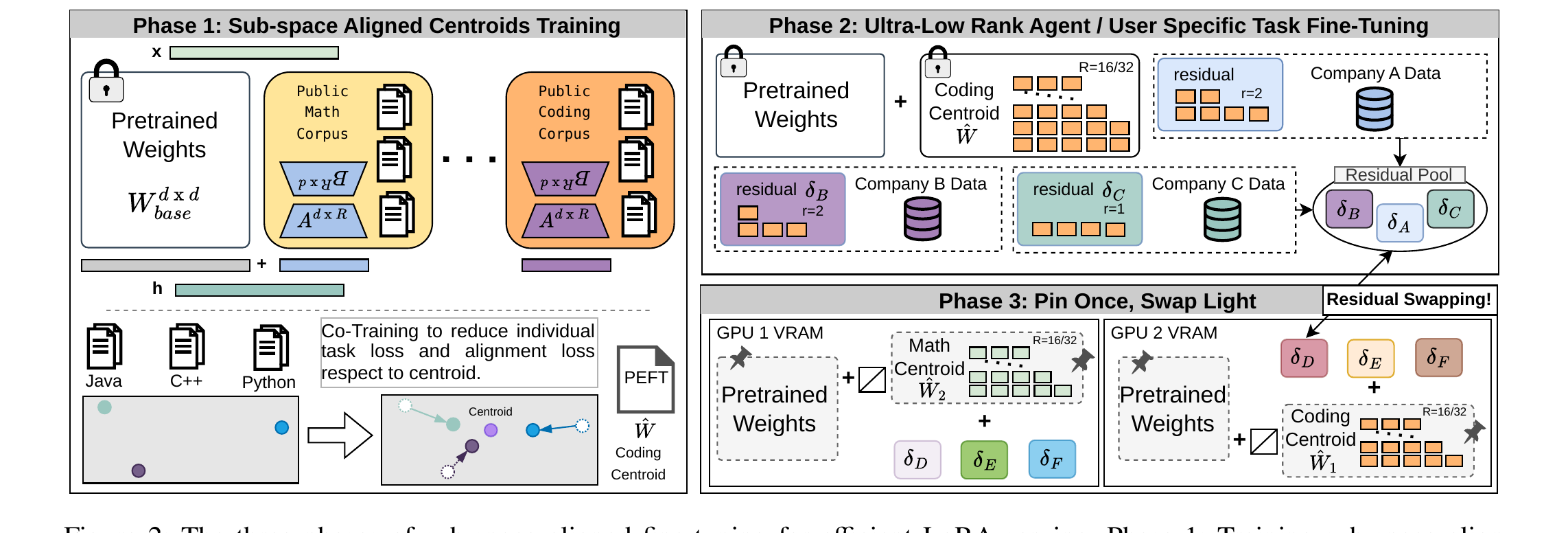

Figure 2 (paper Fig.2) makes the data-isolation boundary visually explicit: everything in the left “Phase 1” box touches only public corpora (Java/C++/Python code, public math problem sets); the moment private “Company A/B/C Data” appears (right side, Phase 2), it only ever gets composed with the already-frozen centroid, never fed back into training the centroid itself. This is the structural mechanism that lets SALT claim strict multi-tenant data isolation — a genuine advantage over prior shared-subspace methods that continually update the shared component using tenant data, silently entangling every existing tenant’s representation whenever a new one arrives.

The high-level intuition worth internalizing before the math: a rank-16 “domain centroid” pinned once in VRAM is shared infrastructure, amortized across every tenant in that domain — its one-time training cost and its VRAM footprint are paid once by the provider, not per-tenant. What actually needs to move over PCIe on a per-request basis is only the tiny residual, and because the residual is anchored to a semantically rich centroid rather than starting from nothing (or from a random projection), a rank as low as 1 turns out to be enough to recover most of what a fully independent rank-16 adapter would have achieved.

3. The centroid-residual decomposition, derived step by step

3.1 Why naive averaging of independent adapters doesn’t work

The most obvious way to get a “shared centroid” would be to train several independent LoRA adapters on related tasks and then simply average their weight updates: $\bar{W} = \frac{1}{M}\sum_i \Delta W_i$. The paper explains precisely why this fails, and Figure 5 (left panel) is the direct empirical evidence: independently trained adapters converge to distinct, unaligned local minima in weight-update space — even though GSM8K and SVAMP are both grade-school arithmetic word problems, their independently learned $\Delta W = BA$ matrices show near-zero cosine similarity, layer by layer, across the entire network depth. Averaging two near-orthogonal vectors doesn’t produce a meaningful shared direction; it produces something close to noise cancellation, destroying exactly the signal you wanted to keep.

Joint diagonalization (“Compress then Serve”) sidesteps this by extracting a shared basis mathematically from the already-trained independent adapters after the fact, rather than averaging them. But this creates the data-isolation and dynamic-scaling problems described in Section 1 — every tenant’s independently-trained (and therefore already privacy-sensitive) adapter has to be visible simultaneously to compute the joint decomposition, and a new tenant joining means recomputing the whole basis.

SALT’s answer is to skip both the after-the-fact averaging and the after-the-fact joint decomposition, and instead force alignment during training via an explicit optimization objective that trains the centroid and the task adapters jointly, so the centroid is never a passive average but an actively-optimized anchor that the task adapters are simultaneously being pulled toward.

3.2 Phase 1: the joint alignment objective, term by term

The core decomposition is deceptively simple to state:

$$\Delta W_i = \bar{W} + \delta_i \tag{eq. unlabeled, structural decomposition}$$

where $\bar{W}$ is the shared, domain-specific, task-agnostic centroid (high capacity, e.g. r=16, pinned permanently in VRAM) and $\delta_i = B_i'A_i'$ is the ultra-low-rank task residual (r≤2, the only thing that gets dynamically swapped per request). This decomposition alone is not the contribution — you could write this decomposition trivially for any two matrices that sum to $\Delta W_i$. The actual contribution is in how $\bar{W}$ is trained so that this decomposition is meaningful: so that $\delta_i$ really can be tiny without destroying accuracy.

Phase 1’s joint training objective, run entirely by the cloud provider on public, domain-specific data:

$$\min_{\{\Delta W_i\}, \bar{W}} \frac{1}{M}\sum_{i=1}^{M}\Big[ w_i\, \mathcal{L}_{task}(W_{base}+\Delta W_i; D_i) + \mathcal{L}_{task}(W_{base}+\bar{W}; D_i) + \lambda\, \mathcal{L}_{align}(W_{base}+\Delta W_i, \bar{W}) \Big] \tag{1}$$

Let’s unpack this term by term, because each piece is doing a distinct job:

• $w_i \, \mathcal{L}_{task}(W_{base}+\Delta W_i; D_i)$ — the standard task loss for the $i$-th individual public task adapter, evaluated on its own dataset $D_i$ (e.g., GSM8K for one adapter, SVAMP for another, both within the Math domain). This term alone is exactly what independent LoRA training would optimize. The weight $w_i \propto |D_i|$ reweights each task by its relative dataset size — without this, a task with a small dataset that gets cycled through more frequently during training could dominate the gradient signal disproportionately relative to its actual importance in the domain.

• $\mathcal{L}_{task}(W_{base}+\bar{W}; D_i)$ — this is the term that makes $\bar{W}$ an active participant rather than a passive average: the centroid itself, with no task-specific adapter added, is directly optimized to perform well on every task’s data $D_i$ in the domain. This is what makes the centroid genuinely a competent domain-level model on its own — recall Table 1’s “LoRA (Merged Dataset)” row, essentially a proxy for what a centroid-only model achieves, which is already competitive with (sometimes better than) independently-trained per-task LoRA on several datasets.

• $\lambda\, \mathcal{L}_{align}(W_{base}+\Delta W_i, \bar{W})$ — the alignment regularizer, which is the mechanism that actually solves the near-zero-cosine-similarity problem from Section 3.1 by explicitly penalizing divergence between each task adapter’s update and the centroid.

The alignment loss itself is an epsilon-stabilized matrix cosine similarity:

$$\mathcal{L}_{align}(\Delta W_i, \bar{W}) = 1 - \frac{\mathrm{Tr}(\Delta W_i^\top \bar{W})}{\|\Delta W_i\|_F \|\bar{W}\|_F + \epsilon} \tag{2}$$

Derivation and intuition. $\mathrm{Tr}(\Delta W_i^\top \bar{W})$ is the Frobenius inner product between the two weight-update matrices — treating each matrix as a flattened vector, this is exactly the ordinary dot product between them. Dividing by the product of Frobenius norms $\|\Delta W_i\|_F \|\bar{W}\|_F$ normalizes this to lie in $[-1, 1]$, exactly analogous to ordinary vector cosine similarity but applied to matrices via their Frobenius inner product structure. When the two matrices point in exactly the same direction (up to positive scaling), the ratio is 1 and $\mathcal{L}_{align} = 0$ — no penalty. When they’re orthogonal, the ratio is 0 and the loss is 1 — maximum penalty. When they point in opposite directions, the loss can reach 2. The $\epsilon = 10^{-8}$ term in the denominator exists purely for numerical stability: at initialization, $\bar{W} \approx 0$ (a freshly initialized LoRA-style centroid typically starts at or near zero, since $B$ is usually zero-initialized), which would make the raw ratio $0/0$ without the stabilizer.

Why cosine similarity specifically, rather than, say, an $L_2$ distance penalty $\|\Delta W_i - \bar{W}\|_F^2$? This is exactly the kind of design choice the paper leaves implicit but that’s worth working through explicitly, since it’s not discussed directly in the text. An $L_2$ penalty would force $\Delta W_i$ to be numerically close to $\bar{W}$ in magnitude as well as direction — but $\bar{W}$ is a high-capacity (r=16) matrix while $\Delta W_i$, being an individual public-data task adapter used only for the alignment signal (not the final residual), doesn’t need to match $\bar{W}$‘s scale, only its geometric direction, since what actually gets composed at serving time is a much smaller residual anchored to the centroid, not $\Delta W_i$ itself. Cosine similarity is scale-invariant by construction — it only cares about direction — which is precisely the property this training-time regularizer needs: pull every task’s independently-optimized direction toward the centroid’s direction, without also fighting the task loss over magnitude, since the task loss is already doing that job. The obvious risk of scale-invariance: two adapters could achieve perfect cosine alignment while having wildly different magnitudes, and the alignment loss alone provides no signal to prevent this — but since $\mathcal{L}_{task}$ is jointly minimized alongside $\mathcal{L}_{align}$ in the same objective, magnitude is still implicitly constrained by what actually helps the task loss.

3.3 Phase 2: why constraining to r≤2 is a feature, not just a compromise

Once $\bar{W}$ is fixed (frozen after Phase 1), Phase 2 adapts to a specific tenant’s private data by optimizing only the residual:

$$\min_{\delta_i} \mathcal{L}_{task}(W_{base} + \bar{W} + \delta_i; D^{(i)}_{private}) \tag{3}$$

Notice what’s frozen here: $W_{base}$ (the pretrained model) and $\bar{W}$ (the centroid) are both fixed constants in this optimization; only $\delta_i = B_i'A_i'$, with $r \le 2$, has any trainable parameters. This is the mechanism that structurally guarantees privacy isolation: private data literally cannot influence $\bar{W}$, because $\bar{W}$ isn’t in the optimization variables at all during Phase 2 — it’s baked in from Phase 1 and never touched again.

The paper makes an argument here that’s worth taking seriously rather than treating as a footnote: constraining the residual to r≤2 isn’t merely “the minimum capacity we can get away with” — it’s argued to be a structural regularizer in its own right. Because the residual genuinely lacks the parameter capacity to model the target task distribution independently (a rank-2 update to a $d\times d$ matrix, with $d$ typically in the thousands, is a tiny subspace), it is forced to lean on the pre-aligned centroid as a structural shortcut rather than trying to reinvent domain knowledge from scratch. This is a real, testable causal claim, and Table 6 (Section 5.4 below) is the paper’s evidence for it: a residual trained atop a subspace-aligned centroid vastly outperforms the identical low-rank residual trained atop a naively concatenated-data centroid, even though both centroids see the same total data — the only difference is whether the centroid’s direction was actively aligned with individual task adapters during training. If the residual’s tiny capacity alone were doing all the work regardless of centroid quality, this gap wouldn’t exist.

3.4 Phase 3: serving-time composition, and the inference-time scaling coefficient γ

At serving time, the final weight matrix used for tenant $i$‘s request is:

$$W_{final} = W_{base} + \gamma \bar{W} + \delta_i \tag{4}$$

The residual $\delta_i$ enters at full strength (coefficient 1, implicit), but the centroid gets scaled by $\gamma$. Why introduce a scaling knob for the centroid at all, when it was already directly optimized in Phase 1? The paper’s justification draws on the established idea of task arithmetic: composing multiple learned components (here, base weights + centroid + residual) can introduce interference at inference time that wasn’t visible when each component was trained/evaluated in isolation. $\gamma < 1$ dampens the centroid’s contribution (useful when interference is hurting a specific task), $\gamma > 1$ amplifies it. Table 4’s empirical sweep confirms this isn’t a purely theoretical concern: downstream accuracy follows a clear inverted-U shape across $\gamma \in [0.4, 1.2]$, peaking around $\gamma = 0.6$–$0.8$ and degrading noticeably at both extremes (GSM8K falls from a peak of 58.65% at $\gamma=0.8$ down to 48.83% at $\gamma=1.2$) — so the scaling coefficient is doing real corrective work, not just adding a redundant hyperparameter.

Why discretize $\gamma$ into a handful of predefined bins (e.g., $\{0.6, 0.8, 1.0\}$) rather than allowing a continuous per-request value? This is a serving-engine engineering decision with a clean rationale: continuously varying $\gamma$ per request would mean every single request potentially needs its own freshly-composed $(W_{base} + \gamma\bar{W})$ matrix, defeating the entire point of pinning a shared centroid — you’d be back to per-request weight composition overhead. By discretizing into bins, the serving frontend can group requests by their assigned $(\bar{W}, \gamma)$ pair and, for high-frequency bins, the provider can literally fuse the scaled centroid directly into the base weights once at node startup — after that, the node only ever swaps the tiny per-tenant residuals. Table 4’s finding that $\gamma \in \{0.6, 0.8, 1.0\}$ all cluster tightly in accuracy (average drop from peak of only 3.23% for math tasks, 1.53% for coding) is precisely what makes this discretization practical rather than a lossy approximation: the provider doesn’t need to search hard for the exact optimal $\gamma$, because the accuracy landscape is genuinely flat across a usable range. The one edge case the appendix’s fine-grained sweep (Figure 11 in the paper, not reproduced here) flags: AQuA (a multiple-choice math dataset, structurally different from the direct-generation math tasks) needs a higher $\gamma \approx 1.3$ to fully recover, foreshadowing the structural-bias limitation discussed in Section 7.

For rare, low-frequency requests where fusing isn’t worth the overhead, the paper notes the scaled centroid and residual can simply be concatenated offline into one standard adapter (e.g., an effective r=17 matrix) — letting the serving engine fall back to ordinary heterogeneous batching for the long tail, without needing a separate code path.

4. Automated centroid routing: algorithm and derivation

A practical multi-tenant system can’t assume every incoming tenant will tell you which domain centroid their data belongs to — and worse, if the data doesn’t cleanly belong to any existing centroid (genuinely out-of-distribution, OOD), forcing it onto the wrong centroid would actively hurt accuracy rather than help. SALT’s answer is a two-stage activation-profiling algorithm, run using only a small unlabeled sample of the tenant’s Phase-2 data.

4.1 Step-by-step algorithm walkthrough

Setup, done once offline at the end of Phase 1. For each centroid $\bar{W}_k$ in the library $\mathcal{C} = \{\bar{W}_1, \ldots, \bar{W}_K\}$, the provider passes that centroid’s own in-domain validation set through the model and records the empirical mean $\mu_{N,k}$ and standard deviation $\sigma_{N,k}$ of a displacement-norm statistic (defined next) — essentially calibrating “what does normal, in-domain activation behavior look like for this centroid.”

Step 1 — compute the displacement norm for the new data. Given a small unlabeled sample $D$ from the new tenant (the paper uses $|D_{profile}| = 100$ examples), and for each candidate centroid $k$, run the model with that centroid attached and compute:

$$N_k = \|h_k - h_{base}\|_2 \tag{5}$$

where $h_k$ is the final hidden state with centroid $\bar{W}_k$ applied, and $h_{base}$ is the hidden state with no adapter at all. This measures how much the centroid actually perturbs the model’s representation for this specific data — token-normalized to control for the fact that longer sequences accumulate more raw displacement regardless of domain relevance. Intuitively: if the tenant’s data is genuinely math-flavored, attaching the Math centroid should meaningfully shift the hidden state relative to the unmodified base model, because the centroid’s learned direction is actually relevant and gets activated; unrelated data shouldn’t move the representation much in any centroid’s particular direction.

Step 2 — OOD rejection via deviation. Compute the standardized deviation from each centroid’s calibrated baseline:

$$Z_{N,k} = \frac{|N_k - \mu_{N,k}|}{\sigma_{N,k}} \tag{6}$$

This is a standard z-score: how many standard deviations away from “typical in-domain displacement for centroid $k$” is the new data’s observed displacement. If the minimum deviation across every centroid in the library still exceeds a strict threshold ($\min_k Z_{N,k} > \tau_N$, e.g. $\tau_N = 2.0$, corresponding to roughly a 95% confidence interval), the data is flagged as lacking geometric overlap with any available centroid — it’s OOD, and the system falls back to training a standard, non-anchored LoRA adapter for this tenant rather than forcing a poor-fit centroid onto it.

Step 3 — expert routing among in-domain candidates. If the OOD check passes (some centroid is plausibly relevant), a second, more discriminating comparison is needed, because raw displacement norms $N_k$ can fluctuate simply due to prompt structure or vocabulary complexity, independent of true domain alignment. The paper computes a dominance ratio:

$$R_k = \frac{N_k}{\frac{1}{K-1}\sum_{j\ne k} N_j}, \qquad k^* = \arg\min_k \frac{|R_k - \mu_{R,k}|}{\sigma_{R,k}} \tag{7}$$

Why a ratio against the average of all other centroids, rather than just picking $\arg\max_k N_k$ directly?** This is exactly the kind of design choice worth interrogating. If a tenant’s data happens to produce uniformly large displacement across every centroid (perhaps because it’s simply longer or more complex text, unrelated to genuine domain fit), a raw $\arg\max$ would still pick some centroid confidently, even though none of them is genuinely a better relative fit than the others. The ratio $R_k$ normalizes each centroid’s displacement against the average displacement induced by all the others, which cancels out exactly this kind of length/complexity-driven inflation that would otherwise affect every centroid roughly equally — what’s left after normalizing is closer to a measure of relative domain fit, which is what routing actually needs.

4.2 The full algorithm as pseudocode

Algorithm 1: Automated Centroid Routing
Input: unlabeled tenant sample D, centroid library C = {W̄_1, ..., W̄_K},
       pre-calibrated (μ_N,k, σ_N,k, μ_R,k, σ_R,k) for each k,
       thresholds τ_N, τ_R (e.g., both 2.0)
Output: selected centroid index k*, or FALLBACK (standard LoRA)

 1: for k = 1 to K do
 2:     run model with W̄_k attached on sample D
 3:     h_k ← final hidden state (token-normalized)
 4:     h_base ← final hidden state with no adapter attached
 5:     N_k ← ‖h_k − h_base‖_2                     // Eq. 5
 6: end for
 7: Z_N_min ← min_k |N_k − μ_N,k| / σ_N,k           // Eq. 6, best-fit OOD deviation
 8: if Z_N_min > τ_N then
 9:     return FALLBACK                              // OOD: no centroid fits well enough
10: end if
11: for k = 1 to K do
12:     R_k ← N_k / ( (1/(K−1)) · Σ_{j≠k} N_j )      // Eq. 7, dominance ratio
13:     Z_R,k ← |R_k − μ_R,k| / σ_R,k
14: end for
15: k* ← argmin_k Z_R,k
16: if Z_R,k* > τ_R then
17:     return FALLBACK                              // ambiguous / blended domain
18: end if
19: return k*                                        // route to W̄_k* for Phase 2

Table 3’s validation of this algorithm on six held-out datasets is a clean illustration of exactly the intended behavior: AQuA and MultiArith (both math, both held out from Phase 1 training so this genuinely tests generalization, not memorization) correctly route to the Math centroid with low $Z_R$ (0.94 and 0.11); CodeSearchNet and APPs correctly route to Code ($Z_R$ = 0.49 and 0.39); and — the important negative-control case — two XNLI language-classification splits (German, Spanish), which have no real relationship to either math or code, both correctly trigger the OOD fallback, with $Z_N$ = 2.28 and 2.32, both comfortably above the $\tau_N = 2.0$ threshold. Correctly rejecting genuinely unrelated data, not just correctly accepting related data, is the harder and more informative half of this validation.

5. Design choices worth interrogating: why, what’s the alternative, where does it fail

Why train the alignment penalty jointly with the task loss in one combined objective (Eq. 1), rather than a two-stage pipeline — first train independent adapters normally, then post-hoc project them onto a shared basis? The obvious alternative (train adapters to convergence independently, then align afterward, closer in spirit to “Compress then Serve”) would let each stage be optimized more simply in isolation. The paper’s design implicitly rejects this because a post-hoc projection can only find the best shared subspace given whatever geometry the independently-trained adapters already happened to converge to — and Section 3.1’s near-zero cosine similarity finding shows that geometry is essentially arbitrary/unaligned to begin with, so a post-hoc projection is trying to find structure in what is, from the perspective of downstream residual composition, close to noise. Joint training instead actively shapes where the adapters converge during optimization, using the alignment gradient to steer them toward a common direction from the start, rather than accepting whatever direction gradient descent happens to find and trying to fix it afterward. Where this joint approach could fail: it couples the centroid’s optimization trajectory to every individual task adapter’s trajectory simultaneously (Table 13’s training-cost analysis shows this scales as $O(M)$ in both memory and per-step latency with the number of adapters $M$ trained jointly), so onboarding a genuinely new domain still requires a full joint retraining pass with all of that domain’s public tasks — it’s cheaper than per-tenant retraining, but it’s not free, and it’s a real practical constraint on how many domains a provider can realistically maintain and refresh.

Why fix the residual rank ceiling at r≤2 rather than exposing rank as a tunable per-tenant knob? A tunable per-tenant rank would let a provider offer higher fidelity to tenants willing to pay for more swap bandwidth — genuinely more flexible on paper. The paper’s implicit answer is visible in the serving-efficiency argument itself: the entire throughput win (Section 6.4 below) comes from uniformly tiny swap payloads enabling larger continuous batches and less PCIe contention across all concurrent tenants simultaneously; if some tenants used r=8 or r=16 residuals while others used r=1, the serving engine would be back to handling a heterogeneous, unpredictable swap-size distribution, undermining exactly the scheduling predictability that the memory-footprint reduction is trying to buy. The r≤2 ceiling is as much a serving-engine design constraint as an accuracy-vs-cost trade-off. Where it fails: Section 6 (Limitations) documents that tasks needing a genuinely different output format than what the domain generally requires — e.g., multiple-choice evaluation (AQuA) sitting inside an otherwise direct-generation-dominated Math domain — can be actively hurt, because the r≤2 residual, forced to lean on a centroid optimized mostly for direct generation, simply lacks the capacity to override that structural bias when the task genuinely needs to diverge from it.

Why use a hierarchical library of multiple domain-specific centroids (Math, Code, …) rather than one single universal centroid covering everything? Appendix A.3’s multi-domain interference experiment (Table 12, not reproduced as a figure here but worth stating directly) answers this empirically: expanding a single centroid’s training data from 2 tasks to 6 tasks (mixing Math with unrelated Code and Language tasks) monotonically degrades downstream accuracy on the original in-domain tasks — GSM8K drops from 46.65% to 43.92%, SVAMP from 74.17% to 70.0%, as more heterogeneous data is folded in. This directly rules out the tempting simplification of a single all-purpose centroid: cramming semantically unrelated domains into one shared basis causes negative transfer, the same failure mode a naive single global model faces, just relocated into the centroid rather than the base model. The paper’s approach requires the provider to partition tasks into “sufficiently coherent domains” in advance, which is itself a real design burden the paper doesn’t offer an automated solution for — domain partitioning is left as a manual/heuristic step, not something SALT’s algorithm decides for you.

Why is the residual optimized against the unscaled centroid in Phase 2 (Eq. 3 has no $\gamma$), while $\gamma$ is only introduced at serving time (Eq. 4)? This is a subtle sequencing choice with a real consequence. If $\gamma$ were baked into Phase 2 training, the residual would learn to compensate for one specific scaling of the centroid, and any post-hoc adjustment of $\gamma$ at serving time (e.g., a provider deciding a different bin better balances multi-task interference across the current mix of concurrently-served tenants) would silently break that tenant’s residual, since it was never trained to work with any $\gamma \ne 1$. By training the residual against the unscaled centroid and only introducing $\gamma$ as a serving-time composition parameter, the provider retains the freedom to retune $\gamma$ system-wide, per domain, without invalidating any already-trained tenant residual. The cost: Table 4 shows this decoupling isn’t entirely free — performance does depend measurably on $\gamma$, so the provider still has to choose reasonably (empirically, $\gamma \in [0.6, 0.9]$), it’s just that the residual doesn’t need retraining when that choice changes.

6. Results, reproduced with commentary

6.1 Main comparison: task accuracy and memory footprint on Mistral-7B-v0.3

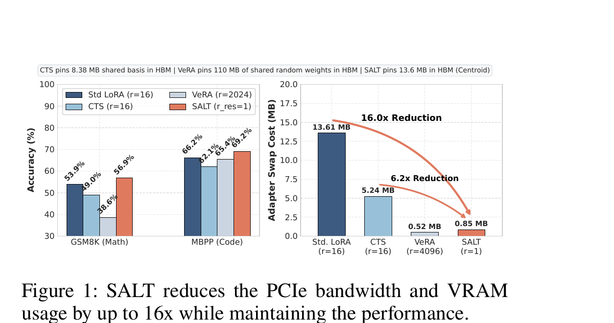
Figure 1 (paper Fig.1) is the paper’s headline claim compressed into two panels. Left panel: on GSM8K, SALT’s r_res=1 residual (56.9%) beats every baseline including full rank-16 Standard LoRA (53.9%) — a genuinely counter-intuitive result worth sitting with, since SALT is using less trainable capacity per tenant than the method it’s beating. On MBPP, the ordering is SALT (69.2%) > Standard LoRA (66.2%) > VeRA (65.4%) > CTS (62.1%) — SALT wins, but the margin over the strongest baseline is narrower here than on GSM8K. Right panel translates this into the metric that actually governs serving cost: adapter swap cost in MB. Standard LoRA at r=16 costs 13.61 MB per swap; SALT’s r=1 residual costs 0.85 MB — a 16.0x reduction — while CTS (5.24 MB, 6.2x smaller than Standard LoRA but still 6x larger than SALT) and VeRA (0.52 MB, even smaller than SALT, but recall VeRA needs its enormous 110 MB basis permanently pinned to reach this) round out the comparison. The full picture only makes sense when you read the two panels together: SALT is simultaneously matching-or-beating accuracy and achieving close to the smallest per-request swap cost among all real (non-degenerate) competitors.

The full numeric breakdown, Table 1 in the paper, is worth walking through directly because the aggregate story hides some real texture:

Method	Rank	Pin (MB)	Swap (MB)	GSM8K‡	SVAMP‡	MBPP‡	SPIDER‡
Standard LoRA	r=16	0.00	13.61	53.88	66.25	26.75	21.34
VeRA	r=4096	109.05	1.05	40.79	60.83	26.50	31.53
CTS (JD-Full)	r=16	8.38	5.24	49.02	62.08	9.25	3.47
SALT (r=1)	r=1	13.63	0.85	56.88 (+7.2)	69.17 (+5.8)	27.25 (+11.5)	56.59 (+26.3)

(‡ = datasets used for both Phase 1 centroid training and Phase 2 residual tuning — the “seen in-domain” setting; the paper also reports “unseen in-domain” and “zero-shot transfer” settings, discussed below.)

The SPIDER column is the most dramatic single number in the entire table: CTS collapses to 3.47% at r=16 (essentially non-functional for text-to-SQL) while SALT reaches 56.59% at r=1 — a 53-point gap. This isn’t a fluke of one baseline being poorly tuned; Appendix A.5 (Table 14, Section 5.4 below) shows this same pattern holds specifically because SPIDER is unusually sensitive to whether the centroid is subspace-aligned or naively concatenated, and the paper documents a specific, concrete failure mode (Listing 1) explaining exactly why.

Generalization beyond seen tasks. The paper deliberately structures its evaluation into three settings of increasing difficulty: Seen In-Domain (residual tuned on the same datasets the centroid was trained on), Unseen In-Domain (residual tuned on held-out datasets from the same domain — MultiArith, AQuA, APPs), and Zero-Shot Transfer (a residual trained on MBPP evaluated directly on HumanEval with zero additional training). The MultiArith numbers are the most striking evidence for genuine generalization, not overfitting to the exact training distribution: SALT reaches 86.21% versus Standard LoRA’s 30.35% at r=16 — a +55.86 percentage point gap on a dataset never seen during either phase of SALT’s training. This is strong evidence that what the centroid is actually capturing is transferable domain structure (grade-school arithmetic reasoning patterns generally), not memorized answers to the specific GSM8K/SVAMP training sets.

6.2 Cross-architecture consistency

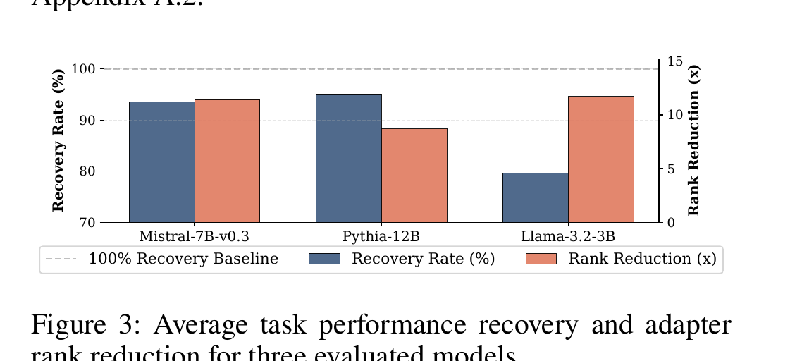
Figure 3 (paper Fig.3) checks whether the Mistral-7B results generalize across model families and scales — Mistral-7B-v0.3, Pythia-12B, and Llama-3.2-3B, three genuinely different architectures (different attention configurations, different pretraining corpora, an order-of-magnitude parameter range). The recovery rate (SALT’s accuracy as a fraction of what full rank-16 Standard LoRA achieves) stays in the 80–95% range across all three, while rank reduction ranges from 9x to 11.5x. The one place worth flagging honestly: Llama-3.2-3B shows the lowest recovery rate (~80%) paired with the highest rank reduction (~11.5x) among the three — a real trade-off point, not a uniformly dominant result, suggesting that at the smallest tested model scale, squeezing to the most extreme compression does cost a bit more accuracy than at larger scales. This is consistent with a broader, intuitive pattern in LLM compression research: smaller models generally have less redundant capacity to sacrifice before compression costs start to bite.

6.3 Serving efficiency: swap footprint, latency, and end-to-end vLLM throughput

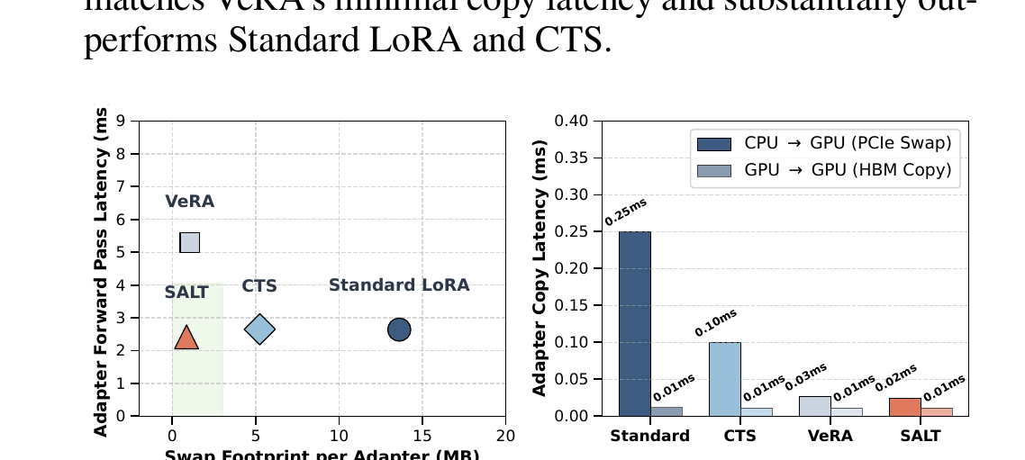
Figure 4 (paper Fig.4), left panel, is a genuinely useful two-axis view most papers in this space don’t provide together: swap footprint on the x-axis, forward-pass latency on the y-axis. SALT sits in the bottom-left — smallest footprint and lowest forward-pass latency simultaneously, whereas VeRA, despite a comparably tiny reported swap footprint, pays a much higher forward-pass latency (its large frozen random basis still has to be multiplied through at inference time even though it isn’t swapped). Right panel breaks down the two latency components that matter for swap-heavy serving: CPU→GPU PCIe swap (the genuinely expensive one, 0.25ms for Standard LoRA at r=16) versus GPU→GPU HBM copy (cheap regardless of method, all under 0.02ms). SALT’s PCIe swap latency (0.02ms) is essentially at the VeRA/CTS floor and an order of magnitude below Standard LoRA’s 0.25ms — this is the direct, measured consequence of the 16x memory reduction translating into real wall-clock savings on the actual expensive resource, not just a theoretical byte-count improvement.

The end-to-end vLLM integration numbers (Table 2 in the paper) confirm these micro-benchmark gains survive contact with a real serving stack: at N=512 concurrent adapters under PCIe bandwidth pressure, vLLM+SALT reaches 54.46 req/s versus vanilla vLLM’s 43.42 req/s (+25.4%); under VRAM capacity pressure at the same concurrency, 38.41 vs 32.59 req/s (+17.9%). Notably, these gains come without any custom kernel — SALT relies purely on standard additive matrix operations ($W_{base} + \gamma\bar{W} + \delta_i$ is just ordinary matrix addition), which is precisely why it plugs directly into vLLM’s existing SGMV-based adapter-serving pipeline, whereas the paper explicitly notes VeRA and CTS’s specialized matrix structures require non-standard serving pipelines and had to be excluded from this particular end-to-end comparison for that reason — a genuine practical advantage for real-world deployability that a pure accuracy-vs-memory comparison would miss entirely.

6.4 Does the alignment penalty actually align adapters, geometrically?

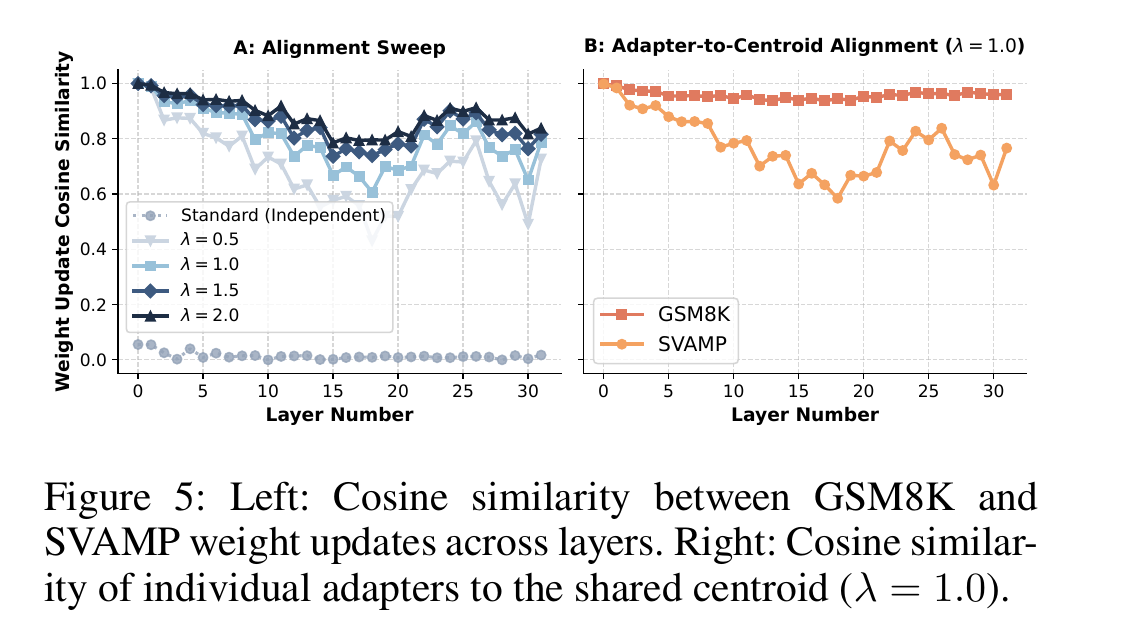
Figure 5 (paper Fig.5) is the direct mechanistic validation behind the entire method — it’s answering “does the alignment loss (Eq. 2) actually do what it’s supposed to do, geometrically, or is the accuracy improvement coming from somewhere else?” Left panel: the “Standard (Independent)” curve (adapters trained with no alignment penalty at all, $\lambda=0$ effectively) sits essentially at zero cosine similarity across every layer — this is the direct visual confirmation of the Section 3.1 claim. As $\lambda$ increases from 0.5 to 2.0, the curves climb monotonically and substantially, reaching 0.7–0.9+ similarity across most layers at $\lambda=2.0$. Right panel shows the same effect from the other side: individual adapters’ similarity to the centroid itself (not to each other) climbs to consistently above 0.9 for GSM8K and shows a somewhat noisier but still clearly elevated pattern for SVAMP, confirming both the task adapters and the centroid genuinely converge into a shared geometric neighborhood, not just that the two task adapters happen to align with each other while drifting away from the centroid.

6.5 The alignment-penalty sensitivity sweep, and why moderate λ is enough

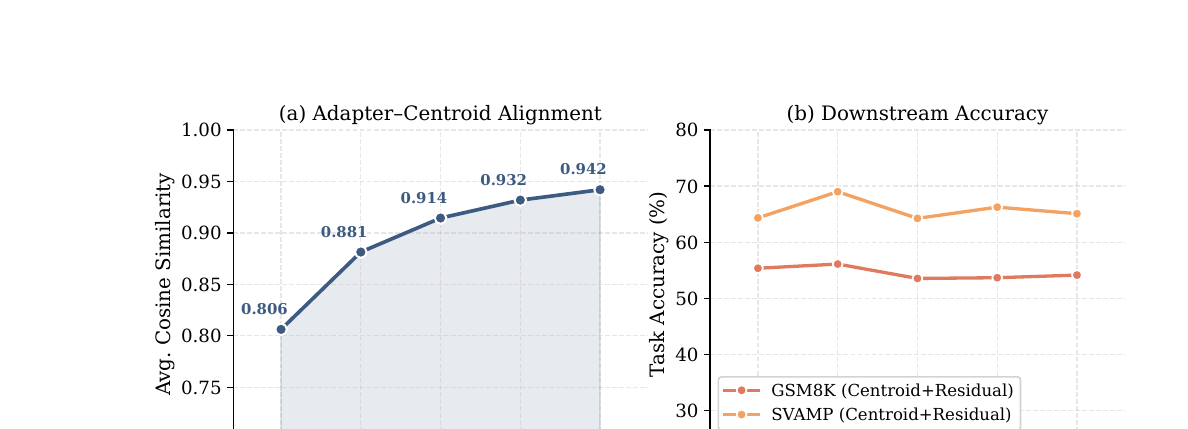
Figure 6 (paper Fig.6) sweeps $\lambda$ from 0.5 to 2.5 and plots both the geometric effect (panel a: cosine similarity climbs from 0.806 to 0.942, essentially saturating) and the downstream effect (panel b: task accuracy for GSM8K and SVAMP under Centroid+Residual composition). The genuinely informative finding here is what doesn’t happen: despite the alignment penalty growing substantially stronger (nearly tripling from 0.5 to 2.5), downstream accuracy stays essentially flat across the whole sweep. This is a real, somewhat reassuring negative result: it means the alignment constraint isn’t fighting the task objective in a way that trades off task quality for geometric tidiness — you can push alignment fairly hard without paying an accuracy cost, at least within the domain and task set tested here. It also means the specific value of $\lambda$ isn’t a fragile hyperparameter a provider needs to tune carefully per domain; a moderate value in the middle of the tested range is a safe default.

7. Limitations, stated and unstated

The paper is direct about several limitations, and Section 6 of the paper is worth quoting in spirit rather than glossing over. First, the structural bias against orthogonal task formats: because Phase 1 alignment enforces a strict geometric intersection across tasks within a domain, a task whose natural output format genuinely diverges from what dominates the domain — the paper’s own example is multiple-choice evaluation (AQuA) sitting inside a Math domain otherwise dominated by direct-generation tasks — can suffer, because the r≤2 residual’s tiny capacity isn’t enough to override the centroid’s learned bias toward the dominant format. Table 1 shows this concretely: AQuA is the one dataset in the entire Mistral-7B comparison where SALT trails Standard LoRA at matched or lower rank (31.37% vs 34.80% at r=2, a -5.3 point gap).

Second, the evaluation is restricted to exactly two domains (math and coding). This is a real scope limitation worth being honest about: the paper’s own multi-domain interference experiment (Appendix A.3, Table 12, discussed in Section 5 above) shows negative transfer when domains are mixed carelessly, which means the paper’s core positive results are demonstrated only within domains the authors already knew were internally coherent — it doesn’t tell you how to discover coherent domain boundaries for a genuinely novel deployment with dozens of heterogeneous tenant verticals, which is exactly the situation a real LLMaaS provider would face.

Third, and explicitly flagged as open future work by the authors themselves: extending SALT to Mixture-of-Experts architectures remains unsolved. The paper’s own reasoning is sound and worth restating: MoE’s sparse, disjoint expert-routing paths make establishing one unified geometric subspace across experts “mathematically complex without additional memory cost” — a single shared centroid concept doesn’t obviously transfer to a setting where different tokens route through entirely different expert subnetworks, and the paper offers no partial solution or even a sketch of one.

What the paper doesn’t discuss, and is worth flagging independently: the offline calibration cost of centroid routing (Section 4) requires the provider to have already collected in-domain validation statistics ($\mu_{N,k}, \sigma_{N,k}, \mu_{R,k}, \sigma_{R,k}$) for every centroid before routing can work at all — this is a one-time cost per centroid, but it means adding a new centroid to the library isn’t just “train it” (Phase 1), it also requires running this calibration pass, and the paper never discusses how much data or compute that calibration itself requires, nor how sensitive routing accuracy is to how well-calibrated those baseline statistics are.

8. Critical analysis

Weaknesses and flaws specific to this paper. First, the routing algorithm’s OOD/expert-routing thresholds ($\tau_N = 2.0$, $\tau_R = 2.0$) are presented as fixed, universal defaults tied to “95% confidence interval” framing, but this framing implicitly assumes the underlying displacement-norm and dominance-ratio statistics are approximately Gaussian around their calibrated means — an assumption the paper never actually tests. If the true distribution of $N_k$ or $R_k$ for a given centroid is meaningfully skewed or heavy-tailed (plausible, since these are derived from complex nonlinear model activations, not raw data), a “2 standard deviations” cutoff doesn’t actually correspond to a genuine 95% confidence interval, and the routing algorithm’s false-accept/false-reject rates could be systematically miscalibrated in ways the paper’s six-dataset validation (Table 3) is too small a sample to detect. Second, the accuracy comparison against VeRA in Table 1 uses VeRA at ranks up to r=4096 to be “competitive” — but the paper’s own framing (VeRA needs a large basis “since only diagonal scaling vectors are learned”) means the comparison at, say, r=1024 (VeRA’s smallest tested configuration, which still costs 27.26 MB pinned) versus SALT’s 13.63 MB pinned centroid isn’t actually an apples-to-apples memory comparison at the low end — VeRA’s smallest viable configuration already pins roughly 2x SALT’s centroid, and the paper doesn’t test whether an even smaller VeRA configuration (r < 1024) could be viable with different tuning, leaving open whether the reported VeRA numbers represent VeRA’s true minimum-memory operating point or simply the smallest configuration the authors happened to test.

Limitations the authors understate or omit. The paper repeatedly frames the r≤2 residual constraint as purely a capacity-vs-cost design choice, but understates how much this constraint interacts with domain granularity choices the provider has to make manually — the AQuA failure case (Table 1) is presented as an isolated example, but the underlying mechanism (residual capacity insufficient to override centroid bias for structurally divergent tasks) is generic, and the paper doesn’t characterize how common or predictable this failure mode is across a broader task distribution than the eight datasets tested — a provider deploying this in production has no principled way, from what’s in the paper, to predict in advance which new tenant tasks will hit this failure mode before actually trying them. Second, the paper’s training-cost scaling analysis (Appendix A.4, Table 13) shows Phase 1 cost grows as $O(M)$ in the number of jointly-trained task adapters, and reports this scales “comfortably” up to M=50 adapters on a single H100 — but a real domain (e.g., “Coding” broadly) plausibly needs to absorb far more than 50 distinct public task datasets to be genuinely representative of the diversity of coding tasks a production platform would serve, and the paper doesn’t extrapolate or discuss what happens to Phase 1 training cost or centroid quality as $M$ grows into the hundreds, which is the more realistic regime for a mature domain.

Concrete, specific improvement suggestions. (1) Directly test the Gaussian-approximation assumption underlying the routing thresholds — report the actual empirical distribution shape of $N_k$ and $R_k$ across a larger and more diverse set of held-out datasets than the six tested in Table 3, and if the distributions are meaningfully non-Gaussian, replace the fixed z-score thresholds with a non-parametric alternative (e.g., empirical percentile cutoffs) that doesn’t rely on the normality assumption. (2) Run an ablation specifically isolating whether the AQuA-style structural-format failure mode can be mitigated by a slightly higher residual rank (e.g., r=3 or r=4, still far below r=16) specifically for tasks flagged during Phase 2 as poorly served by r≤2 — this would clarify whether the failure is fundamentally about the r≤2 ceiling or about the alignment penalty’s strength, since these are currently confounded in the paper’s design. (3) Report Phase 1 training-cost scaling and downstream centroid quality at $M$ in the hundreds, not just up to 50, since this is the realistic scale for mature production domains, and the current $O(M)$ scaling claim’s “comfortable” framing is only validated at a scale roughly an order of magnitude below what a mature deployment plausibly needs. (4) Extend the multi-domain interference study (currently only 2/4/6-task mixtures within a hand-picked set) to test whether a hierarchical centroid structure (e.g., a broad “STEM” centroid with Math and Code as sub-centroids beneath it) could recover some of the negative-transfer cost of over-broad domains while still amortizing more shared structure than fully separate domains — this would directly address the domain-partitioning burden flagged in Section 7 as unsolved.

9. Reproducibility notes

The paper documents its experimental setup with reasonable, if not maximal, granularity: exact optimizer settings (AdamW, weight decay 0.01, cosine decay schedule, 3% linear warmup, gradient clipping at norm 1.0), exact dataset splits and sizes (Appendix A.1, Table 7, down to the exact train/valid/test counts for every one of the eight datasets used), and exact prompt templates for the coding tasks (Figures 7 and 8 in the paper, reproduced verbatim). The three base model families (Llama-3.2-3B, Mistral-7B-v0.3, Pythia-12B) are all publicly available checkpoints, and all evaluation datasets (GSM8K, SVAMP, MultiArith, AQuA, MBPP, SPIDER, APPs, HumanEval, plus XNLI for the OOD routing test) are standard, publicly released benchmarks with well-documented evaluation protocols, which meaningfully reduces the risk of an unfair or hard-to-replicate baseline comparison. The one open reproducibility gap as of this review: the paper does not state whether code will be released, and no code repository is linked in the preprint — so while the algorithmic description (Eqs. 1–7, Algorithm 1 as reconstructed above) is precise enough to reimplement the core method, the exact hyperparameter choices for baselines (VeRA’s specific rank sweep methodology, CTS’s joint-diagonalization implementation details) would need to be independently re-derived from the cited prior work rather than directly reused from this paper’s own code.

10. Where this sits in the broader low-rank adaptation landscape

If you’ve been following this blog’s coverage of low-rank and PEFT methods, SALT is worth placing directly against several threads already covered here. LoRA itself (the foundational low-rank decomposition this entire line of work builds on) treats rank purely as a capacity dial with no serving-efficiency mechanism built in. PiSSA and related SVD-initialization methods extract structure directly from the base model’s own weights via SVD at initialization time — a fundamentally different source of structure (intrinsic to the pretrained weights) than SALT’s centroid, which is learned from task data. VeRA, discussed extensively throughout this review as SALT’s direct point of comparison, represents the opposite extreme on the isolation-vs-expressivity spectrum: perfect tenant isolation via a frozen random basis, at the cost of needing enormous basis dimensionality to be competitive. HydraLoRA (a single shared $A$ matrix with multiple task-specific $B$ matrices via mixture-of-experts routing) and LoraHub (dynamic composition of independent adapters at inference time) both pursue a shared-component idea, but neither incorporates an explicit training-time geometric alignment objective the way SALT’s Eq. 2 does — they share structure by architectural constraint (a shared matrix, or post-hoc composition) rather than by actively training independently-initialized components toward a common direction. What makes SALT distinctive relative to all of these is the specific combination of (a) an explicit, differentiable alignment loss during joint training rather than an architectural sharing constraint or a post-hoc basis extraction, and (b) a serving-efficiency argument built directly into the method’s design from the start (uniform tiny residual size, γ-bin discretization for fusion, standard-kernel compatibility with vLLM) rather than treated as an afterthought bolted onto an accuracy-first method. For a practitioner building a genuinely multi-tenant LoRA-serving platform today, this paper’s own numbers suggest SALT is the strongest available option specifically when tenants can be grouped into a moderate number of internally coherent domains and per-tenant fine-tuning data is private — precisely the situation most LLMaaS platforms with customer-specific fine-tuning already operate in.

11. Conclusion

SALT’s central bet is that the usual trade-off framing — “higher rank for better accuracy” versus “lower rank for cheaper serving” — is itself the wrong axis to optimize, because it conflates two genuinely separable things: how much domain knowledge an adapter needs to encode, and how much tenant-specific deviation from that domain it needs to capture. By training a high-capacity, actively geometry-aligned centroid once per domain (paid for once, amortized across every tenant, and never touched by private data) and letting each tenant’s residual be as small as r=1 (because it only has to capture the tenant-specific delta, not the whole domain), SALT recovers most or all of what a full rank-16 independent adapter would have achieved, while cutting the actual per-request swap cost that governs multi-tenant serving throughput by up to 16x. The mechanics that make this work are genuinely well-motivated end to end: an epsilon-stabilized cosine alignment loss that solves a real, measured geometric-divergence problem (Figure 5’s near-zero baseline similarity), a two-stage z-score-based routing algorithm that correctly separates in-domain from out-of-distribution tenant data without requiring labels, and a discretized γ-scaling mechanism that keeps serving-time composition compatible with standard batched-kernel serving engines rather than requiring custom infrastructure. The honest caveats — a structural bias against tasks whose format diverges from a domain’s dominant pattern, an evaluation scope limited to two hand-picked coherent domains, unresolved extension to Mixture-of-Experts architectures, and untested assumptions underlying the routing algorithm’s confidence thresholds — don’t undercut the core contribution, but they’re exactly the right places to look before assuming the reported 16x memory reduction and 51% throughput gain transfer unchanged to a deployment with dozens of heterogeneous verticals rather than the two clean domains tested here.