Fine-Grained Compute-Communication Overlap for MoE: Hiding All-to-All Behind GEMM with Tile-Level Signaling

Review date: 2026-08-06 Author: Zhongzhu Zhou Paper reviewed: Fine-grained Computation-Communication Overlap via Tile-level Signaling and Scheduling for Mixture-of-Experts Paper authors: Minyu Cui, Anna Wingkvist, Morgan Ericsson (Linnaeus University) arXiv: 2607.19539 Venue/Status: To appear at ICPP 2026 (55th International Conference on Parallel Processing)

1. Why this paper, and what problem is it actually solving

Start with a fact that anyone who has profiled a Mixture-of-Experts (MoE) forward pass on multiple GPUs already knows in their bones: roughly half of the wall-clock time in a distributed MoE layer can be spent not computing anything, but waiting for tokens to move between GPUs. Sparse MoE architectures were supposed to solve a scaling problem — grow model capacity (more experts, more parameters) without proportionally growing the compute each token actually touches. And at the level of FLOPs, they deliver: a token routed to top-k out of E experts only pays for k/E of a dense layer’s compute. But in a distributed deployment, “only compute a little” quietly trades one bottleneck for another. To route a token to its assigned expert, you first have to ship it there — and to get the output back, you have to ship it back. Those two shipping operations are collective communication calls (all-to-all), and on modern hardware, all-to-all is expensive precisely because GPU compute throughput has raced ahead of interconnect bandwidth. A100-class GPUs deliver hundreds of TFLOPs of tensor-core throughput, but NVLink between a GPU pair on the platform used in this paper caps out around 100 GB/s one-way. Compute grew geometrically; the wires didn’t keep up.

The textbook fix for “communication is slow, compute is available” is to overlap the two — run communication concurrently with independent computation so the slower of the two, not their sum, determines wall-clock time. This is not a new idea in this paper; overlapping decomposition-based (chunk the GEMM and the collective, pipeline the chunks) and fusion-based (weld computation and communication into one kernel) techniques have existed for years, and the paper is careful to survey both families in its related work. What makes this paper worth a full read rather than a skim, though, is a specific technical claim buried in its introduction: existing overlap methods either (a) decompose along a single tensor dimension because NCCL’s collective APIs require contiguous buffers, which forces communication granularity to be misaligned with the GEMM’s natural tile structure — so tile-level overlap is “hard to achieve through decomposition alone” — or (b) achieve fine granularity by fusing computation and communication into a single monolithic kernel, at the cost of “intrusive engineering, including custom barriers, inter-rank atomic protocols, and per-target kernel specialization.” Neither camp gets you tile-granularity overlap without either misalignment or invasive kernel surgery.

This paper’s answer is a third path: keep the GEMM and the communication as two entirely separate, ordinary-looking kernels — no fusion, no custom barrier protocol threaded through the GEMM’s main loop — but coordinate them through lightweight, per-tile, device-resident “ready” flags, and run them concurrently on disjoint sets of streaming multiprocessors (SMs) so neither steals cycles from the other. The one piece of real engineering effort goes into a data-layout trick — reordering the GEMM’s input rows so that every output tile has a single, statically-known destination rank — which is what makes tile-granular, per-tile-triggered transfer possible in the first place without per-row routing logic on the hot path. The result, measured on a 4-GPU A100 node against four state-of-the-art MoE systems (FasterMoE, Tutel, Megatron with CUTLASS GroupGEMM, Megatron with Transformer Engine), is up to 2.64x end-to-end and 2.74x MoE-layer speedup, with per-token outputs matching the sequential baseline to within FP16 rounding noise. If you work on distributed LLM training or inference systems, MoE routing, or GPU kernel-level overlap engineering, this is a clean, mechanistically legible design worth understanding in full — not because the idea of “overlap compute and communication” is new, but because the specific data layout and scheduling discipline that makes tile-granular overlap practical without kernel fusion is the interesting engineering content here.

2. Prerequisites: what you need to know before the method makes sense

2.1 Mixture-of-Experts, briefly

In a standard (dense) transformer block, every token passes through the same feed-forward network (FFN), so total FFN compute scales linearly with model size — bigger model, proportionally more FLOPs per token. A Mixture-of-Experts layer breaks that coupling. Instead of one FFN, an MoE layer has E “expert” sub-networks (each usually itself an FFN) and a small gating/router network. For each token, the router computes a probability distribution over the E experts and picks the top-k (commonly k=2), and the layer’s output is the gate-weighted sum of just those k experts’ outputs. Since only k out of E experts ever touch a given token, the active compute per token stays roughly constant even as E (and therefore total parameter count) grows — this is precisely how MoE architectures like Switch Transformer, GShard, and modern trillion-parameter LLMs scale capacity without scaling per-token FLOPs proportionally.

2.2 Distributed MoE execution: five steps, two of them communication

When E experts don’t fit on one GPU (or you simply want expert-parallelism for other reasons), you place different experts on different ranks (this paper uses “rank” and “GPU” interchangeably — one rank per GPU, four ranks total in the evaluation). A forward pass through a distributed MoE layer then executes five steps in sequence:

1. Routing — each rank runs the gate on its local tokens, producing per-token expert assignments and gate weights.
2. First all-to-all (dispatch) — tokens are shipped from the rank that holds them to whichever rank(s) host their assigned expert(s).
3. Expert computation — each rank runs its local experts’ FFN compute on the tokens it just received.
4. Second all-to-all (combine) — expert outputs are shipped back to each token’s original (owning) rank.
5. Weighted reduction (scale) — the owning rank combines the returned expert outputs into the final gate-weighted output for each token.

Both all-to-all operations are collective communication and, per this paper (citing prior measurements), together account for close to half of total MoE execution time. This paper’s scope is deliberately narrow: it targets only the second all-to-all (the “return” / “combine” path, after expert compute), leaving the first all-to-all and the backward pass (training) explicitly out of scope for future work. This narrowing matters for reading the results correctly — this is an inference-time, forward-pass-only optimization for one specific communication step, not a universal MoE-training accelerator.

2.3 GEMM tiling and epilogue signaling

The compute inside “expert computation” above is, at bottom, a General Matrix Multiplication (GEMM): $C_{M \times N} = A_{M \times K} \times B_{K \times N}$. Modern GPU GEMM kernels (as implemented in libraries like NVIDIA’s CUTLASS) don’t compute the whole output matrix $C$ in one monolithic sweep. They decompose $C$ into a grid of rectangular output tiles, and assign each tile to one thread block (a “cooperative thread array,” CTA). Each CTA iterates over the reduction dimension $K$, accumulating partial products in registers using tensor-core instructions, and once the accumulation for its tile is complete, it runs an epilogue — a small block of code that does any final output transformation (dtype conversion, elementwise ops) and then stores the finished tile to global memory. That store is the moment the tile becomes visible to the rest of the system. Because CTAs for different tiles execute independently and finish at different times, individual tiles become “done” well before the whole GEMM kernel finishes — and the epilogue is a natural, cheap place to set a flag saying “this tile is done,” which some other kernel can poll. This “epilogue signaling” idea (the paper credits prior work, e.g. T3 and COMET, for popularizing tile-level signaling for overlap) is the load-bearing primitive underneath everything else in this paper.

2.4 Device-initiated communication (NVSHMEM)

Ordinarily, a collective communication call (like an NCCL all-to-all) is issued from the host (CPU), which coordinates ranks and then hands control to a GPU communication kernel. Newer libraries like NVSHMEM instead expose one-sided put/get primitives that a GPU kernel can call directly — a thread running on rank A can write straight into a symmetric-heap buffer that lives on rank B’s GPU memory, entirely without going back to the host CPU to arrange it. This makes it possible to implement an all-to-all as a plain CUDA kernel issuing many small remote writes, which is exactly the role NVSHMEM plays here: the “consumer” kernel in this paper is a persistent CUDA kernel that issues NVSHMEM puts as data becomes ready, without any host-side synchronization on the critical path.

2.5 Concurrent kernels, streams, and SM partitioning

CUDA lets you launch multiple kernels concurrently on different streams, but by default those kernels compete for the same pool of SMs — if kernel A and kernel B are both running, the hardware scheduler interleaves their thread blocks onto whatever SMs are free, and each kernel’s performance can be perturbed by the other’s presence. A persistent kernel is one launched with a fixed number of CTAs (one per SM, typically) where each CTA stays alive on its SM for the kernel’s whole lifetime, pulling work items from a queue rather than being scheduled as fresh CTAs by the GPU’s normal grid-scheduling mechanism. If you launch two persistent kernels with disjoint sets of target SMs (e.g., kernel A pins CTAs to SMs 0-89, kernel B to SMs 90-107 on a 108-SM A100), they genuinely run in parallel without contending for the same physical execution units — this is the “SM partitioning” trick the paper leans on to keep the GEMM and communication kernels from stepping on each other.

With those five pieces in hand — MoE’s two all-to-alls, GEMM tiling with epilogue signaling, device-initiated NVSHMEM writes, and SM-partitioned persistent kernels — the paper’s actual design is a fairly short story: use epilogue signaling to know when a tile is ready, use NVSHMEM to write it out from inside a kernel, and use SM partitioning to keep the GEMM and the writer from interfering. The hard part, which occupies most of Section 3 of the paper, is making sure every ready tile has a single, unambiguous destination rank so the writer never has to inspect a tile’s individual rows before shipping it.

3. Architecture overview

The design replaces the conventional “compute the whole expert-output GEMM, then launch a bulk all-to-all afterward” pattern with a continuously overlapped pipeline. At a high level:

flowchart LR
    A["Routing (Gate)"] --> B["1st All-to-All (dispatch)"]
    B --> C["Expert Problem Construction\n+ Combine Plan\n(remote-owner-aligned layout,\ntile schedule, transfer metadata)"]
    C --> D["Overlapped Execution\nGEMM (producer) || 2nd All-to-All (consumer)"]
    D --> E["Scale\n(gate-weighted reduction)"]
    style C fill:#ffe0cc,stroke:#cc4400
    style D fill:#ffe0cc,stroke:#cc4400

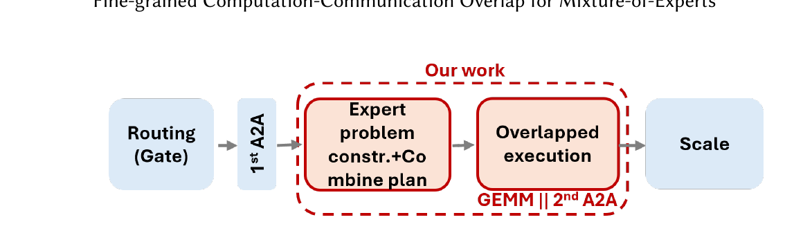
Figure 1 (paper’s own overview diagram, reproduced below) makes the scope explicit: the paper’s contribution (“Our work,” in red) is the box spanning expert-problem-construction-plus-combine-plan and the overlapped GEMM/all-to-all execution. Routing, the first all-to-all, and the final scale step are unmodified — this paper only touches what happens between “tokens have arrived at their expert” and “expert outputs have arrived back home.”

Two phases do the real work, and they map to two subsections of the paper (Section 3.2 and 3.3) that we unpack in detail below:

• Phase A — Expert problem construction and combine plan (a pre-processing / metadata step, no communication yet). Given the routing decisions from the gate, this phase (1) reorders the GEMM’s input rows so that each output tile will belong to exactly one destination rank (the “remote-owner-aligned row layout”), (2) builds a schedule that tells the GEMM which tiles to compute in which order (the “remote-first tile schedule”), and (3) precomputes, for every tile, the metadata a consumer will need to ship it out immediately once it is done (the “combine plan”: destination rank, remote write offset, valid row count).
• Phase B — Overlapped execution (the actual runtime overlap). Two persistent kernels run concurrently: a producer (the rank-wide GEMM, computing expert outputs tile by tile, following the schedule from Phase A, and raising a signal in its epilogue when each tile finishes) and a consumer (a communication kernel occupying a small, disjoint set of SMs, polling the signals and issuing an NVSHMEM put for each completed segment of tiles as soon as it’s ready).

Because the producer processes remote-destined tiles first (by construction of the schedule) and the consumer starts transferring the moment the very first segment of tiles is ready — well before the whole GEMM finishes — the two phases genuinely overlap in wall-clock time rather than merely being pipelined at a coarse batch level.

4. The remote-owner-aligned row layout and tile schedule: derived step by step

This is the mechanistic heart of the paper, so it’s worth working through carefully rather than taking the one-paragraph summary on faith.

4.1 The problem this layout solves

After the first all-to-all, a given local expert e on rank r has received rows (tokens) that originated from potentially every rank in the system — rank 0’s tokens, rank 1’s tokens, rank 2’s tokens, and so on, all mixed together in whatever order the dispatch happened to deliver them. If you naively run the GEMM for expert e on this as-received row ordering, a single output tile (which covers a contiguous chunk of M rows, since GEMM output tiles are tb_M × tb_N rectangles) will, in general, contain rows destined for multiple different owner ranks. That breaks the entire premise of tile-granular overlap: if a tile mixes rows for ranks 0, 2, and 3, the consumer can’t just “ship this tile to rank X” — it would need to inspect every row inside the tile, look up that row’s original owner in some routing metadata table, and issue per-row (not per-tile) transfers. That per-row lookup cost is exactly the overhead the paper is trying to eliminate by working at tile granularity in the first place.

4.2 The fix: reorder rows so tiles are owner-homogeneous

The fix is conceptually simple even though it requires some bookkeeping to implement correctly: reorder the rows before the GEMM runs so that within each local expert’s input, rows are grouped contiguously by their destination (owning) rank, with remote-destined groups first (grouped by which remote rank they belong to) and locally-destined rows last. Concretely, per Section 3.2.1 (Algorithm 1 in the paper), for each local expert e:

1. For every remote rank r' (every rank except the local rank itself), collect the group G_{r'} of rows assigned to expert e whose original owner is r'.
2. If |G_{r'}| is not an exact multiple of the tile height tb_M, pad G_{r'} with zero-filled rows up to the next tb_M-multiple. These padding rows participate in the GEMM’s arithmetic (they don’t need to be skipped mid-computation — a zero-filled row through a linear layer just produces a zero-filled output row, which costs a little wasted compute but changes nothing about correctness) but are excluded from the return transfer — the consumer knows, from the combine plan, exactly how many rows in a segment are “valid” and only ships those.
3. Concatenate all remote groups $G_0, G_1, \ldots$ (skipping the local rank), followed by the local group $G_{r_{\text{self}}}$, to form expert e’s final row ordering X_e.

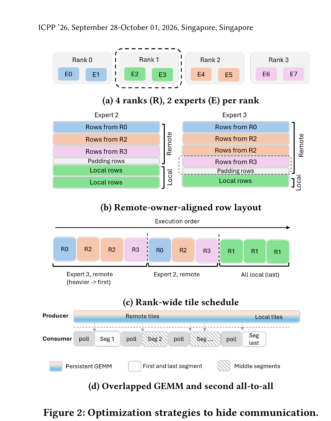
Because padding only ever happens at a group boundary (to round the group up to a tile-height multiple), and because the ordering guarantees remote-rank groups never interleave with each other or with local rows, every full-height output tile now contains rows for exactly one destination rank — the lookup from “which tile” to “which rank does this go to” becomes a single array read rather than a per-row routing decision. Figure 2b (reproduced below) shows this concretely for a 4-rank, 2-experts-per-rank setup: expert 2’s input is laid out as [rows from R0][rows from R2][rows from R3][padding][local rows][local rows], with the padding sitting precisely at the R3-to-local boundary to keep that boundary tile-aligned.

4.3 Why this design, what’s the obvious alternative, and where does it fail

Why this design: it moves all the “which rank does this row belong to” bookkeeping to a one-time, pre-GEMM metadata-construction step (Phase A above), so that during the actual overlapped execution (Phase B), both the producer and the consumer can treat “tile → destination rank” as a flat array lookup with zero per-row branching. This keeps the hot-path kernels — the GEMM main loop and the NVSHMEM transfer loop — free of any conditional routing logic, which matters because conditional branches and scattered memory access patterns are exactly what kill GPU kernel throughput.

The obvious alternative: don’t reorder rows at all; instead, have the consumer kernel inspect each output row’s original-owner metadata at transfer time and issue per-row (or per-small-group) remote writes wherever the owner boundaries happen to fall within a tile. This is architecturally simpler (no upfront row-reordering pass needed) but pays a real, repeated cost: every transfer now requires a lookup into per-row routing metadata, and a tile whose rows straddle two or three owner ranks has to be split into multiple small, potentially non-contiguous remote writes rather than one clean contiguous write. Given the paper’s own measurement (Section 3.3.2 / Figure 3a) that even single-tile transfers (32-64 KiB) sit “far from saturation” on the measured NVLink bandwidth curve, splitting a tile into even smaller per-owner fragments would push transfer sizes further into the low-bandwidth regime — compounding the very problem the paper is trying to solve.

Where the chosen design fails / costs something: the padding is not free. Section 4.5 (Overhead Analysis) works out that the maximum padding per rank is $(W-1)(tb_M - 1)$ rows, where $W$ is the number of ranks — for the paper’s 4-rank setup with tile heights up to 256, that’s up to 765 wasted rows per rank, a genuinely non-trivial fraction (the paper says “a few percent”) of the per-rank row count at the evaluated problem sizes. This overhead is smallest under balanced routing (where group sizes tend to already be near tile-height multiples) and largest under stress_skew routing (where one owner-rank’s row group can be small enough that the padding is a large relative fraction of that group). The paper’s honest conclusion is “the benefits outweigh this cost” — which the throughput numbers in Section 4 do support — but it’s worth flagging that this is a real efficiency tax, not a free lunch, and it scales with the number of ranks, meaning at larger rank counts than the paper’s 4-GPU evaluation, this padding overhead is a real open question (see Section 8, Limitations, below).

4.4 The remote-first tile schedule

Given the row layout above, the paper additionally imposes an execution order on tiles (still Section 3.2.2, Algorithm 1’s second half), governed by two rules:

• Rule (i): all remote-destined tiles are scheduled before any local-only tiles, because only remote tiles require a transfer — local tiles never leave the rank, so there’s no benefit to computing them early.
• Rule (ii): among the local experts on a rank, experts with more remote rows are scheduled first — so the biggest transfers enter the pipeline earliest, maximizing how long the consumer has to drain them before the GEMM as a whole finishes.

Figure 2c shows the resulting schedule for one example rank: expert 3’s remote tiles run first (it has the heavier remote load), then expert 2’s remote tiles, and only then all local tiles (from both experts) at the very end. The intuition, stated in Section 3.2.2, is to “maximize the time window between the first transferable data segment and the end of the GEMM” — the earlier a remote tile is ready, the more slack the consumer has to keep pace with production before the producer runs out of work.

Algorithm 1 (paper’s pseudocode, reproduced with light formatting), the full row-layout + schedule construction:

Require: routing; local rank r_self; rank count R; experts per rank E; tile-M dim tb_M
Ensure: per-expert row layouts {X_e, e in E}; tile schedule S

# --- Remote-owner-aligned Row Layout ---
for each local expert e:
    for each remote rank r' in {0, ..., R-1}, r' != r_self:
        G_{r'} <- rows from rank r' routed to expert e
        if |G_{r'}| mod tb_M != 0:
            pad G_{r'} with zero rows up to the next tb_M-multiple
    append G_0, G_1, ..., G_{R-1} (remote first, G_{r_self} last) to X_e

# --- Remote-first Tile Schedule ---
sort local experts by remote row-band count, descending    # rule (ii)
S <- []
for each expert e in sorted order:
    for each row band b in X_e with destination != r_self:
        append tiles of b to S                              # rule (i): all remote tiles first
for each local expert e:
    for each row band b in X_e with destination == r_self:
        append tiles of b to S
return {X_e, e in E}, S

4.5 The combine plan

To actually ship a completed row band, the consumer needs three pieces of information about it: which rank it’s going to, where in that rank’s receive buffer it should land, and how many rows in it are real (non-padding) data. Resolving these at transfer time by inspecting rows would add per-row overhead to every single transfer — exactly the cost the whole design is trying to avoid. Instead, the “combine plan” (Section 3.2.3) is computed once, up front, by walking the row layout built in step 4.2 and constructing three flat, per-tile, device-resident arrays: destination rank, remote buffer write-offset, and valid-row-count, all indexed by tile identifier. At transfer time, resolving a tile’s destination is then just three array reads — no row inspection, no routing-table lookup, no branching. Every remote-publishable row band gets a single write-offset into its destination rank’s receive buffer, and these offsets are coordinated globally across all local experts so that data from different experts targeting the same peer rank lands at non-overlapping locations in that peer’s buffer.

5. Overlapped execution: producer, consumer, and communication granularity, derived step by step

5.1 The producer: a single rank-wide persistent GEMM kernel

Rather than launching a separate GEMM kernel per expert (which is the conventional pattern, and incurs a kernel-launch overhead for every expert on a rank), the producer is one persistent GEMM kernel per rank, covering all local experts. It’s launched with one persistent CTA per SM; each CTA processes tiles from the schedule S in a strided pattern — CTA i handles tiles i, i+g, i+2g, ... where g is the total CTA (grid) count. For each scheduled tile, a CTA fetches a lightweight “device view” (pointers to that expert’s $A$, $B$, $C$ matrices plus problem-size metadata), copies a shared base parameter block, and overwrites just the expert-varying fields before invoking the actual GEMM tile computation. The paper is careful to note this is a register-level copy, not a kernel re-launch, so switching between experts mid-kernel is essentially free — this is what lets “rank-wide” coverage of multiple experts happen inside a single persistent kernel, distinct from classical “grouped GEMM” which concatenates matrices from multiple problems into one combined problem. Tile-completion signaling is folded directly into the CUTLASS epilogue (following the “Epilogue Visitor Tree,” EVT, pattern the paper cites): after a CTA does its thread-fence to guarantee its finished tile’s data is globally visible in memory, it flips a device-resident readiness flag for that tile — a small, fixed instruction overhead per tile that doesn’t perturb the GEMM’s actual multiply-accumulate main loop.

5.2 Communication granularity: why not just transfer each tile as it finishes?

The naive next step — transfer each tile the instant its readiness flag flips — turns out to be a bad idea, and the paper backs this up with a real bandwidth measurement (Figure 3a, reproduced below). At two example consumer SM budgets (4 and 8 SMs), measured NVLink bandwidth rises steeply with transfer size from small sizes up to roughly 1 MiB, then plateaus (87 GB/s at 8 SMs, 67 GB/s at 4 SMs). A single tile’s payload (32-64 KiB depending on tile configuration) sits far down on the low-bandwidth part of that curve — transferring at single-tile granularity would waste most of the available link bandwidth on protocol/setup overhead relative to payload size.

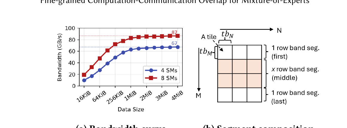
There’s also a structural reason a single tile is a poor transfer unit, independent of bandwidth: a single GEMM output tile only spans tb_N columns out of the full output width N. Even though (by the row-layout construction) a tile’s rows all belong to the same owner rank, the tile’s payload in memory is only a partial-width slice of a full row — meaning it is a strided, non-contiguous memory region if you want to reconstruct the actual output row from it, requiring multiple small copies rather than one clean write. A row band — the full-width strip of tb_M rows spanning all N output columns — is both owner-uniform (same destination rank throughout, by construction) and contiguous in memory, so it can move as a single remote write.

The paper’s resolution (Figure 3b) is a tunable segment partitioning scheme with three cases:

• The first segment is kept to a single row band, so the consumer can issue its very first transfer as soon as humanly possible (minimizing time-to-first-byte).
• The last segment is also kept to a single row band, to avoid a long “communication tail” — a larger final segment would both have to wait longer for its constituent tiles to finish and take longer to transfer once ready, compounding the risk of communication spilling past the end of the GEMM.
• Middle segments coalesce x consecutive row bands, where x (denoted mgb, “multiple of gap bands,” in the paper’s notation) is a tunable parameter chosen so each interior transfer’s payload lands on the saturated part of the bandwidth curve.

The paper is explicit that the optimal x is empirical and workload-dependent — their own evaluation (Section 4) finds neither x=1 (~1-2 MiB) nor x=2 (~2-4 MiB) is uniformly best, because merging more row bands into a bigger interior segment only pays off when the resulting bandwidth gain exceeds the extra wait time it imposes on the consumer before that segment can be issued at all. This is a genuine, unresolved trade-off knob, not something the paper claims to have a closed-form answer for — see the critical-analysis section below for why treating this as a design limitation matters for anyone trying to deploy this in a new setting.

5.3 Producer-consumer co-scheduling: streams, priority, and SM partitioning

The final piece is making sure the two kernels — the GEMM producer and the NVSHMEM consumer — genuinely execute in parallel rather than one starving the other for GPU resources. Three concrete techniques (Section 3.3.3):

1. Separate CUDA streams, asymmetric priority. Both kernels run on independent non-blocking streams, but the consumer is given higher scheduling priority than the producer. The reasoning is asymmetric-cost-based: delaying a producer tile only costs time at the very tail of the GEMM (the GEMM as a whole still has plenty of other tiles to keep computing while one tile’s signal is briefly delayed), whereas delaying a consumer transfer pushes directly onto the communication critical path and — because segments are ordered — compounds into delays for every subsequent segment.
2. SM-level partitioning. Because the consumer runs at higher priority and each kernel is persistent (occupies a fixed CTA/SM footprint for its whole lifetime), the SMs the consumer occupies are effectively reserved for communication for the whole overlapped-execution window, and the remaining SMs are left to the GEMM. This removes SM-level scheduling interference between the two kernels — the GEMM gets a stable SM budget throughout, and the consumer has guaranteed SMs to sustain the bandwidth plateau discussed above, rather than competing dynamically for shared resources.
3. Device-resident coordination only. Once both persistent kernels are launched and resident, all further coordination between them (tile-ready flags, segment dispatch) happens through device memory — no host (CPU) involvement, and no blocking barrier synchronization, on the critical path.

The consumer’s SM budget itself is a tunable (denoted cCTA in the paper, swept from 2 to 24 in the evaluation) with a real trade-off: too few SMs for the consumer and the transfer pipeline falls behind tile production, spilling communication past the end of the GEMM (this is measured explicitly in Section 4.3.4, discussed in Section 6 below); too many SMs taken from the producer and the GEMM itself slows down enough to offset the benefit of overlapping in the first place. The paper’s default, cCTA=14 (out of 108 total SMs on an A100), is chosen empirically from their own sweep, not derived analytically.

6. Design choices worth interrogating: why, what’s the alternative, where does it fail

Beyond the row-layout choice already discussed in Section 4.3, three more design decisions deserve the same why/alternative/boundary treatment.

Separate kernels with device-resident signaling, instead of a single fused kernel. Why: this keeps the GEMM’s CUTLASS-templated main loop essentially untouched (signaling is added only in the epilogue, a natural, low-overhead insertion point) and keeps the communication logic in its own separate, simpler kernel — no custom inter-kernel barrier protocol, no per-target specialization baked into the GEMM itself. Alternative: fusion-based approaches (the paper cites FlashMoE, CCFuser, COMET) weld computation and communication into one kernel, eliminating kernel-launch and stream-switch overhead entirely and potentially achieving even tighter overlap. Where it fails: the paper’s own related-work discussion concedes that fusion “achieve fine-grained overlap, but at the cost of intrusive software complexity and substantial per-target optimization” — i.e., the separate-kernel design trades some theoretically achievable overlap tightness for dramatically simpler, more portable, more maintainable code. Whether that trade is worth it depends entirely on whether you’re optimizing for peak throughput on one fixed hardware/software target (favor fusion) or for a design that’s easier to port across GEMM shapes, router modes, and hardware generations (favor this paper’s approach) — the paper’s own numbers (Section 4.2.1) show it sometimes trails fusion-adjacent frameworks like Megatron-TE on models with small hidden dimensions, which is exactly the regime where fusion’s tighter integration pays off most.

Higher priority for the consumer than the producer. Why: as argued in Section 5.3, a delayed transfer compounds into every downstream segment, while a delayed GEMM tile only costs time at the tail. Alternative: equal priority, or even higher priority for the producer (reasoning: “the GEMM is the expensive part, protect it”). Where it fails: the paper’s own contention study (Section 4.3.4, discussed below) shows the opposite failure mode is what actually bites in practice — starving the consumer of SMs (not priority per se, but raw SM allocation) is what collapses overlap under skewed routing, suggesting that priority alone is not sufficient; SM allocation size matters at least as much, and the paper doesn’t fully disentangle how much of the benefit comes from priority versus from the disjoint SM partition itself.

A fixed, tunable segment size (mgb) rather than an adaptive one. Why: keeps the consumer’s transfer-issuing logic simple — a static parameter chosen once per deployment, no runtime decision-making overhead. Alternative: an adaptive scheme that grows or shrinks segment size at runtime based on observed producer throughput and consumer backlog (the paper explicitly names this as future work: “Production systems could benefit from a runtime-adaptive SM partition selector, which we leave to future work” — and the same logic would apply to segment size). Where it fails: under router skew (stress_skew), a fixed segment size and fixed SM budget together create the contention pathology measured in Section 4.3.4 — a static configuration tuned for balanced routing can become suboptimal or even actively harmful the moment the routing distribution shifts at runtime, which is exactly what happens in production LLM serving where token-to-expert routing patterns are data-dependent and can shift request-to-request.

Padding at owner-rank group boundaries, rather than accepting mixed-owner tiles with per-row dispatch. Already covered in Section 4.3 above, but worth restating in this list for completeness: the trade is upfront, bounded, quantified compute waste (padding) in exchange for eliminating unbounded, per-row branching overhead at transfer time. The paper quantifies the worst case ($(W{-}1)(tb_M{-}1)$ rows per rank) but does not report how this scales qualitatively as $W$ (rank count) grows well beyond the evaluated 4 ranks — a gap flagged again in the Limitations section below.

7. Experimental results, reproduced with commentary

7.1 Setup

All experiments run on a single node with four NVIDIA A100 GPUs (108 SMs, 40 GB HBM each) connected by intra-node NVLink (25 GB/s per lane, 4 lanes per GPU pair, ~100 GB/s one-way ceiling per peer). Software stack: CUDA 12.1, NCCL 2.29.3, PyTorch 2.6.0, CUTLASS 3.9, NVSHMEM 3.6.5. Four baselines: FasterMoE (customized all-to-all, pipelined with expert compute), Megatron with CUTLASS GroupGEMM, Megatron with NVIDIA’s Transformer Engine, and Tutel (adaptive MoE runtime with tunable pipelining and hierarchical 2D all-to-all). Three evaluated model configurations derived from real transformer architectures — M-GPT (MoE only in the 11th of 12 blocks, a sparse-replacement scenario), M-BERT (MoE in blocks 2/5/8/11, evenly spaced), M-Trans-xl (MoE in all 12 blocks, dense replacement) — all with top-k=2 routing over 64 total experts (16 per rank).

7.2 End-to-end and MoE-layer latency on real models

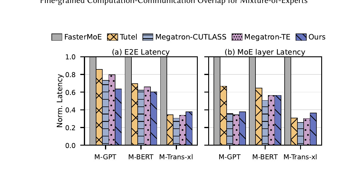
On M-GPT and M-BERT, this paper’s approach consistently beats all four baselines: 1.57x/1.66x over FasterMoE, 1.35x/1.15x over Tutel, 1.15x/1.04x over Megatron-CUTLASS, and 1.25x/1.09x over Megatron-TE (end-to-end); MoE-layer-level gains are larger still (2.65x/1.78x over FasterMoE, 1.77x/1.15x over Tutel). On M-Trans-xl, though, the paper is candid about a genuine weak spot: it beats FasterMoE by 2.64x end-to-end but slightly trails Tutel, Megatron-CUTLASS, and Megatron-TE. The paper’s own explanation is that M-Trans-xl has the smallest hidden dimension (512) of the three models — per-token all-to-all volume scales linearly with hidden dimension, so a smaller dimension leaves less communication to hide in the first place, while the fixed per-tile overhead of fine-grained signaling becomes a larger fraction of an already-shorter layer time. This is a useful, mechanistically-grounded caveat: the technique’s advantage should be expected to shrink (and can even reverse) on models/layers with small hidden dimensions, and a reader deciding whether to adopt this technique should check where their own workload’s hidden-dimension-to-expert-count ratio sits before assuming the headline speedups transfer.

The paper also notes, correctly, that end-to-end speedup is consistently a bit smaller than MoE-layer speedup — by Amdahl’s law, since only the MoE portion of the model is sped up while non-MoE layers (attention, embeddings, etc.) cost the same regardless, the end-to-end gain is bounded by the MoE layer’s share of total model time.

7.3 Scaling with expert count

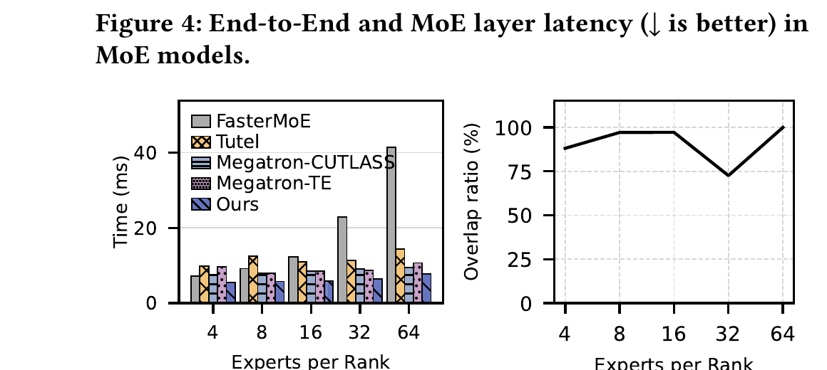
Sweeping experts-per-rank $E$ from 4 to 64 on a single-layer microbenchmark, this paper’s method achieves the lowest layer latency across the entire range, with speedups growing as $E$ grows (1.30x-5.33x over FasterMoE, 1.77x-2.16x over Tutel). This trend makes mechanistic sense: as $E$ grows, both expert compute and return communication scale up together, giving the overlap mechanism proportionally more communication to absorb into the (also-growing) compute time. The overlap-ratio panel is arguably the single most informative result in the paper: the fraction of the second all-to-all successfully hidden behind compute stays between 71.9% and 99.9% across the full sweep, with several configurations approaching full hiding — direct, quantitative confirmation that tile-level signaling exposes communication work early enough for the consumer to keep pace with the producer, rather than merely reducing communication’s exposed cost by some fixed constant factor.

7.4 Operator-level speedup and router skew

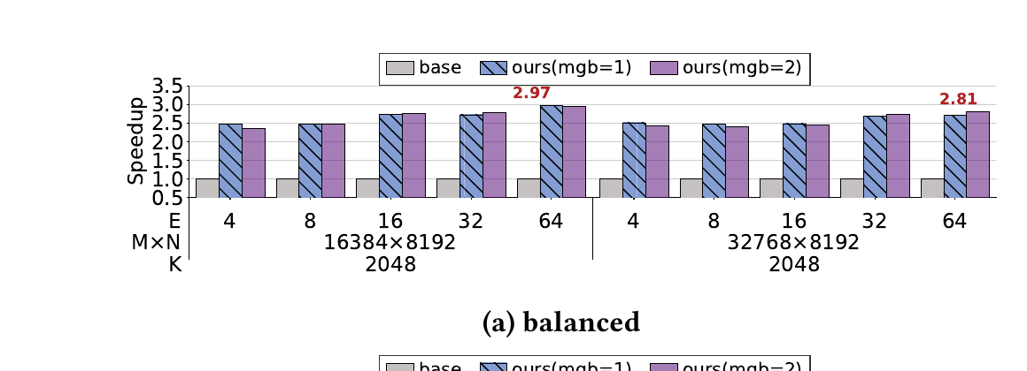
At the pure operator level (isolating just expert-GEMM-plus-second-all-to-all from the rest of the model), speedups over the sequential baseline peak at 2.97x (balanced routing), 2.94x (moderate skew), and 3.01x (stress skew), generally growing with $E$ for the reason given above. Neither mgb=1 nor mgb=2 dominates uniformly across configurations — consistent with the paper’s earlier claim (Section 5.2) that the optimal segment-coalescing factor is workload-dependent, and there is no single best default.

7.5 Resource contention: the SM-partition sensitivity study

Section 4.3.4 of the paper reports a sensitivity sweep over the consumer’s SM allocation (cCTA from 2 to 24, remaining SMs to the GEMM). The headline finding: over-constraining the consumer degrades performance sharply and can make the overlap design actively worse than the non-overlapping sequential baseline. At cCTA=2, the design is slower than the baseline at every tested shape and router mode, reaching 1.91x the baseline’s latency under stress_skew routing at the largest tested problem size — two consumer SMs simply cannot drain completed tiles fast enough, causing back-pressure that collapses the whole overlap benefit. The lowest latency across the sweep is typically achieved with cCTA in the range [10, 20]. Critically, router skew amplifies the contention penalty: the slowdown at cCTA=2 is smallest under balanced routing and largest under stress_skew, because skewed routing concentrates expert-output production onto whichever ranks host the popular experts, and those ranks’ under-provisioned consumers simply cannot keep up with the resulting burst of ready tiles. The paper’s own conclusion here is refreshingly direct: “an effective overlap method must be resource-aware, balancing compute throughput with communication progress rather than maximizing either side in isolation” — and it explicitly flags a runtime-adaptive SM-partition selector as unaddressed future work, rather than papering over the gap.

7.6 Correctness validation

The paper validates correctness across 1,440 independent configuration checks (3 router distributions x 12 SM partitions x 2 mgb values x the shape grid), comparing per-token final output against the sequential baseline with identical seeds, weights, and routing decisions. All checks pass within a relative tolerance of $8 \times 10^{-3}$ except one single iteration on one rank under stress_skew that was not reproducible on rerun (treated, reasonably, as a transient nondeterministic anomaly rather than a correctness bug, given the tolerance level is several times above known FP16 tensor-core rounding noise and far below what a structural bug would produce). The maximum observed relative error across all checks was $1.913 \times 10^{-3}$, roughly an order of magnitude inside the tolerance.

8. Limitations, stated and unstated

Stated by the authors: forward-pass-only (no backward pass / training support — explicitly left to future work); evaluated only on a single 4-GPU intra-node NVLink setup, not at larger scale or across nodes; the SM partition (cCTA) and segment-coalescing factor (mgb) are both static, empirically-tuned parameters rather than adaptive ones, and the authors explicitly flag a runtime-adaptive SM-partition selector as future work; only the second all-to-all (the return/combine path) is overlapped — the first all-to-all (dispatch) is left untouched.

Understated or omitted by the authors:

1. Scaling of the row-padding overhead with rank count is asserted, not measured. Section 4.5 gives a worst-case formula, $(W-1)(tb_M-1)$ padding rows per rank, and evaluates it only at $W=4$. The formula is linear in $W$, which means at, say, $W=32$ or $W=64$ (realistic expert-parallelism degrees for production MoE deployments with hundreds of experts), padding overhead could become a materially larger fraction of total rows — especially combined with skewed routing, where individual owner-rank groups can be small relative to the padding unit. The paper asserts “the benefits of our overlap outweigh this cost” but only demonstrates this at $W=4$; extrapolating that conclusion to larger clusters is exactly the kind of claim the paper doesn’t actually test.

2. No inter-node (cross-NVLink-island) evaluation. All experiments run on a single node with intra-node NVLink, which offers dramatically higher bandwidth (and lower, more predictable latency) than inter-node interconnects (InfiniBand, RoCE, etc.) used when expert-parallelism spans multiple nodes — the realistic deployment regime for the largest production MoE models. The paper’s own bandwidth-curve argument (Figure 3a) for why segment granularity matters is itself NVLink-specific; the optimal segment size, SM partition, and even the basic viability of the overlap-versus-fusion trade-off could look qualitatively different over a slower, higher-latency, more contended inter-node fabric. This is a significant generalization gap that the paper does not address or even flag as future work explicitly (it is implied by “deployment on larger machines” in the conclusion’s future-work list, but not discussed).

3. The cCTA=14 default and the overall “moderate share of SMs, roughly [10,20]” recommendation is derived from a sweep on only two problem shapes (M×N of 16384×8192 and 32768×8192, K=2048), which is a fairly narrow slice of the full workload space defined in the paper’s own Table 2. Whether the same SM-partition sweet spot holds for substantially different GEMM aspect ratios (e.g., very tall-and-narrow or very short-and-wide expert matrices, which do occur in practice with different hidden-dimension-to-expert-count ratios) is not directly tested.

4. The paper compares against four baselines that are all overlap-attempting or communication-optimized systems, but not against the very newest kernel-fusion work it cites in related work (e.g., FlashMoE, COMET, CCFuser) as direct experimental baselines — those are discussed qualitatively in Section 5 (Related Work) but not benchmarked head-to-head in Section 4. Given the paper’s own framing positions itself as a middle path between decomposition-based and fusion-based overlap, the absence of a fusion-based system in the actual speedup comparison (Figures 4-7) leaves an open empirical question about exactly how much overlap-tightness is sacrificed relative to the more invasive fusion approach.

9. Critical analysis

(a) Weaknesses and flaws specific to this paper. The evaluation, while methodologically careful (correctness validated across 1,440 configurations, multiple router-skew regimes, a genuine ablation over SM partition and segment size), is confined to a single hardware generation (A100) and a single node topology (4-GPU intra-node NVLink). Given that the paper’s central motivating claim — GPU compute has outpaced interconnect bandwidth — is itself a claim about hardware trends, and given that the specific numeric bandwidth-saturation point (87 GB/s at 8 SMs, ~1 MiB transfer size, per Figure 3a) is a measured artifact of this specific NVLink generation, it’s a real open question whether the tuned defaults (segment size, SM partition) transfer cleanly to newer interconnects (NVLink 4/5, next-generation NVSHMEM) or to AMD/other accelerator ecosystems, where the bandwidth curve’s shape and saturation point would differ. The paper doesn’t claim portability across hardware generations, but it also doesn’t caveat this limitation explicitly, which a reader evaluating whether to adopt the technique should keep in mind.

(b) Limitations the authors understate or omit. As detailed in Section 8 above, the two most consequential omissions are (i) the lack of any inter-node evaluation, given that large production MoE deployments almost always span multiple nodes with a materially different, higher-latency interconnect than intra-node NVLink, and (ii) the linear-in-rank-count padding overhead formula being validated only at the smallest realistic rank count ($W=4$) tested in the paper, with no data at the rank counts (dozens to low hundreds) actually used by trillion-parameter production MoE systems the paper cites in its own introduction (Switch Transformer, Llama-4-class models). Both gaps matter more, not less, precisely because the paper’s motivating narrative is about scaling MoE to ever-larger deployments.

(c) Concrete, specific improvement suggestions. First, the paper would be substantially strengthened by at least one inter-node experiment — even a 2-node, 8-GPU configuration over InfiniBand would let readers assess whether the tuned segment-size and SM-partition defaults are NVLink-specific artifacts or genuinely more general design principles. Second, given that the authors themselves identify a runtime-adaptive SM-partition selector as important future work, a natural and comparatively low-effort next experiment would be a simple heuristic adaptive controller (e.g., adjusting cCTA based on a running estimate of consumer backlog, using the existing device-resident readiness-flag infrastructure that’s already in place) evaluated against the current static-partition design — this would directly quantify how much of the resource-contention pathology in Section 4.3.4 is recoverable without waiting for a full “future work” cycle. Third, extending the row-padding overhead measurement to at least $W=16$ or $W=32$ ranks (even via a simulated/synthetic routing-distribution experiment, if a real multi-node cluster isn’t available) would let readers directly check whether the “benefits outweigh the cost” conclusion from Section 4.5 still holds at production-realistic expert-parallelism degrees, rather than requiring readers to trust a linear extrapolation from $W=4$.

10. Reproducibility notes

The implementation is described as a CUDA runtime exposed to PyTorch 2.6.0, built on CUDA 12.1, CUTLASS 3.9, and NVSHMEM 3.6.5, with the GEMM built on CUTLASS’s templated kernels using a lookup table of optimal tile configurations derived from the CUTLASS profiler, and tile-level signaling integrated via the CUTLASS epilogue following the EVT (Epilogue Visitor Tree) pattern. The paper does not, in the text reviewed here, state whether the code is or will be released as open source; readers wanting to reproduce the results would need the exact CUTLASS/NVSHMEM/CUDA version combination specified above (version mismatches in NVSHMEM in particular are a known source of subtle behavioral differences in device-initiated communication libraries), the four baseline systems (FasterMoE, Tutel, and Megatron-LM with both the CUTLASS GroupGEMM and Transformer Engine backends) built from their respective public repositories, and access to a multi-A100 node with intra-node NVLink to match the evaluated hardware topology. The correctness-validation protocol (identical seeds/weights/routing across the overlap and baseline paths, comparing final per-token output within a stated FP16-appropriate tolerance) is clearly specified and would be straightforward to replicate as a sanity check on any reimplementation.

11. Where this sits in the broader MoE systems landscape

This paper occupies a specific, well-scoped niche within the broader space of MoE communication-overlap techniques, which the paper’s own related-work section (Section 5) organizes into three families: decomposition-based overlap (chunk the GEMM/collective and pipeline chunks in separate streams — CoCoNet, Centauri, Domino, and MoE-specific pipelining like FasterMoE, PipeMoE, ScheMoE, MPipeMoE), fusion-based overlap (weld computation and communication into one kernel — FlashMoE, COMET, CCFuser), and this paper’s own signaling-based, separate-kernel approach, which the authors position as adopting the “tile-level signaling” principle from prior work (they cite T3 and a paper on “signaling and reordering,” likely referring to work labeled COMET-adjacent or similar in their bibliography) while deliberately keeping compute and communication kernels architecturally separate rather than fused. Relative to this blog’s own prior coverage of MoE and distributed-training systems work — Libra’s attention workload skew handling, Tangram’s GPU-heterogeneity abstraction, and DisagMoE’s disaggregated computation-communication pipeline (still pending publication in this blog’s queue) — this paper sits specifically at the kernel-and-scheduling layer of the MoE systems stack, one level below the disaggregation/placement decisions those other systems make, and is complementary rather than competing with them: a system like DisagMoE decides where (which physical resources) expert compute and communication happen, while this paper’s technique could, in principle, be used to make whatever GEMM/communication step does co-locate on a rank overlap more tightly at the tile level. Readers interested in the fusion-based alternative this paper explicitly declines to pursue should look directly at COMET (cited in this paper’s own related work) for a head-to-head sense of the tighter-overlap-but-more-invasive-engineering trade-off discussed in Section 6 above.

12. Conclusion

This paper’s contribution is narrow but genuinely useful: a way to overlap the second (return) all-to-all of a distributed MoE layer with expert compute at the granularity of individual GEMM output tiles, without resorting to kernel fusion, by solving what turns out to be the actual hard problem — making sure every completed output tile has one clean, unambiguous destination rank — through an upfront row-reordering step (the remote-owner-aligned layout) rather than through invasive per-tile routing logic on the hot path. The engineering is disciplined: tile-completion signaling folds into an existing GEMM epilogue rather than modifying the main loop; the communication kernel is an ordinary, separate persistent kernel using NVSHMEM one-sided writes; and the two kernels are kept from interfering via SM partitioning and stream priority rather than any custom synchronization protocol. The measured results — up to 2.74x MoE-layer speedup, overlap ratios approaching full hiding of the second all-to-all across a wide expert-count sweep, and correctness validated to FP16-rounding-noise tolerance across 1,440 configurations — support the core claim that tile-granular, signaling-based overlap is a practical, non-invasive alternative to both coarse-grained chunked pipelining and full kernel fusion. The honest caveats are equally worth carrying forward: the technique’s benefit shrinks (and can reverse) on small-hidden-dimension models where there’s less communication to hide relative to per-tile signaling overhead; the design is sensitive enough to its SM-partition tuning that a poorly chosen configuration can make things worse than not overlapping at all, especially under skewed routing; and the entire evaluation lives within a single node’s NVLink fabric, leaving the inter-node regime — arguably the regime that matters most for the largest production MoE deployments this paper’s own introduction cites as motivation — untested. For anyone building or tuning distributed MoE inference systems, this paper is a clear, well-documented existence proof that fine-grained overlap is achievable without fusion’s engineering cost; whether its specific tuned parameters transfer to your cluster’s interconnect, rank count, and expert-count regime is the open question this review leaves for you to test.