AnchorKV: Anchor-Residual KV Cache Compression

Review date: 2026-08-05 Author: Zhongzhu Zhou Paper reviewed: AnchorKV: Anchor-Residual KV Cache Compression Paper authors: Malik Khalaf, Yara Shamshoum, Nitzan Hodos, Yuval Sieradzki, Assaf Schuster (Technion — Israel Institute of Technology) arXiv: 2608.02901 Venue/Status: Preprint (cs.LG), August 2026

1. Why this paper, and what problem is it actually solving

Start with a number that should feel uncomfortable if you have ever tried to serve a long-context LLM in production: at 128K tokens, a single Llama-3.1-8B request holds a 16 GiB key-value (KV) cache in bf16 — roughly as large as the model’s own weights. Not the model. The conversation state for one request. Double the context, double the cache. Add concurrent users, and the cache, not the model, decides how many requests a GPU can hold and how fast each one advances. This is the central operational fact that this paper starts from, and it is worth sitting with for a second: in long-context serving, memory bandwidth to fetch the cache at every decode step, and memory capacity to hold it for every concurrent request, are usually the actual bottleneck, not FLOPs.

The field’s answer, broadly, has split into two camps, and the paper’s framing of why neither camp is satisfying is the cleanest part of its motivation.

Camp one: eviction. Score every token in the cache by some importance metric (usually: how much attention it received from a window of “observation queries” near the end of the prompt), keep the highest-scoring subset, and permanently discard the rest. This is the dominant approach in the literature — think SnapKV, PyramidKV, H2O, StreamingLLM’s sink-plus-recency pattern. It is popular because a discarded token costs literally zero bytes, so in principle compression is unbounded: keep 1% of tokens, you get roughly 100x. The catch, which the paper states bluntly and then backs up with hard numbers in Section 4.2, is that the scoring happens before the queries that will actually need the token are known. A token the prompt’s early observation queries ignore might be exactly the token a later decoding query desperately needs — and once it’s evicted, it’s gone. There’s no recovering it. The paper’s own per-task breakdown (their Figure 3, reproduced below) shows this isn’t a rare edge case: on RULER tasks that require retrieving one needle among many distractors or aggregating information scattered across the whole context, eviction baselines collapse to under 16% of the uncompressed accuracy. Not a small regression — a near-total failure on exactly the tasks long-context serving exists to support.

Camp two: quantization. Keep every single token — nothing is ever unreachable — but store each one at lower bit-width (rotation-based INT2/INT4 schemes, per-channel outlier-aware quantizers, and so on). This avoids eviction’s irreversibility entirely. Its problem is depth, not breadth: push the bit-width down far enough to get real compression, and accuracy degrades because every token’s representation is now systematically coarser, not just the unimportant ones. In the paper’s own comparison, the strongest recent quantization baseline (TurboQuant, at a fixed 3.5 bits per value) tracks the uncompressed cache closely but caps out near 5x compression — a full order of magnitude short of where AnchorKV wants to operate.

So you have two families that fail for structurally opposite reasons: eviction is unbounded but brittle (one wrong guess and a needed token is unrecoverable), quantization is safe but shallow (every token pays a uniform quality tax that bounds how far you can push it). AnchorKV’s core idea is to ask: what if you could get eviction’s aggressive compression ratios without eviction’s irreversibility, by never actually removing a token from the softmax, but representing most tokens far more cheaply than a full vector?

The mechanism, previewed in one sentence: pick a small set of tokens per attention head to store exactly (the anchors). Represent every other token as a scaled copy of its closest anchor — literally one integer index and one floating-point scalar, a few bytes instead of a full $D$-dimensional vector. Then take whatever storage budget is left over and spend it on quantized residuals for the specific tokens whose anchor-approximation is estimated to hurt the model’s actual output the most — not the tokens that got the most raw attention, and not the tokens whose residual happens to be numerically largest, but the tokens whose omission would move the final attention output the most. At a 20x compression target, this retains 93–99% of the uncompressed accuracy across three model scales, while every eviction baseline at half that compression ratio (10x) scores lower. If you care about LLM inference cost, long-context serving throughput, or KV cache engineering in general, this paper is a genuinely different point in the design space, not an incremental tweak to either existing family — and the arithmetic behind why it works is worth understanding in detail.

Prerequisites: what you need to know before diving in

If you’re comfortable with self-attention, the KV cache mechanism, RoPE, and the standard vocabulary of KV cache compression (eviction vs. quantization), skip ahead to Section 2. Otherwise, here is the minimum you need.

The KV cache, concretely. During autoregressive decoding, a Transformer must attend every new query token against all previous keys and values. Recomputing keys and values for the whole prefix at every step would be prohibitively expensive, so instead the model caches the key vector $K_t \in \mathbb{R}^D$ and value vector $V_t \in \mathbb{R}^D$ computed for every past position $t$, for every layer, for every attention head. For a sequence of length $S$, $H$ KV heads, head dimension $D$, and $L$ layers, storing everything in bf16 costs $4 \cdot L \cdot H \cdot S \cdot D$ bytes (the factor of 4 comes from 2 bytes each for keys and values). This grows linearly in context length and in the number of concurrent requests a server holds — which is exactly why it becomes the memory bottleneck long before compute does, at long context lengths.

Attention, briefly, in the notation this paper uses. For a single query vector $q$ at decode time, against cached keys $K_1, \ldots, K_S$ and values $V_1, \ldots, V_S$ for one head:

$$s_t = \frac{q^\top K_t}{\sqrt{D}}, \qquad \alpha = \mathrm{softmax}(s), \qquad y = \sum_t \alpha_t V_t.$$

$y$ is the attention output that flows into the rest of the layer. Every KV cache compression method is, at bottom, a way of approximating $K$ and $V$ by some $\hat K, \hat V$ that is cheaper to store, and the entire question of “does this compression method work” reduces to: how far does the reconstructed output $\hat y = \sum_t \hat\alpha_t \hat V_t$ drift from the true $y$?

RoPE (Rotary Position Embeddings). Modern LLMs (Llama, Mistral, Qwen, etc.) don’t add position information to the token embedding; instead they apply a position-dependent rotation $R_t$ directly to the key (and query) vectors before the dot product: the key actually used in attention is $R_t K_t$, not the raw $K_t$ produced by the projection matrix. This detail matters a great deal for AnchorKV, as we’ll see in Section 3 — the paper makes a specific, non-obvious design choice about when in the pipeline to apply its compression relative to this rotation, and gets the wrong choice by a decisive margin if it’s inverted.

Token eviction, as a family. Score every cached position by some importance proxy — most commonly the attention it receives from a small window of the most recent (“observation”) queries, as in SnapKV — and keep only the top-scoring subset up to a token budget, discarding the rest entirely. PyramidKV and AdaKV are refinements that make the budget itself adaptive: PyramidKV varies how many tokens each layer keeps (later layers, empirically, need fewer), AdaKV varies how many tokens each attention head keeps. All three share the same irreversible commitment: once a token is dropped, it can never be recovered, no matter what a later query needs.

KV cache quantization, as a family. Instead of dropping tokens, store every token’s key and value at reduced bit-width — 4-bit, 2-bit, sometimes with a learned rotation (like a Hadamard transform) applied first to spread outlier energy evenly across coordinates before quantizing, which is exactly the trick that makes low-bit quantization tractable at all. TurboQuant, this paper’s quantization baseline, is a recent rotation-based scheme in this family.

Anchors and residuals, the vocabulary this paper needs. An anchor is a token whose key/value vector is stored exactly, with no approximation. A residual is the leftover error vector after approximating some other token as a scaled copy of an anchor — i.e., $r = x - \tilde x$ where $\tilde x$ is the anchor-based approximation of the true vector $x$. Storing a token’s residual (even at low precision) recovers most of what the anchor approximation discarded; not storing it means the token survives only as the scaled anchor copy.

With this vocabulary in place, Section 2 is a direct walk through what AnchorKV builds.

2. Architecture overview: the three-step compression pipeline

AnchorKV runs once, at the end of prefill, on a frozen model — no training, no fine-tuning, no calibration corpus. Given a fixed “retain fraction” $\theta \in (0, 1]$ that the user sets (the single knob that controls compression ratio), each KV head does three things independently, per layer:

1. Select anchors. Pick $k$ positions per head to store exactly: the most recent $W$ positions (a recency window, always kept verbatim) plus a mix of high-attention and randomly sampled earlier positions.
2. Project everything else onto its nearest anchor. Every non-anchor position is represented as a scaled copy of the anchor closest to it in direction, at the cost of one anchor index and one scalar coefficient (a few bytes instead of a full $D$-dimensional vector).
3. Spend a byte-budgeted residual allocation. Whatever storage budget $\theta$ leaves over after paying for the anchors and the projection metadata buys a fixed number of quantized 2-bit residuals, which are handed out — competitively, across all heads in a layer — to the specific tokens whose anchor approximation is estimated to hurt the attention output the most.

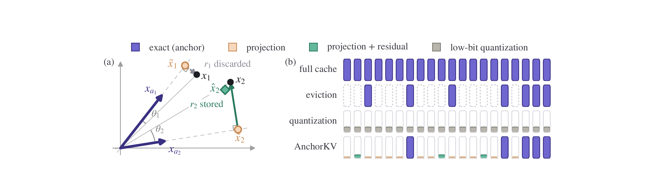
Figure 1 (paper Fig.1): panel (a) shows the representation for two example tokens in $\mathbb{R}^2$. Anchors $x_{a_1}, x_{a_2}$ are stored exactly. Token $x_1$ projects cleanly onto its anchor’s direction and needs no residual ($\hat x_1 = \tilde x_1$). Token $x_2$ projects poorly — the residual $r_2$ it discards is large — so it receives a budgeted 2-bit residual slot, giving the better reconstruction $\hat x_2 = \tilde x_2 + \tilde r_2$. Panel (b) shows why the byte accounting matters: at a matched byte budget, eviction spends everything on a smaller set of exactly-stored tokens, while AnchorKV can afford fewer full anchors precisely because the rest of its budget represents every remaining token at low cost, rather than storing zero information about the tokens it doesn’t keep.

Here is the same pipeline redrawn as a data-flow diagram, separating what happens once at the end of prefill from what happens continuously during decoding:

flowchart TD
    subgraph Prefill["End of prefill (runs once per request)"]
        A["Full K, V tensors for the prompt,
one per layer, per KV head"] --> B["Step 1: Anchor selection
recency window + attention-scored + random"]
        B --> C["Step 2: Assign every non-anchor token
to its nearest anchor by direction (Eq. 1)"]
        C --> D["Compute projection coefficient gamma_i
and residual r_i for every non-anchor token (Eq. 2)"]
        D --> E["Step 3: Score every residual's
attention-output utility (Eq. 6)"]
        E --> F["Byte-budgeted allocation: top-N
residuals by utility get 2-bit slots (Eq. 9)"]
        F --> G["Discard dense K, V.
Store: anchors (bf16) + index/coefficient
per token + sparse quantized residuals"]
    end
    subgraph Decode["Every decode step (repeated per generated token)"]
        H["Fused tiled kernel reconstructs
each key/value tile on the fly"] --> I["Reconstruct: anchor projection
+ residual if stored (Eq. 3)"]
        I --> J["Rotate reconstructed keys by RoPE
(keys were stored pre-RoPE)"]
        J --> K["Standard attention arithmetic;
reconstructed tensors never
written back to memory"]
    end
    G --> H

Two things are worth flagging before the math, because they explain why the design has the shape it has rather than some other shape. First, compression happens exactly once, at the boundary between prefill and decoding — there is no re-optimization as decoding proceeds, and the attention arithmetic itself is completely unchanged; AnchorKV only changes what’s stored and how it’s reconstructed. Second, and this is the sentence that sets up everything that follows: no position ever leaves the softmax. Every token, anchor or not, contributes to every attention computation for the rest of generation. What differs from token to token is how faithfully it’s represented — exactly, via a residual, or only via its anchor projection — never whether it’s present at all. This single design choice is the entire reason AnchorKV can occupy a different point in the compression-vs-accuracy trade-off than eviction: it never pays eviction’s worst-case cost (a needed token that simply isn’t there), because it never removes anything.

3. The anchor-residual representation, derived step by step

3.1 Assignment and projection

Fix a KV head and describe the representation for generic vectors $x_1, \ldots, x_S \in \mathbb{R}^D$ standing for either the keys or the values of that head (the representation is applied to keys and values independently, with separate anchor assignments and separate residual budgets, though both sides share the same anchor positions). A subset $\mathcal{A}$ of the $S$ positions — the anchors — is stored exactly. Every other vector $x_i$ is assigned to whichever anchor’s direction is closest to its own, measured by absolute cosine similarity:

$$a(i) = \arg\max_{a \in \mathcal{A}} \frac{|\langle x_i, x_a\rangle|}{\|x_i\| \|x_a\|}. \tag{1}$$

Why absolute value, not plain cosine? Because what matters for the projection in Eq. 2 below is which direction $x_i$ lies closest to (up to sign) — a token that points nearly opposite to an anchor is still well-represented by that anchor with a negative coefficient, so throwing away the sign at the assignment step doesn’t cost anything and slightly widens the effective anchor coverage.

Having assigned $x_i$ to its anchor $x_{a(i)}$, AnchorKV computes the orthogonal projection of $x_i$ onto the one-dimensional subspace spanned by $x_{a(i)}$:

$$\gamma_i = \frac{\langle x_i, x_{a(i)}\rangle}{\|x_{a(i)}\|^2}, \qquad \tilde x_i = \gamma_i \, x_{a(i)}, \qquad r_i = x_i - \tilde x_i. \tag{2}$$

Unpacking this derivation, because it’s a standard piece of linear algebra worth actually seeing once: the orthogonal projection of a vector $x$ onto the line spanned by a unit vector $u$ is $\langle x, u\rangle u$. Here $x_{a(i)}$ isn’t unit-norm, so we normalize: writing $u = x_{a(i)}/\|x_{a(i)}\|$, the projection is $\langle x_i, u\rangle u = \frac{\langle x_i, x_{a(i)}\rangle}{\|x_{a(i)}\|} \cdot \frac{x_{a(i)}}{\|x_{a(i)}\|} = \frac{\langle x_i, x_{a(i)}\rangle}{\|x_{a(i)}\|^2} x_{a(i)}$ — which is exactly $\gamma_i x_{a(i)}$ with $\gamma_i$ as defined. So $\gamma_i$ is nothing more exotic than “how far along the anchor’s direction does $x_i$ sit,” and because $\gamma_i$ absorbs the anchor’s norm into itself, the anchor and the coefficient together carry the same information a raw dot product would, but packed into a single scalar per token instead of the anchor’s full $D$-dimensional shape being needed again at each token. $r_i$, the residual, is by construction orthogonal to $x_{a(i)}$ — it captures precisely the component of $x_i$ that the anchor’s direction cannot express, no matter how well you scale it.

Finally, the reconstruction rule, which is what actually gets used during decoding:

$$\hat x_i = \tilde x_i + \mathbb{1}[i \in \mathcal{R}]\, \tilde r_i, \tag{3}$$

where $\mathcal{R}$ is whichever subset of positions was granted a stored (quantized) residual $\tilde r_i$ in Section 3.3/3.4 below, and the indicator is zero otherwise. Every non-anchor token is therefore reconstructed from at most three pieces of information: which anchor it belongs to, the scalar $\gamma_i$, and — for the lucky subset in $\mathcal{R}$ — a quantized residual. This is the entire compression mechanism. Anchors need no reconstruction at all ($\hat x_i = x_i$ trivially for $i \in \mathcal{A}$, and the paper implements this uniformly by setting $\gamma_i = 1$ on anchors themselves, so the per-token arrays stay a single uniform shape rather than needing a special case).

3.2 Anchor selection and why keys are projected pre-RoPE

Anchor selection follows the same scoring machinery as SnapKV’s observation window — the paper is explicit that it reuses this exact mechanism, just for a different decision. The final $W$ positions (a small recency window, e.g. $W = 32$ in the experiments) are always kept as anchors; they serve triple duty as the recency buffer, as the “observation queries” whose attention pattern scores the rest of the sequence, and as anchor directions that cost no extra slots beyond what recency already needed. Of the remaining $k - W$ anchor slots, a fraction $\rho$ (0.7 in the paper) goes to the positions with the highest pooled attention score from those observation queries — following SnapKV’s Eq. 14 in Appendix A.2, using average pooling over a small positional kernel so that a sharp attention peak also promotes its neighboring positions, not just the single peak token — and the rest is sampled uniformly at random from the remaining context.

That random component is not an afterthought; it’s solving a real coverage problem. Attention-based selection finds positions the observation queries happen to use directly. But an anchor’s job in this method isn’t just “be an important token” — it’s “provide a good direction for projecting other, unrelated tokens onto.” A token the observation window scored highly is not guaranteed to sit in a direction useful to the many other tokens that will get assigned to it. Uniformly sampled anchors, precisely because they don’t concentrate where attention already concentrates, improve the directional coverage of the anchor dictionary as a whole — the ablation in Section 6 below (component removal, “no random anchors”) measures exactly how much this costs when removed, and the cost is real and grows as the compression ratio tightens.

The pre-RoPE decision deserves its own careful unpacking, because it’s exactly the kind of choice that looks like a minor implementation detail but turns out to move the numbers by a decisive margin (Figure 7, discussed in Section 6.4). RoPE applies a per-position rotation $R_t$ to keys before the attention dot product; crucially, RoPE is a linear map, so it distributes cleanly over the anchor-residual decomposition:

$$R_t K_t = R_t \tilde K_t + R_t r_t^K.$$

This algebraic fact licenses an engineering choice: since the rotation commutes with the sum, AnchorKV can store keys before rotation is applied, and apply the rotation only at decode time, after reconstruction — rather than needing to store a rotation-consistent representation at prefill. But why prefer this, rather than projecting the already-rotated keys? The paper’s argument is that RoPE’s rotation is position-dependent, and two tokens whose un-rotated keys point in very similar directions can end up pointing in quite different directions after each receives its own position-dependent rotation, because the rotation angle itself differs per position. Assigning anchors and computing projections before this position-dependent scrambling is applied means the directional similarity being measured in Eq. 1 reflects the model’s actual semantic content, not an artifact of how far apart two tokens happen to sit in the sequence. Figure 7 (Section 6.4) measures this directly and confirms it: the median cosine similarity between a token and its nearest anchor drops by 0.27 once RoPE is applied — a large, consistent effect across every layer band the paper tested. Since the leftover residual after projection has relative norm $\sqrt{1 - c^2}$ for a cosine similarity $c$ (this follows directly from Pythagoras applied to the orthogonal decomposition in Eq. 2 — if $c$ is the cosine to the anchor, then the projected component has fraction $c$ of the norm and the orthogonal residual has fraction $\sqrt{1-c^2}$), a 0.27 drop in median cosine translates directly into every unrepaired token (i.e., every token that doesn’t get a residual slot) carrying substantially more reconstruction error post-RoPE than pre-RoPE. Fitting before the rotation means the same anchor dictionary covers more of the cache at no extra storage cost — a genuinely free win, once you notice it. Values are unaffected by any of this, since RoPE is only ever applied to keys and queries.

4. Attention-output-aware residual scoring: the mechanism that makes this actually work

Anchors and projections get you some compression, but the paper is explicit that the interesting part — the part that decides whether AnchorKV is competitive with eviction at aggressive ratios — is how the leftover budget (whatever bytes $\theta$ doesn’t spend on anchors and metadata) gets allocated across residuals. Get this wrong, and you’re just a slightly fancier flat quantizer. Get it right, and you concentrate your remaining bytes exactly where they buy the most accuracy.

4.1 Why neither attention score nor residual size is the right ranking criterion

The paper makes a sharp, almost throwaway observation that turns out to be the crux of the whole scoring mechanism: neither the size of a residual nor the raw attention a position receives determines how much storing that residual actually helps. A large residual on a position that barely gets attended to changes the final output very little, no matter how “wrong” the anchor approximation is in isolation. And heavy attention on a position whose anchor already represents it well is also a wasted residual slot — you’d be paying to fix something that wasn’t broken. What you actually want to rank by is each token’s first-order effect on the attention output if its residual were dropped — a quantity that depends on the product of how much attention the token receives and how much error its approximation actually introduces, not either factor alone.

4.2 Deriving the utility score from the softmax Jacobian

Here is the full derivation, because it’s genuinely elegant and the paper compresses it into a few lines that are worth expanding.

Fix a layer, a KV head, and a query $q$. Write the exact logits, attention weights, and output as

$$s_t = \frac{q^\top K_t}{\sqrt{D}}, \qquad \alpha = \mathrm{softmax}(s), \qquad y = \sum_t \alpha_t V_t, \tag{4}$$

and the same quantities computed from the reconstructed cache as $\hat s, \hat\alpha, \hat y$. Compression perturbs $K_t \to K_t + \Delta K_t$ and $V_t \to V_t + \Delta V_t$, and consequently perturbs the logits by $\Delta s_t = q^\top \Delta K_t / \sqrt{D}$.

The key step is a first-order (linearized) expansion of the softmax around the unperturbed logits. The softmax Jacobian is the standard result $\partial \alpha_t / \partial s_u = \alpha_t(\delta_{tu} - \alpha_u)$ (where $\delta_{tu}$ is the Kronecker delta), so to first order in $\Delta s$:

$$\Delta \alpha_t \approx \alpha_t \Delta s_t - \alpha_t \Delta s, \qquad \Delta s = \sum_u \alpha_u \Delta s_u. \tag{5a}$$

This says something worth pausing on: a uniform shift added to every logit changes nothing about the resulting softmax distribution (softmax is shift-invariant), so only the spread of the logit perturbations across positions — how much $\Delta s_t$ differs from the attention-weighted average shift $\Delta s$ — actually matters for how the attention weights move.

Now expand the output perturbation. $\hat y = \sum_t (\alpha_t + \Delta\alpha_t)(V_t + \Delta V_t)$; dropping the second-order cross term $\Delta\alpha_t \Delta V_t$ (this is the linearization, valid when perturbations are small) gives $\Delta y \approx \sum_t \Delta\alpha_t V_t + \sum_t \alpha_t \Delta V_t$. Because $\sum_t \Delta \alpha_t = 0$ exactly (softmax outputs always sum to 1, so any perturbation of one softmax output must be compensated by the others, meaning the $\Delta\alpha_t$ terms themselves sum to zero), you’re free to re-center $V_t$ by subtracting the unperturbed output $y$ from every term in the first sum without changing its value — a small algebraic trick that turns out to matter for the punchline. Substituting Eq. 5a and doing this recentering yields the full result:

$$\Delta y \approx \underbrace{\sum_t \alpha_t \Delta s_t \,(V_t - y)}_{\text{K channel}} \; \underbrace{- \; \Delta s \sum_t \alpha_t (V_t - y)}_{= \, 0} \; + \; \underbrace{\sum_t \alpha_t \Delta V_t}_{\text{V channel}}. \tag{5}$$

(The middle term vanishes because $\sum_t \alpha_t (V_t - y) = y - y = 0$ by definition of $y$ — another consequence of the recentering trick, and the reason the paper phrases Eq. 5 with only two surviving terms despite the derivation passing through three.)

This decomposition is the single most useful sentence in the paper’s theory section: key errors act through the attention weights, and are modulated by how far $V_t$ sits from the output $y$ the query has already formed; value errors act directly and linearly on the output. A key error on a token whose value already agrees with $y$ is nearly harmless — reweighting a token toward or away from an output it would have produced anyway barely moves anything. A key error on a token whose value strongly disagrees with $y$ (i.e., large $\|V_t - y\|$) can meaningfully redirect the output. This is why the two channels get scored by two structurally different formulas below, rather than one shared metric.

4.3 From the perturbation formula to a per-token, additive utility score

Eq. 5 prices the whole cache jointly — it’s a sum over every position’s contribution, all at once. To turn it into something you can use to rank individual tokens for a fixed byte budget, the paper introduces an incoherence approximation: assume, as a working model, that per-token errors are zero-mean and independent across tokens (justified in Appendix A.3 by the fact that the residual codec applies a randomized Hadamard rotation before quantization specifically to spread residual energy across coordinates, making distinct tokens’ residual directions approximately incoherent in high dimension — not a coincidence, but a design choice made partly to support this later approximation). Under this model, cross-terms between distinct tokens vanish in expectation, and the expected squared output perturbation decomposes into a clean sum of additive, per-token terms:

$$\mathbb{E}\|\Delta y\|^2 \approx \sum_t \alpha_t^2\, \mathbb{E}[\Delta s_t^2] \,\|V_t - y\|^2 \; + \; \sum_t \alpha_t^2\, \mathbb{E}\|\Delta V_t\|^2. \tag{5b}$$

The practical payoff of additivity: storing a given token’s residual scales down that token’s term and leaves every other term untouched, and every stored residual costs the same number of bytes (2-bit quantization, fixed dimension). So under this additive approximation, minimizing the total expected squared error for a fixed number of residual slots reduces to “pick the largest terms” — a simple greedy top-$N$ selection is provably optimal for this objective, which is exactly what Section 4.4 below implements.

Now specialize to a token $t$ with no stored residual: its dropped error is exactly its full residual, $\Delta K_t = -R_t r_t^K$ and $\Delta V_t = -r_t^V$ (the negative sign because $\hat x = x + \Delta x$, and reconstructing without the residual removes exactly $r_t$ from the true vector). Plugging into the two terms of Eq. 5b and averaging over the $m = W \cdot (H_q/H)$ observation-window queries of the token’s KV head (in place of an expectation over the queries decoding hasn’t issued yet — a proxy, but the same proxy every observation-window eviction method already relies on), gives the utility of storing token $t$‘s residual on each side:

$$u_t^K = \frac{1}{m} \sum_{w=1}^{m} \alpha_t^{(w)2} \left(\frac{q^{(w)\top} R_t r_t^K}{\sqrt{D}}\right)^{\!2} \left\|V_t - y^{(w)}\right\|^2, \qquad u_t^V = \frac{1}{m} \sum_{w=1}^{m} \alpha_t^{(w)2} \left\|r_t^V\right\|^2. \tag{6}$$

Two things drop out cleanly in this derivation and are worth flagging because they explain why the utility is not just “attention squared” or “residual norm squared” alone: (1) storing a residual replaces the dropped error by the quantization error, whose relative squared energy is $\eta$ (a fixed property of the 2-bit codec, defined precisely in Appendix A.1); since this factor $(1-\eta)$ of recovered energy is common to every token, it cancels out of the ranking — it doesn’t matter for deciding which tokens win the top-$N$ competition, only for the absolute magnitude of the benefit — so it’s dropped from Eq. 6 without loss. (2) Anchors and window tokens are already exact and contribute zero error by construction, so they never even enter this competition; only genuinely approximated, non-anchor, non-window tokens compete for residual slots.

Algorithm 1 below makes the full per-layer pipeline concrete (adapted from the paper’s Algorithm 1, with the residual-allocation step from Section 4.4 folded in explicitly):

Algorithm 1: AnchorKV prefill compression (one layer)
Require: K, V per KV head; window W; anchor budget k; retain fraction θ
 1: for each KV head h do
 2:     A_h ← (last W positions) ∪ (top ρ·(k−W) by SnapKV attention score, Eq.14)
                                   ∪ (remaining slots, sampled uniformly at random)
 3:     for each side ∈ {K, V}:
 4:         for each non-anchor position i:
 5:             a(i) ← arg max_{a in A_h} |<x_i, x_a>| / (||x_i|| ||x_a||)      # Eq. 1
 6:             gamma_i ← <x_i, x_{a(i)}> / ||x_{a(i)}||^2                      # Eq. 2
 7:             x_tilde_i ← gamma_i * x_{a(i)}
 8:             r_i ← x_i - x_tilde_i
 9:         end for
10:         for each non-anchor position i (not in A_h):
11:             u_i ← utility score via Eq. 6 (K-side or V-side formula)
12:         end for
13:     end for
14: end for
15: N ← max(0, floor((θ * M_full − M_base) / b_res))         # Eq. 9, total residual slots
16: N_K ← floor(N/2);  N_V ← N − N_K                         # keys get ⌊N/2⌋, values the rest
17: R_K ← top N_K positions by u^K, POOLED ACROSS ALL HEADS IN THE LAYER
18: R_V ← top N_V positions by u^V, POOLED ACROSS ALL HEADS IN THE LAYER
19: for each side, for each position in R_side:
20:     rotate residual by Hadamard transform U (Eq. 10)
21:     quantize with 4-level Lloyd–Max codebook, 2 bits/coordinate
22:     store packed code + per-token absmax scale
23: end for
24: discard dense K, V tensors

Line 17–18 is easy to skim past but is a real design decision worth naming: residuals are ranked and allocated across all heads in the layer at once, not per head with a fixed per-head quota. This means a head whose tokens are, this particular request, systematically harder to approximate (larger utilities across the board) can claim a larger share of the layer’s total residual budget than a head where anchors already fit well. The ablation in Section 6.2 (“per-head residuals,” i.e., forcing an equal split instead) measures exactly what this pooling buys, and the answer is: real accuracy, and the gap grows as the byte budget tightens, because an equal split literally cannot track which heads need help on a given input.

4.4 Byte-budgeted allocation, worked through with real numbers

The retained fraction $\theta$ (the single user-facing parameter) fixes the total byte budget of a layer. Anchors and per-token bookkeeping metadata are committed first — they are non-negotiable, data-independent costs the moment $k$ and $S$ are fixed — and whatever remains buys residual slots:

$$N = \max\left\{0, \; \left\lfloor \frac{\theta M_{\text{full}} - M_{\text{base}}}{b_{\text{res}}} \right\rfloor \right\}, \tag{9}$$

where $M_{\text{full}} = 4SHD$ is the uncompressed layer size, $M_{\text{base}}$ is the fixed cost of storing the anchors plus every non-anchor token’s index-and-coefficient metadata (Appendix A.1 gives the exact byte accounting, tensor by tensor — anchor keys and values, anchor position IDs, per-token anchor indices, per-token coefficients, a residual bitmask, prefix counts for O(1) lookup, and so on), and $b_{\text{res}}$ is the cost of one quantized residual. This formula is an exact accounting, not an estimate — every byte the decode kernel will actually touch is charged, which is what lets the paper claim the compressed footprint never exceeds the requested budget, unlike some compression schemes whose real memory footprint is fuzzier than the advertised ratio.

The paper’s own worked example (Appendix A.1) is genuinely useful for building intuition: at $S = 32\text{K}$, $D = 128$, $H = 8$, $W = 32$, and anchor budget $k = S/128 = 256$, the uncompressed layer is $M_{\text{full}} = 134.2$ MB. The anchors plus metadata ($M_{\text{base}}$) commit only 3.39 MB — 2.5% of the layer — leaving 3.32 MB of budget at $\theta = 0.05$ (a 20x target) for $N = 91{,}056$ residuals, out of $2HP = 523{,}776$ total token-sides (keys plus values across all non-window positions and heads) that hold some assignment. In other words: at 20x compression, roughly 17% of all token-sides across the layer still get a genuine residual on top of their anchor projection — it is very much not the case that “20x compression” means only 5% of tokens are represented at all; every token is represented, and a meaningful fraction get the extra refinement.

5. Design choices worth interrogating: why, what’s the alternative, where does it fail

Why project each token onto exactly one anchor, rather than a weighted combination of several (like a soft mixture-of-anchors)? The obvious alternative — representing each token as a weighted sum over multiple anchors, the way, say, a learned codebook or product quantizer would — could in principle capture more of a token’s direction than any single anchor can. The paper doesn’t run this ablation directly, but the design rationale is visible in the byte accounting: a single-anchor assignment costs exactly one index and one coefficient, a fixed, tiny, and uniform per-token cost regardless of how well or poorly that assignment fits. A soft multi-anchor scheme would need to store multiple indices and coefficients per token (or a much larger fixed-size sparse/dense weight vector), multiplying the per-token metadata cost and eating directly into the residual budget that Eq. 9 is trying to maximize. Where this single-anchor choice fails: for a token that happens to sit exactly between two anchor directions, no single anchor captures it well, and the entire orthogonal component becomes residual — precisely the situation the paper’s utility scoring (Eq. 6) is designed to detect and prioritize for a residual slot, but if the byte budget is tight enough that this token doesn’t win the top-$N$ competition, it’s stuck with a genuinely bad approximation until compression is relaxed.

Why score residual utility with a first-order (linearized) approximation rather than measuring the true output error directly? The exact, non-approximated attention-output error for every candidate residual assignment would require actually running attention with and without each candidate reconstruction — an operation that’s $O(S)$ per candidate, making exhaustive exact scoring for all $S$ positions cost $O(S^2)$, intractable at the context lengths this method targets (up to 128K). The linearized utility (Eq. 6) is $O(1)$ per token given the cached observation-query attention weights, making the whole scoring pass $O(S)$ total. The cost of linearizing: it’s only valid when perturbations are genuinely “small” in the sense the Taylor expansion assumes, which can break down at extremely aggressive compression ratios where many large residuals are simultaneously dropped and the additive-independence assumption underlying Eq. 5b (that cross-terms between distinct dropped tokens vanish) becomes less accurate. The paper is honest about this being an approximation “under an incoherence model,” not an exact result — Appendix D.1 measures the actual output error the ranking induces (separately from downstream accuracy) specifically to check how much this approximation costs in practice, which is a good methodological habit, though it’s worth noting this only validates the approximation on the models and context lengths tested, not as a universal guarantee.

Why quantize residuals at a fixed 2 bits, with a Hadamard rotation and a Lloyd–Max codebook, rather than adapting bit-width per residual? A per-residual adaptive bit-width (spend more bits on residuals that matter more, fewer on residuals that matter less) sounds like it should strictly dominate a fixed bit-width, since it’s a strictly more expressive allocation space. The paper’s implicit answer, visible in how the byte accounting in Eq. 9 works, is that the residual selection step (deciding which tokens get a residual slot at all, out of $S$ candidates) already performs the adaptive-allocation job that per-residual bit-width would otherwise need to do — a token judged low-utility simply gets zero bits (no residual at all) rather than a few. Given that a binary “some bits or no bits” decision is already doing the heavy lifting, adding a second, continuous bit-width dimension on top adds implementation complexity (variable-length codes complicate the O(1) position-to-slot lookup the storage layout in Appendix A.1 is built around) for a return that the component-removal ablation (Section 6.2, “naive 2-bit,” which strips out just the Hadamard rotation and codebook, not the bit-width itself) suggests is smaller than getting the rotation right: naive 2-bit quantization (no Hadamard, no Lloyd–Max) is the single largest accuracy loss among all four ablated components, and stays roughly constant across compression ratios — because it degrades every stored residual uniformly, rather than changing how many residuals are stored, which is a structurally different (and apparently more costly) kind of damage than a coarser bit-budget would be.

Why is the utility-based residual-ranking metric applied per-side (separate top-$N_K$ for keys, separate top-$N_V$ for values) with a fixed $\lfloor N/2 \rfloor$-vs-remainder split, rather than a single unified ranking across both sides competing for one shared pool? Eq. 5’s own derivation gives the answer directly: key errors and value errors enter the output through structurally different mechanisms — a key error’s effect is modulated by $\|V_t - y\|$ (it only matters if the token’s value actually disagrees with what the query already expects), while a value error acts linearly and directly. Mixing them into one ranking would require converting both onto a shared scale despite this structural asymmetry, and the fixed keys-get-half split is a simple, robust way to sidestep that comparison problem entirely, at the cost of not being able to shift the whole budget toward whichever side happens to matter more for a specific input. The paper doesn’t ablate the 50/50 split itself, which is a reasonable thing to flag as untested: it’s plausible some workloads have systematically more error concentrated on one side, in which case a fixed split leaves some accuracy on the table relative to an input-adaptive split.

6. Results, reproduced with commentary

6.1 Main comparison: AnchorKV against eviction and quantization baselines

The headline experiment (Figure 2) evaluates three instruction-tuned model scales — Llama-3.1-8B, Mistral-Small-3.1-24B, Llama-3.1-70B — against three long-context benchmarks (RULER-32K, RULER-64K, LongBench), at matched byte budgets (not matched token counts — an important methodological point, since it means eviction and AnchorKV are being compared on the metric that actually matters for a memory-constrained server) against SnapKV, PyramidKV, AdaKV, and TurboQuant.

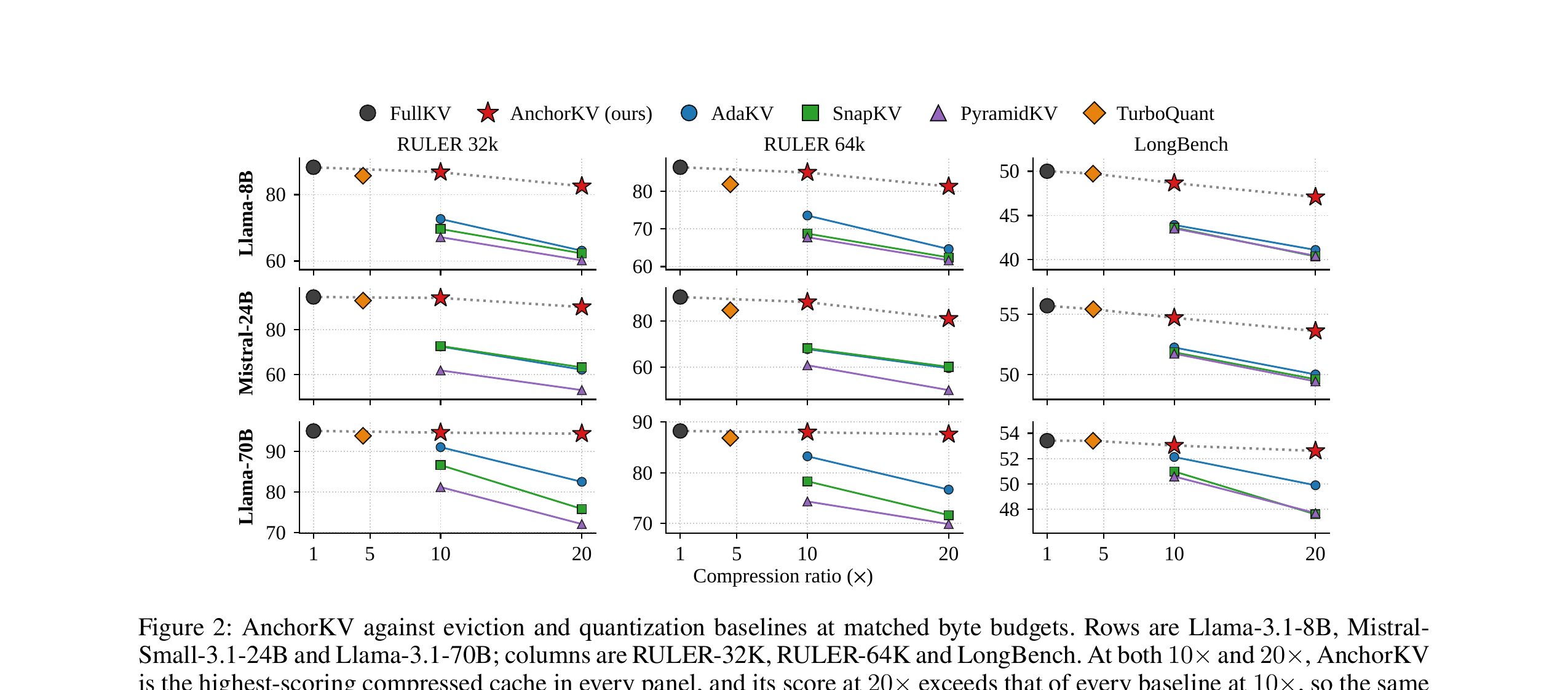
Figure 2 (paper Fig.2): every row is a model scale, every column a benchmark. The pattern is consistent across all nine panels: AnchorKV (red star) tracks the uncompressed FullKV score (black circle, dotted line) closely as compression tightens, while the three eviction baselines (blue/green/purple) degrade sharply — and AnchorKV at 20x consistently sits above where every eviction baseline sits at 10x, meaning the same accuracy is available at half the memory. TurboQuant (orange diamond) tracks FullKV well too, but its fixed 3.5-bit representation caps its reachable compression near 5x — it simply isn’t evaluated in the regime AnchorKV targets, because it structurally can’t get there. Concretely: on RULER-32K at 20x, AnchorKV retains 93.5%, 95.3%, and 99.3% of the FullKV score at 8B, 24B, and 70B respectively, while the strongest eviction baseline at 70B retains only 86.8%.

Two second-order observations the paper draws out are worth restating because they cut against a natural assumption. First, the cost of compression falls with model scale — AnchorKV’s retained accuracy at 20x improves going from 8B to 70B (93.5% → 99.3% on RULER-32K), and this is not simply “bigger models are more robust to any perturbation” in general, because the eviction baselines don’t show the same clean scaling trend (on Mistral-24B, the best eviction baseline stays under 67% at both context lengths — no better than at 8B). Second, LongBench (real documents, less redundancy to exploit than synthetic RULER tasks) shows the same qualitative pattern: AnchorKV retains 94.1% at 8B and 98.4% at 70B, ahead of every baseline at every scale — so the effect isn’t an artifact of RULER’s synthetic structure.

6.2 Per-task breakdown: where eviction actually breaks

Aggregate scores can hide catastrophic per-task failure behind a healthy-looking average, so the paper’s per-task RULER breakdown (Figure 3) is arguably more informative than the headline numbers.

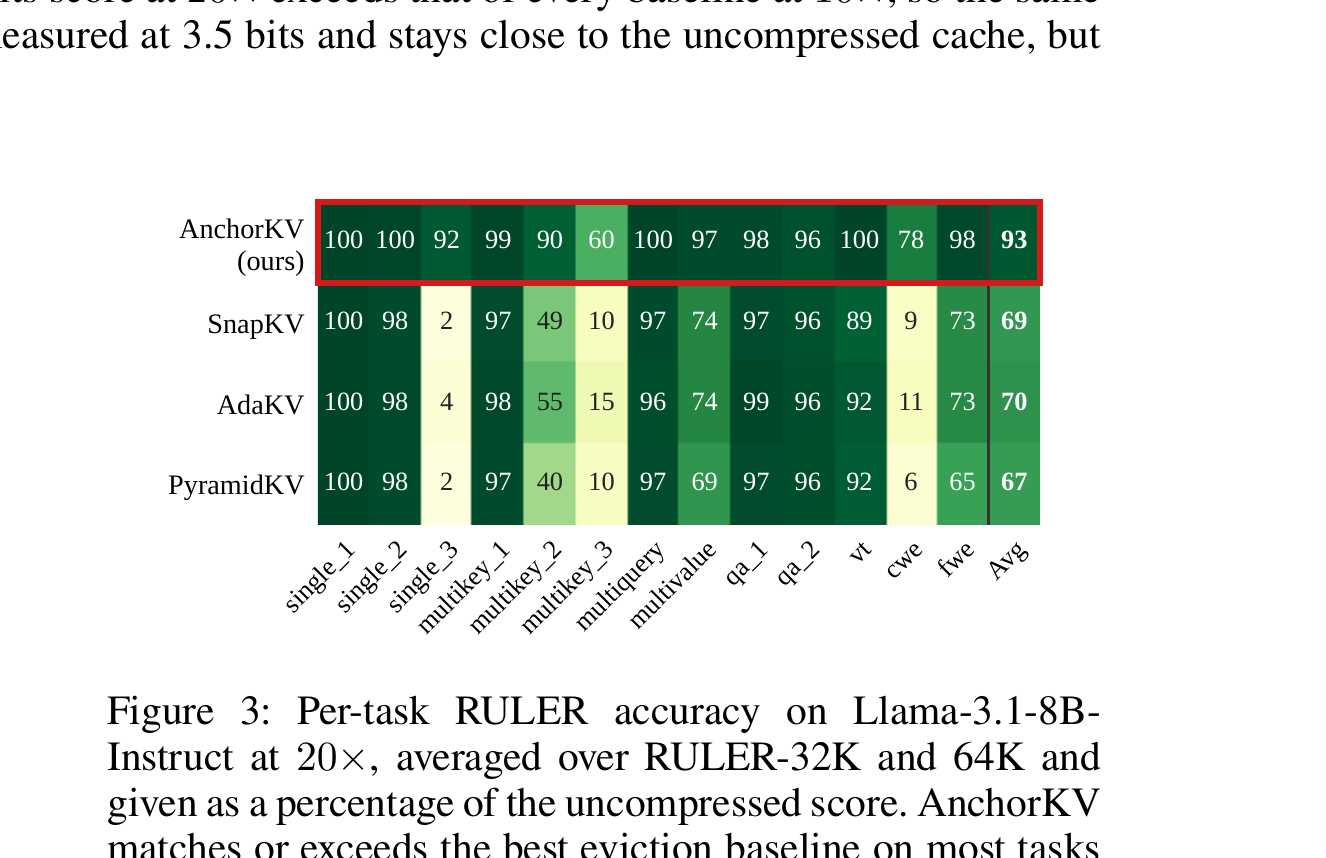
Figure 3 (paper Fig.3): AnchorKV (top row) matches or exceeds the strongest eviction baseline on twelve of thirteen RULER tasks and trails it by a single point on the thirteenth — and its floor across the entire suite never drops below 60%. Contrast this with the eviction baselines: SnapKV, AdaKV, and PyramidKV all collapse to single digits on single_3 (2–4%) and to 40–55% on multikey_2, and PyramidKV drops as low as 6% on cwe. The pattern is exactly what the eviction-brittleness argument from Section 1 predicts: the largest gaps appear precisely on tasks that require retrieval against distractors or aggregation over the whole context — cwe, single_3, multikey_3 — where AnchorKV beats the strongest eviction baseline by 67, 88, and 45 percentage points respectively. These are exactly the tasks where an observation-window scorer, looking only at recent queries, has the least information about what a later query will actually need — and where an irreversible eviction decision is most costly precisely because it can’t be undone.

6.3 A stress test built to break exactly this failure mode

Needle-in-a-haystack retrieval, with a deliberately hard 64-digit passkey (short passkeys, the paper notes, are close to saturated for every method it compares against and wouldn’t distinguish anything), sweeps context length from 16K to 128K and needle depth from 0% (needle at the very start, furthest from the end-of-prompt observation queries) to 100% (needle at the very end, right where the observation window sits).

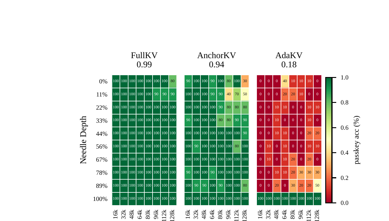
Figure 4 (paper Fig.4): at a comparatively gentle 5x compression ratio, AnchorKV averages 0.94 against 0.99 for the uncompressed cache and recovers the needle across nearly the entire depth-by-length grid. AdaKV, the strongest eviction baseline, averages 0.18 and fails almost everywhere except the very bottom row — and that bottom row isn’t actually a win for AdaKV’s method, it’s an artifact of the benchmark: at 100% needle depth, the needle sits inside the recency window every method (including eviction) stores verbatim, so every method gets it right trivially. The moment the needle moves even slightly away from the end of the prompt, eviction’s observation-window scoring simply never assigns it a high enough score to survive, and it’s gone. AnchorKV’s own weak spots are informative too: its few soft (partially failing) cells cluster at shallow depths in the longest contexts — a needle placed near the very start of a 128K-token prompt is the position furthest, in sequence distance, from the end-of-prompt queries that score anchor candidates, so it’s the position where the anchor-selection heuristic (which reuses SnapKV’s observation-window scoring) has the least direct signal about whether that position will matter later. This is a genuine, acknowledged weak point of the anchor-selection heuristic, not a claim of perfection — it’s just a much smaller failure mode than eviction’s near-total collapse on the same axis.

6.4 Ablations: which design choices are load-bearing

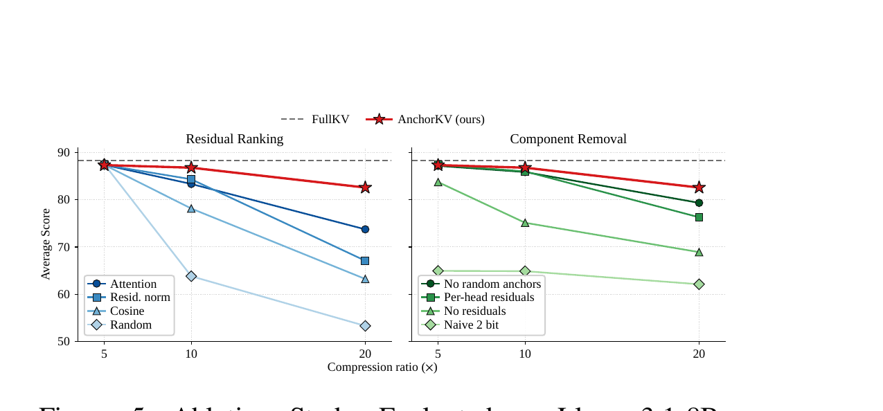
Figure 5 (paper Fig.5), left panel, isolates the effect of the ranking metric used to decide which tokens get a residual, holding anchors and the total budget fixed. In place of the derived utility (Eq. 6), the paper tries ranking by cosine similarity to the nearest anchor (alignment only), by residual norm (approximation error only), by raw attention score (usage only), and by uniform random assignment (a sanity floor). The derived utility wins at every compression ratio tested, and — this is the informative part — at 5x the choice barely matters at all, because the budget is generous enough to reach almost every token regardless of ranking; the gaps only open up as the budget tightens, and are widest at 20x, where random placement falls far behind everything else. The paper’s own explanation for why each single-factor alternative underperforms is worth restating because it maps directly onto the Eq. 5 decomposition: attention score sees how heavily a token is used, but not how badly its anchor represents it; residual norm sees the reverse; cosine similarity sees neither, only the angle. The derived utility is the only metric among the four that combines both factors, which is exactly what Eq. 6’s product of a squared attention term and a squared error term is doing algebraically.

The right panel removes one full component at a time: (i) drop the random anchor share, selecting all anchors by attention score alone; (ii) replace the cross-head pooled residual allocation with an equal, fixed per-head budget; (iii) remove residuals entirely, spending the whole budget on more anchors instead; (iv) quantize residuals naively (2 bits, no Hadamard rotation, no Lloyd–Max codebook). Every removal costs accuracy, but the shape of the cost differs meaningfully: naive quantization is the single largest loss and stays roughly constant across all three ratios tested — a flat tax that doesn’t get worse as compression tightens, because it degrades every stored residual by the same fixed amount regardless of how many are stored. Removing residuals entirely costs accuracy at every ratio even though the freed bytes buy more anchors — a genuinely important negative result, because it directly rules out the tempting simplification “why not just skip the residual complexity and spend the whole budget on more, better-chosen anchors?” A larger anchor dictionary, it turns out, does not substitute for what a targeted residual restores; the two mechanisms aren’t interchangeable, they’re complementary. Equal per-head budgets and attention-only anchor selection cost comparatively little at 5x and progressively more as the budget tightens — the same qualitative pattern the residual-ranking panel shows, which the paper connects to Appendix D.2’s finding that the actual share of residuals different heads need is highly non-uniform and shifts with the specific input, so any fixed equal-split heuristic is structurally unable to track it.

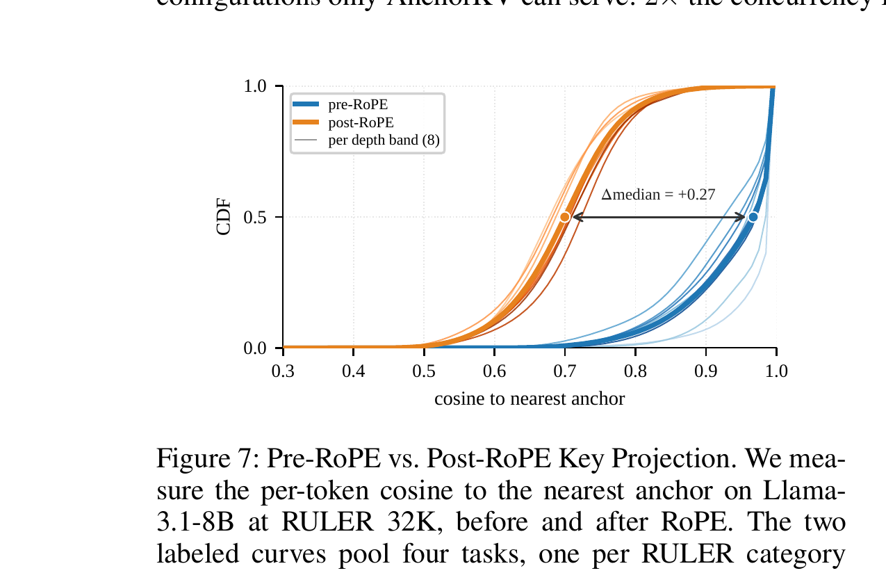
Figure 7 (paper Fig.7) is the empirical confirmation of the pre-RoPE design argument from Section 3.2: the median cosine similarity between a token and its nearest anchor is 0.27 lower when measured after RoPE’s rotation than before it, and this ordering holds consistently across all eight depth bands (groups of consecutive layers) and all four RULER task categories the paper checked — meaning the effect reflects something structural about the rotation itself, not an artifact of one particular layer or task.

6.5 Efficiency: does the accuracy win cost you throughput?

A compression method that preserves accuracy but is too slow to actually use in decoding isn’t a practical win, so the paper profiles a fused Triton kernel that reconstructs keys and values tile-by-tile (FlashAttention-style) directly from the compressed representation, never materializing the dense cache.

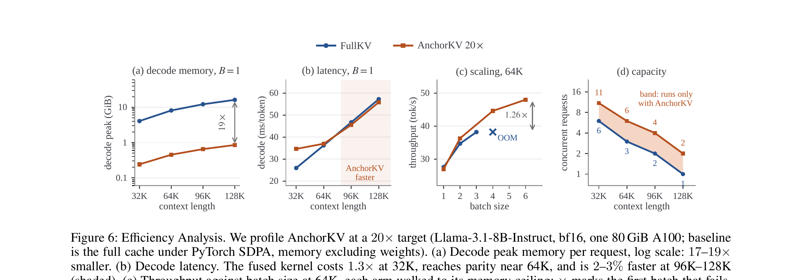
Figure 6 (paper Fig.6): panel (a) shows a 17–19x reduction in steady-state decode peak memory (log scale) — this is the mechanical payoff of never writing reconstructed dense tensors back to global memory; the runtime footprint genuinely is the compressed footprint, not the compressed-footprint-plus-a-temporary-dense-buffer some implementations might need. Panel (b) is the honest part of the story: the fused reconstruction kernel costs roughly 1.3x the decode latency of the uncompressed baseline at short (32K) contexts, where the reconstruction overhead isn’t yet amortized against a large enough per-step workload — but it reaches parity near 64K and becomes 2–3% faster than the uncompressed baseline at 96K–128K, because at long contexts, memory bandwidth to fetch the (much larger) uncompressed cache dominates, and AnchorKV’s smaller footprint wins that bandwidth race even after paying the reconstruction cost. Panels (c) and (d) translate the memory win into what actually matters operationally: at 64K context, AnchorKV sustains a maximum batch size of 6 concurrent requests against 3 for the uncompressed baseline before hitting the memory ceiling — a 1.26x throughput gain when each method is run at its own memory frontier — and the “capacity” panel shows the concurrency gap AnchorKV alone can serve widens further at longer contexts, up to 128K.

7. Limitations, stated and unstated

The paper is reasonably candid about several limitations. All experiments run at batch size 1 on a single A100-80GB; the throughput numbers in Section 6.5 do extend to multi-request batching, but the main accuracy comparisons (Figures 2–5) do not report whether batching interacts with anchor selection or residual allocation in any way (e.g., whether pooling residual budget “across all heads in the layer” behaves differently when many requests share a GPU and compete for the same total memory pool). The method is training-free and calibration-free by design — a genuine strength for deployability — but this also means it cannot learn, across many requests, that certain content types (code, tables, specific languages) are systematically harder to anchor well; every request starts from the same fixed hyperparameters ($W=32$, $k=S/128$, $\rho=0.7$, $\kappa=7$) regardless of what’s actually in the prompt.

The anchor-selection heuristic is explicitly derived from SnapKV’s observation-window scoring, which means it inherits the same fundamental assumption every observation-window method makes: that the positions the last few hundred tokens of the prompt attend to are a good proxy for what future, not-yet-issued decode queries will need. Section 6.3’s needle-in-a-haystack weak spots (shallow depth, longest contexts) are a direct, visible symptom of this assumption’s limits, and the paper is upfront about attributing that specific failure mode to exactly this cause. What the paper does not explore is whether this same assumption degrades further in genuinely multi-turn conversational settings, where “the observation window” at the moment of compression might reflect the first turn’s content and needs, while many subsequent turns’ queries could have systematically different information needs than what the first-turn window could have anticipated — a scenario that is arguably more realistic for production serving than the single-shot long-document benchmarks tested here.

The paper also doesn’t report sensitivity to its own fixed hyperparameters beyond the single reported configuration ($\rho = 0.7$, $\kappa = 7$, $W = 32$) — it’s presented as “one configuration for all models and all tasks,” which is a genuine strength for simplicity and reproducibility, but it leaves open exactly how much accuracy is being left on the table (or, less likely but possible, gained) by not tuning these per model family or per benchmark, and how sensitive the headline numbers actually are to this specific choice.

8. Critical analysis

Weaknesses and flaws specific to this paper. First, the utility-score derivation in Section 4.2–4.3 rests on an incoherence approximation — independence of per-token errors — that the paper justifies partly by design (the Hadamard rotation is chosen specifically to make this assumption more plausible), which is somewhat circular as a validation strategy: the approximation is made more valid by a component whose entire purpose, elsewhere in the pipeline, is to help the quantization codec, and the paper doesn’t independently verify how much the utility ranking’s quality would degrade if that approximation broke down harder — e.g., at compression ratios beyond the 20x tested, where more simultaneously-dropped residuals could plausibly correlate more than the incoherence model assumes. Second, the byte-accounting in Eq. 9 and the worked example in Appendix A.1 charge every stored tensor meticulously, which is commendable rigor — but the comparison against eviction baselines converts eviction’s token-and-bit-width knobs into an equivalent byte budget via a formula ($4BHD$ bytes for $B$ kept tokens) that assumes eviction’s own metadata overhead (position bookkeeping, etc.) is negligible; if eviction methods in practice carry more per-kept-token overhead than this idealized accounting assumes, the “matched byte budget” comparison could be systematically favoring AnchorKV by a small but real margin, and the paper doesn’t discuss this possibility.

Limitations the authors understate or omit. The paper frames the method as fully training-free and hyperparameter-light, which is true relative to methods that require calibration data or fine-tuning — but it undersells how many fixed hyperparameters ($W$, $k$ as a fraction of $S$, $\rho$, $\kappa$, the 2-bit residual precision, the specific 4-level Lloyd–Max codebook) are baked in from a single tuning pass on the models tested, and the paper never demonstrates what happens on a genuinely different architecture family — e.g., a model with grouped-query attention using a much smaller number of KV heads than query heads, where the "$m = W \cdot (H_q/H)$" observation-query count in Eq. 6 could become either very large or very small depending on the specific GQA ratio, with unclear effects on how noisy the utility estimate becomes. Second, all evaluated tasks are read-heavy retrieval/QA/summarization benchmarks; the paper doesn’t test settings with heavy write activity into the cache after compression — e.g., long agentic loops with many tool-call round trips, where newly generated tokens (never compressed, always exact per the method’s design) could eventually dominate an initially-small anchor-selected context, changing the effective compression ratio achieved in practice as generation proceeds, a dynamic the static end-of-prefill compression point doesn’t obviously account for.

Concrete, specific improvement suggestions. (1) Report an ablation on the fixed 50/50 keys-vs-values residual split (Section 5) across at least one workload with a known asymmetric error profile — e.g., a task where key errors are known to dominate (long retrieval chains where softmax renormalization matters a lot) versus one where value errors dominate — to establish whether an input-adaptive split would meaningfully beat the fixed one, rather than leaving this as an implicit, untested design choice. (2) Extend the needle-in-a-haystack stress test (Figure 4) to a genuinely multi-turn setting where the “observation window” used for anchor scoring is taken from an early turn while the needle is injected in a much later turn, directly testing the conversational-drift failure mode flagged in Section 7 rather than only the single-shot version. (3) Provide an explicit sensitivity sweep over at least the two most consequential fixed hyperparameters ($\rho$ and $W$) on one model, holding compression ratio fixed, so readers can judge how much of the headline 20x result depends on this specific tuning versus being robust across a reasonable hyperparameter neighborhood — this is a fairly cheap experiment to add and would substantially strengthen the “one configuration for everything” claim. (4) Directly measure whether the incoherence approximation underlying Eq. 5b degrades gracefully or sharply beyond 20x compression, since the paper’s own framing (“the regime where the cache is most expensive to hold”) suggests practitioners will be tempted to push the method even further than what’s validated here.

9. Reproducibility notes

The paper reports it will release code upon acceptance, and in the meantime documents its experimental setup in unusually granular detail for a systems paper: exact hyperparameters ($W=32$, $k=S/128$, $\rho=0.7$, $\kappa=7$, anchors in bf16, residuals at 2 bits), exact hardware (NVIDIA A100-80GB, batch size 1, greedy decoding, fixed seed 42), and a full byte-accounting table (Appendix A.1, Table 1) precise enough that an independent reader could reimplement the storage layout tensor-by-tensor without guessing. The baselines are run through KVPress, a public library, with documented default settings, which meaningfully reduces the risk of an unfair or miscalibrated baseline comparison — a real and common failure mode in KV-cache-compression papers that compare against reimplemented baselines. RULER, LongBench, and the needle-in-a-haystack setup are all standard, publicly available benchmarks with documented evaluation scripts referenced directly. The one open reproducibility gap, as of this review, is that the actual code (the fused Triton kernel in particular, which is doing real engineering work beyond what’s fully specified in prose) is not yet public, so the efficiency numbers in Section 6.5 cannot currently be independently verified end-to-end, only the accuracy numbers via the documented algorithm and byte accounting.

10. Where this sits in the broader KV cache efficiency landscape

If you’ve been following this blog’s KV cache compression coverage, it’s worth placing AnchorKV explicitly relative to recent work covered here. DynaCalKV (2607.24331, covered in the previous Efficient ML cycle) compresses via head-grouping and adaptive rank allocation — a fundamentally different mechanism (low-rank structure across heads) attacking the same memory bottleneck. LOCKS (2607.24555) and KV-Fold (2605.12471) both pursue compact per-page or recurrent summaries rather than an exact-anchor-plus-residual representation. CounterCausalKV (2607.27600) approaches eviction-style decisions from a counterfactual-surprise angle, still within the “keep a subset, drop the rest” eviction paradigm AnchorKV explicitly contrasts itself against. What makes AnchorKV distinctive relative to all of these is the specific commitment to never removing a position from the softmax while still reaching eviction-competitive compression ratios — it’s less “a better eviction scorer” or “a better quantizer” and more a genuinely third point in the design space, closer in spirit to vector-quantization / codebook methods (which the paper explicitly discusses and differentiates itself from in its Related Work, on the grounds that shared-centroid methods let multiple tokens collapse onto identical representations, while AnchorKV’s per-token scalar coefficient keeps every token distinguishable even when many share an anchor). For a practitioner deciding what to try first on a memory-constrained long-context serving workload, this paper’s own numbers suggest AnchorKV is the strongest available choice specifically when the workload includes tasks with real retrieval-against-distractors or whole-context-aggregation structure — precisely the tasks where eviction’s binary, irreversible commitment is most exposed.

11. Conclusion

AnchorKV’s central bet is that the eviction-vs-quantization dichotomy that has structured most KV cache compression work is a false choice — that you can get eviction’s aggressive compression ratios without paying its irreversibility cost, by never removing a token from the softmax and instead varying how faithfully each token is represented. The mechanics that make this work are genuinely well-motivated end to end: anchors chosen for directional coverage (not just raw importance), a projection whose orthogonal residual captures exactly what the anchor’s direction cannot express, an attention-output-aware utility score derived cleanly from the softmax Jacobian rather than borrowed from a proxy metric, and a byte-exact accounting that turns a single user-facing knob into a provably budget-respecting storage plan. The empirical result — 20x compression at 93–99% of uncompressed accuracy, beating every eviction baseline at half the compression ratio, with the accuracy gap widening in AnchorKV’s favor exactly on the tasks (retrieval-against-distractors, whole-context aggregation) where eviction structurally cannot recover from a wrong early guess — is a genuinely useful data point for anyone deciding how to compress a KV cache in production. The honest caveats (a somewhat circular incoherence approximation, an anchor-selection heuristic that inherits observation-window eviction’s own blind spot to future queries, no code yet released, and untested behavior under multi-turn conversational drift) don’t undercut the core contribution, but they’re exactly the right places to look before assuming the reported 20x number transfers unchanged to a workload meaningfully different from the read-heavy, single-shot long-document benchmarks tested here.