GRPO vs. Dr. GRPO Is Not a Bug-Fix Story: An Impossibility Theorem for Length Bias in Group RL

Review date: 2026-08-04 Review author: Zhongzhu Zhou Paper reviewed: On the Impossibility of Unbiased and Length-Invariant Policy Optimization with Outcome Rewards Paper authors: Fei Ding, Yongkang Zhang, Runhao Liu (Alibaba Group), Yuhao Liao, Zijian Zeng, Huiming Yang (Tsinghua University) arXiv: 2607.23364v1, 2026-07-25 Venue/status: arXiv preprint (cs.LG)

0. Why this paper is worth fifteen minutes of undivided attention

If you’ve trained a reasoning model with RLVR (reinforcement learning with verifiable rewards) in the last two years, you’ve almost certainly hit the following empirical fact: your model’s responses keep getting longer. DeepSeek-R1-Zero’s report flagged it, dozens of open-source reproductions confirmed it, and a 2025 paper called “Understanding R1-Zero-Like Training: A Critical Perspective” (which the community immediately nicknamed Dr. GRPO, for “GRPO, Done Right”) diagnosed a specific mathematical cause inside the standard GRPO objective and proposed a fix: just remove the per-trajectory length normalization term. The claim, more or less verbatim from that paper’s framing, is that doing so produces an unbiased policy-gradient estimator — implying the original GRPO estimator was simply broken, and now it’s fixed.

This new paper — call it the Impossibility paper for short — does something refreshingly precise: it takes that claim at face value, formalizes exactly what “unbiased” and “length-invariant” would have to mean as two separate, well-defined mathematical properties, and then proves — not argues empirically, proves with a short contradiction argument — that no length-based weighting function can have both properties at once. GRPO and Dr. GRPO turn out to be the two endpoints of a continuous, unavoidable one-dimensional tradeoff curve. Calling one of them “done right” doesn’t just overstate the fix; it hides the fact that the fix introduces a different kind of bias, one that is arguably worse in exactly the regime (long, verbose reasoning chains) where these algorithms are used the most.

What makes this paper worth reading closely rather than skimming the abstract: (1) the entire technical contribution is a genuinely short, complete proof you can follow line by line in ten minutes, which is rare in this literature; (2) it comes with sharp, concrete, arithmetic examples (a 10-token correct response vs. a 10,000-token incorrect one) that make the abstract theorem viscerally obvious; and (3) it reframes a full year of “GRPO variant wars” — GRPO, Dr. GRPO, RLOO, REINFORCE++, DAPO’s length-normalization tweaks — as different points on one Pareto frontier rather than a sequence of bug-fixes, which changes how you should read every future paper that claims to have “fixed” GRPO’s length behavior.

If you train LLMs with any group-relative RL objective, or you evaluate papers that tweak how GRPO handles response length, this paper gives you the vocabulary and the proof machinery to see immediately which side of the tradeoff a new method is choosing — and to stop expecting a free lunch.

1. Prerequisites

You don’t need much background beyond basic policy gradients to follow this paper, but it’s worth being crisp about a few pieces of notation and history, because the entire argument hinges on precisely where the “1/L” term in GRPO comes from and what removing it actually changes.

1.1 The token-level language model MDP

Treat autoregressive generation as a Markov Decision Process. Given a prompt $q$, the model samples tokens one at a time: $o_1, o_2, \ldots, o_{|o|}$, where $|o|$ is the response length. At each step $t$, the “state” is the concatenation of prompt and previously generated tokens, $s_t = [q, o_1, \ldots, o_{t-1}]$, and the “action” is the next token $o_t$, drawn from the policy $\pi_\theta(\cdot \mid s_t)$. Generation ends at an end-of-sequence (EOS) token or a length budget.

The RL objective is to maximize expected return:

$$J(\pi_\theta) = \mathbb{E}_{q \sim p_Q}\big[\mathbb{E}_{o \sim \pi_\theta(\cdot \mid q)}[R(q,o)]\big] \tag{1}$$

Outcome reward. In the setting this paper studies — the dominant setting for math/code RLVR — the reward is a single scalar assigned to the entire trajectory after it finishes: $R(q,o) = 1$ if the final answer is correct, $0$ otherwise. Every token in the trajectory shares the same scalar reward; there’s no per-step credit assignment coming from the reward function itself.

1.2 The REINFORCE policy gradient

The vanilla Monte Carlo policy gradient (Williams, 1992) for a trajectory-level return is:

$$\nabla_\theta J(\pi_\theta) = \mathbb{E}_{q,o \sim \pi_\theta}\left[\sum_{t=1}^{|o|} \nabla_\theta \log \pi_\theta(o_t \mid q, o_{<t}) \cdot A(o_t \mid q, o_{<t})\right] \tag{2}$$

where $A(o_t \mid q, o_{<t}) = R(q,o) - B(q, o_{<t})$ is the advantage, and $B$ is any baseline that doesn’t depend on the current action $o_t$ (a classical variance-reduction trick — subtracting a baseline doesn’t change the expectation of the gradient as long as it’s independent of the sampled action). Under outcome reward, since $R(q,o)$ doesn’t depend on $t$, the advantage is the same scalar for every token in a given trajectory.

1.3 Group-relative baselines: where GRPO comes from

Instead of training a separate value network to estimate the baseline $B$ (as PPO does with a critic), GRPO (Shao et al., 2024, from the DeepSeekMath paper) samples $G$ responses $\{o_1, \ldots, o_G\}$ for the same prompt and uses the empirical mean reward across the group as the baseline:

$$\tilde{A}_i = R(q,o_i) - \text{mean}(R) \tag{3}$$

This is elegant because it’s critic-free — no extra network, no value-function training instability — and it’s exactly what made GRPO practical at the scale DeepSeek-R1 was trained at. The full GRPO surrogate objective (omitting the PPO-style clipping term, which the paper notes doesn’t affect this analysis) is:

$$J_{\text{GRPO}}(\theta) = \frac{1}{G}\sum_{i=1}^{G} \frac{1}{|o_i|}\sum_{t=1}^{|o_i|} \frac{\pi_\theta(o_{i,t} \mid q, o_{i,<t})}{\pi_{\theta_{\text{old}}}(o_{i,t} \mid q, o_{i,<t})} \cdot \frac{\tilde{A}_i}{\text{std}(R)} \tag{4}$$

Two normalization terms are baked into this objective: the per-trajectory length normalization $1/|o_i|$ (dividing by the number of tokens before summing) and the group standard-deviation normalization $1/\text{std}(R)$ (used because advantage magnitudes otherwise scale with how “spread out” rewards are within a group). This paper’s analysis is entirely about the first term; it explicitly notes its impossibility result holds regardless of whether the std normalization is used.

1.4 Dr. GRPO’s diagnosis and fix

Liu et al. (2025), the “Understanding R1-Zero-Like Training: A Critical Perspective” paper (nicknamed Dr. GRPO by the community), identified that the $1/|o_i|$ term causes what they call response-level length bias: because every token in a trajectory gets divided by the same $|o_i|$, a long trajectory’s per-token gradient contribution is diluted relative to a short trajectory’s. Their proposed fix is to simply delete both normalization terms:

$$J_{\text{Dr.GRPO}}(\theta) = \frac{1}{G}\sum_{i=1}^{G}\sum_{t=1}^{|o_i|} \frac{\pi_\theta(o_{i,t} \mid q, o_{i,<t})}{\pi_{\theta_{\text{old}}}(o_{i,t} \mid q, o_{i,<t})} \cdot \tilde{A}_i \tag{5}$$

Liu et al. rigorously prove (in their own Appendix A) that Eq. (5)‘s gradient is an unbiased Monte Carlo estimate of the true policy gradient with a group-relative baseline — and, as an aside worth remembering, that this estimator is mathematically equivalent (up to a constant) to REINFORCE Leave-One-Out (RLOO). So this paper’s analysis, as it explicitly notes, also implicates RLOO, even though RLOO is rarely marketed with “length bias” language.

1.5 What this paper adds: a unifying weight function

To compare GRPO and Dr. GRPO (and everything in between) on equal footing, the paper introduces a single weighted-gradient-estimator family parameterized by a length-weighting function $f: \mathbb{N} \to \mathbb{R}^+$:

$$\hat{g}_f = \frac{1}{G}\sum_{i=1}^{G} f(|o_i|) \cdot \tilde{A}_i \cdot \sum_{t=1}^{|o_i|} \nabla_\theta \log \pi_\theta(o_{i,t} \mid q, o_{i,<t}) \tag{6}$$

GRPO is the special case $f(L) = 1/L$; Dr. GRPO is $f(L) = 1$ (both omitting the std(R) factor, since that’s a question-level scalar orthogonal to the length-bias question). Everything the paper proves is a statement about this one-parameter family of functions $f$.

2. Architecture / Pipeline Overview

There’s no neural architecture novelty in this paper — the contribution is entirely mathematical — but it’s useful to see where the theorem sits inside the standard RLVR training loop, and how the two properties (P1, P2) map onto observable training pathologies.

flowchart TD
    A["Prompt q sampled from dataset"] --> B["Sample G responses<br/>o_1 ... o_G from policy π_θ"]
    B --> C["Score each response:<br/>R(q, o_i) = 1 correct / 0 incorrect"]
    C --> D["Group-relative baseline:<br/>Ã_i = R_i - mean(R)"]
    D --> E{"Apply length weight f(L_i)"}
    E -->|"f(L) = 1/L → GRPO"| F["Gradient share independent<br/>of length (P2 holds)<br/>but estimator is biased (P1 fails)"]
    E -->|"f(L) = 1 → Dr. GRPO"| G["Gradient unbiased<br/>(P1 holds)<br/>but longer trajectories dominate<br/>gradient share (P2 fails)"]
    F --> H["Observed pathology:<br/>model biased toward<br/>long wrong answers"]
    G --> I["Observed pathology:<br/>both correct & incorrect<br/>responses drift longer"]
    H --> J["Theorem 6:<br/>no f(L) escapes this tradeoff"]
    I --> J

Figure A (self-drawn): the two failure modes of the two named algorithms are not independent bugs — they are the two visible symptoms of one underlying impossibility.

The key conceptual move the paper makes is separating “is the gradient estimator correct in expectation” (a statistical property, P1) from “does a trajectory’s length affect how much it’s allowed to move the parameters” (a training-dynamics property, P2). These sound like they should both just be “yes” for a well-designed algorithm — that’s exactly the intuition Dr. GRPO’s framing trades on — but the proof shows they’re structurally in tension.

3. Core Theory: Two Properties, Fully Unpacked

3.1 Formal definitions (Definitions 4 and 5 in the paper)

Definition 4 (Trajectory-level correctness, P1). The estimator $\hat{g}_f$ satisfies P1 over a policy class $\Pi$ if there’s a constant $c > 0$, independent of the trajectory-length distribution, such that for every policy $\pi \in \Pi$:

$$\mathbb{E}_\pi[\hat{g}_f] = c\, \nabla_\theta J(\pi) \tag{11}$$

In plain language: whatever length distribution the current policy happens to produce, the expected gradient still points in (a fixed positive rescaling of) the true policy-gradient direction. This is what “unbiased” is supposed to mean.

Definition 5 (Length neutrality, P2). Define $\Gamma_{\pi,\rho}(L; a) := \mathbb{E}_\pi[\rho(S) \mid L(\tau)=L, \tilde{A}(\tau)=a]$ — the expected magnitude (under some scale functional $\rho$, e.g. a vector norm) of the per-trajectory score-sum $S = \sum_t \nabla_\theta \log \pi_\theta(o_t \mid q, o_{<t})$, conditioned on a fixed trajectory length $L$ and a fixed realized advantage $a$. The estimator satisfies P2 if:

$$f(L)\, \Gamma_{\pi,\rho}(L; a) \tag{13}$$

is the same number regardless of which realizable length $L$ you plug in (holding the advantage $a$ fixed). In plain language: two trajectories that get the same reward signal (both correct, say) should contribute the same amount to the gradient update, whether one is 200 tokens and the other is 6,000 tokens. Length shouldn’t be a hidden lever on how much a trajectory gets reinforced.

Both of these are reasonable, independently desirable things to want. The theorem’s punch line is that you cannot have both, for any choice of $f$ depending only on length.

3.2 Theorem 6, step by step

Setup. Fix a weight function $f: \mathbb{N} \to \mathbb{R}^+$. Assume (Assumption 2, “fixed-length realizability”) that for some set of realizable lengths $\mathcal{L}$, the policy class actually contains policies that produce a fixed length $L$ almost surely while still having non-degenerate randomness in the content of the tokens — this is a technical condition needed so we can talk about “the same length, different possible advantages” without the length itself being forced by content. Assume also (Assumption 3) the scale functional $\rho$ is positively homogeneous of degree one (true of any norm).

Claim. If there exist a policy $\pi^\star$, an advantage value $a^\star$, and two distinct realizable lengths $L_1 \neq L_2$ such that $\Gamma_{\pi^\star,\rho}(L_1;a^\star) \neq \Gamma_{\pi^\star,\rho}(L_2;a^\star)$ (i.e., the “typical size” of the score-sum really does depend on length, which is true whenever response-length variance is non-negligible), then no $f$ can satisfy both P1 and P2.

Proof, unpacked in full:

Step 1 — P1 forces $f$ to be constant. Pick any realizable length $L_0 \in \mathcal{L}$. Under the fixed-length policy $\pi^{(L_0)}$ (all trajectories have length exactly $L_0$), all $L_i = L_0$, so the estimator collapses to:

$$\hat{g}_f = f(L_0) \cdot \frac{1}{G}\sum_{i=1}^{G} \tilde{A}_i S_i \tag{16}$$

Expand the group-relative baseline $\tilde{A}_i = R_i - \text{mean}(R) = \left(1 - \frac{1}{G}\right) R_i - \frac{1}{G}\sum_{j \neq i} R_j$ and take the expectation. Because within-group trajectories are conditionally i.i.d. given the prompt, $R_j$ (for $j \neq i$) is independent of $S_i$, and by the score-function identity $\mathbb{E}_{\pi^{(L_0)}}[S_i] = 0$ (this is the standard fact that $\mathbb{E}_\pi[\nabla_\theta \log \pi_\theta(o)] = 0$, since $\nabla_\theta \sum_o \pi_\theta(o) = \nabla_\theta 1 = 0$). So all the cross terms $\mathbb{E}[R_j S_i] = \mathbb{E}[R_j]\mathbb{E}[S_i] = 0$ vanish, leaving:

$$\mathbb{E}_{\pi^{(L_0)}}[\tilde{A}_i S_i] = \left(1 - \frac{1}{G}\right) \mathbb{E}_{\pi^{(L_0)}}[R_i S_i] = \left(1 - \frac{1}{G}\right) \nabla_\theta J(\pi^{(L_0)}) \tag{21-22}$$

using the REINFORCE identity $\mathbb{E}[R_i S_i] = \nabla_\theta J$. Substituting back:

$$\mathbb{E}_{\pi^{(L_0)}}[\hat{g}_f] = f(L_0) \cdot \frac{G-1}{G} \cdot \nabla_\theta J(\pi^{(L_0)}) \tag{23}$$

If P1 holds, this must equal $c \cdot \nabla_\theta J(\pi^{(L_0)})$ for a length-independent constant $c$, so $f(L_0) \cdot \frac{G-1}{G} = c$ for every $L_0 \in \mathcal{L}$ — which forces $f$ to be literally constant, $f(L) \equiv c_0$, across all realizable lengths.

Step 2 — P2 forces $f$ to be non-constant. Suppose for contradiction $f \equiv c_0$. Substituting into the P2 condition $f(L)\Gamma_{\pi,\rho}(L;a) = C_{\pi,a}$ (a constant independent of $L$) at $\pi = \pi^\star, a = a^\star$ gives $c_0 \Gamma_{\pi^\star,\rho}(L_1;a^\star) = c_0 \Gamma_{\pi^\star,\rho}(L_2;a^\star)$. Since $c_0 > 0$, this implies $\Gamma_{\pi^\star,\rho}(L_1;a^\star) = \Gamma_{\pi^\star,\rho}(L_2;a^\star)$ — directly contradicting the assumption that these two quantities differ.

Step 3 — contradiction. Step 1 says: if P1 holds, $f$ must be constant. Step 2 says: if $f$ is constant, P2 fails (given the non-trivial length-dependence assumption). So P1 and P2 cannot both hold. $\blacksquare$

Intuition, once you strip the algebra away. P1 says “a uniform length-weighting doesn’t distort the original trajectory-level policy-gradient objective” — which mathematically requires the weight $f$ to not vary with length (any variation would introduce a length-dependent rescaling that breaks the unbiasedness identity). P2 says “the weight should vary with length, specifically to cancel out the fact that longer trajectories naturally accumulate bigger score-sums (more terms in the $\sum_t \nabla \log \pi_\theta$ sum).” One property demands constancy; the other demands non-constancy, precisely because it’s designed to compensate for something that scales with length. There’s no way to thread that needle with a single scalar function of length alone.

Scope, honestly stated. The theorem only rules out weight functions depending solely on length. It leaves the door open for schemes that condition on token position, local context, score geometry, or finer-grained credit assignment — the paper is explicit that this is future work, not something it’s already ruled out.

3.3 Algorithm view: how you’d actually check where your training run sits on the tradeoff

The paper doesn’t present this as literal pseudocode, but it’s useful to make the “diagnostic” implicit in the theorem concrete and executable, since that’s what you’d actually run against a training log:

Algorithm 1: Diagnosing which side of the P1/P2 tradeoff your RL run is on
Input: batch of (prompt, group of G responses, rewards, lengths)
Output: empirical bias estimates for P1 violation and P2 violation

1:  for each training step do
2:      collect {(o_i, R_i, L_i)}_{i=1}^{G} for the current prompt group
3:      compute Ã_i = R_i - mean(R)                          # Eq. 3
4:      compute per-trajectory score sum S_i = Σ_t ∇_θ log π_θ(o_{i,t} | ·)
5:      # --- P1 empirical check: gradient-bias term (Corollary 12) ---
6:      compute bias_P1 ≈ (1/G) Σ_i Ã_i (f(L_i) - c̄) · S_i     # non-zero iff L_i correlates with S_i
7:      # --- P2 empirical check: length-weight share (Corollary 9) ---
8:      compute w_i = f(L_i) |S_i| |Ã_i| / Σ_j f(L_j) |S_j| |Ã_j|
9:      flag "P2 violated at this step" if max_i w_i - min_i w_i exceeds tolerance ε
10: end for
11: aggregate bias_P1 and the w_i spread over the run
12: report: which regime (GRPO-like / Dr.GRPO-like / intermediate α) the run's
    empirical (bias_P1, length-weight spread) pair is closest to on the Pareto curve

Worked toy example, to make Algorithm 1 concrete. Take $G=2$, one correct trajectory $o_1$ ($R_1=1$, $L_1=10$ tokens) and one incorrect $o_2$ ($R_2=0$, $L_2=10{,}000$ tokens) — this is Example 10 from the paper. The advantages are $\tilde{A}_1 = +0.5$, $\tilde{A}_2 = -0.5$. Under Dr. GRPO ($f\equiv 1$), the gradient-contribution magnitudes are $10 \times 0.5 = 5$ for $o_1$ and $10{,}000 \times 0.5 = 5{,}000$ for $o_2$ — the incorrect, verbose trajectory captures $5000/5005 \approx 99.9\%$ of the total gradient magnitude, meaning the “run step 8” weight-spread check in Algorithm 1 would flag this instantly ($w_{o_2} - w_{o_1} \approx 0.998 \gg \varepsilon$). Under GRPO ($f(L)=1/L$), both contribute exactly $0.5 \times 1 = 0.5$ regardless of length — no spread, P2 holds locally, but (per Corollary 12 below) there’s now a systematic bias correlated with whichever tokens tend to co-occur with short vs. long responses.

4. Design Choices, Unpacked

Choice 1 — Why compare against a parametric family $f_\alpha(L) = L^{\alpha-1}$ rather than just two isolated algorithms? Why it works: framing GRPO ($\alpha=0$) and Dr. GRPO ($\alpha=1$) as endpoints of a continuum immediately tells you there’s a dial, not a binary choice, and that intermediate values ($\alpha \in (0,1)$) trade off partial bias for partial length-sensitivity in a quantifiable, monotone way (Corollary 8: bias $\propto |\alpha - 1|$, length bias $\propto \alpha$). The obvious alternative — just benchmark GRPO vs. Dr. GRPO empirically on a handful of tasks, as most papers in this space do — tells you which one wins on your benchmark, but not why, and gives you no lever to interpolate when neither endpoint is right for your setting. Where the parametric framing is weaker: the paper doesn’t derive or recommend an optimal $\alpha^*$ as a function of measurable training statistics (e.g. observed length variance); it stops at “practical guidance” heuristics (Section 4, see below), leaving the actual dial-setting as an empirical exercise for the practitioner.

Choice 2 — Why the “fixed-length realizability” assumption (Assumption 2) instead of proving the theorem unconditionally over arbitrary policies? Why it works: this assumption is what lets the proof isolate pure length effects from confounded effects (e.g., a policy where length and correctness are entangled in a complicated way). By constructing a hypothetical policy that produces a fixed length almost surely while still having random content, the proof can cleanly compute $\mathbb{E}[\hat g_f]$ under that policy and derive a length-indexed constraint on $f$. The obvious alternative — proving it directly for the actual trained policy’s length distribution — would be much harder to state cleanly and would conflate “this specific model’s” length/correctness correlation with the structural impossibility the paper wants to establish, which is a property of the estimator family, not any one policy. Where it’s a real limitation: real trained policies are never exactly fixed-length; the theorem’s guarantee is about what’s mathematically achievable in principle across the policy class, and its practical bite depends on how close a real training run’s length variance gets to violating the non-triviality condition (which the paper argues is essentially always, in reasoning tasks with variable-length outputs).

Choice 3 — Why binary outcome reward (0/1 correctness) rather than richer, continuous reward shaping in the corollaries’ worked examples? Why it works: binary outcome reward is the setting used by essentially every RLVR reasoning pipeline (DeepSeek-R1-Zero, Open-Reasoner-Zero, etc.), so grounding the quantitative corollaries (Corollary 9, 12, 13) here maximizes real-world relevance and lets the paper cite an actual empirical number from DeepSeek-R1-Zero’s training log (Example 11: 4,965 vs. 8,206 average tokens) to anchor the abstract theorem in a concrete, already-observed 62.3% gradient share. The alternative — deriving the corollaries for continuous process rewards or reward models — is explicitly flagged by the authors (in Limitations) as future work, and is genuinely harder because the advantage is no longer constant across tokens in a trajectory, so the clean $|o_i| \cdot \tilde A_i$ factorization used throughout Section 4 breaks down.

Choice 4 — Why frame the paper as a rebuttal of a specific prior claim (“Dr. GRPO / GRPO Done Right”) rather than a standalone impossibility result? Why it works: anchoring against a widely-cited, widely-adopted specific claim gives the result immediate practical stakes — it’s not “here’s an abstract fact about weight functions,” it’s “the algorithm many of you switched to because it was called ‘done right’ has its own, differently-shaped bias, and neither name is accurate.” This framing is also honest about crediting Dr. GRPO’s correct half of the claim (the gradient-unbiasedness proof genuinely holds, as re-verified here) while contesting only the completeness of the “done right” framing. The risk of this framing choice: it can read as adversarial toward a specific, recent, well-regarded paper, and a reader skimming only the title might mistake this for “Dr. GRPO is wrong” rather than the more nuanced (and correct) claim that Dr. GRPO makes a legitimate but under-advertised tradeoff.

4.5 A worked comparison: mapping known GRPO variants onto the tradeoff curve

One of the most useful exercises this paper enables — even though it doesn’t do this itself — is placing every GRPO variant you’ve heard of onto the $\alpha \in [0,1]$ axis and asking which side of the tradeoff it’s really choosing. Here’s my own attempt at that audit, which is exactly the kind of table I wished the paper had included:

Method	Effective length weighting	P1 (unbiased)	P2 (length-invariant)	Practical symptom
GRPO (Shao et al. 2024)	$f(L)=1/L$	✗ (biased, Corollary 12)	~✓ (equal weight regardless of length)	biased toward long wrong answers
Dr. GRPO / RLOO (Liu et al. 2025; Kool et al. 2019)	$f(L)=1$	✓	✗ (Corollary 9: longer traj. dominates)	both correct & incorrect responses drift longer
DAPO’s token-level loss aggregation	closer to $f(L)=1$ at the batch level	✓-leaning	✗-leaning	similar length-growth pressure to Dr. GRPO, mitigated by other DAPO components (clip-higher, dynamic sampling)
GSPO’s sequence-level importance ratio	conceptually closer to $\alpha \approx 1$ but reweights the ratio, not just the gradient sum	partial	partial	different mechanism entirely — worth a dedicated re-analysis, not covered by this paper
Intermediate $\alpha \in (0,1)$ schemes (not yet named/adopted widely)	$f_\alpha(L)=L^{\alpha-1}$	partial	partial	untested in the literature at scale as of this paper’s writing

The columns for DAPO and GSPO are my own extrapolation, not claims made in the paper — the point of building this table is to show how immediately actionable the paper’s framework becomes once you start asking “where does variant X actually sit” rather than treating the theorem as a purely abstract fact.

4.6 Why the choice of $\rho$ (the scale functional) matters less than it looks

A question a careful reader will have: Definition 5’s length-neutrality property is stated relative to an arbitrary scale functional $\rho$ (e.g., a vector norm). Does the impossibility result depend sensitively on which $\rho$ you pick? The proof’s Step 2 only uses that $\rho$ is positively homogeneous of degree one (Assumption 3) — a very weak requirement satisfied by essentially every reasonable notion of “gradient magnitude” (any norm, or even a signed projection onto a fixed direction as the paper notes). This robustness is a genuine strength: the impossibility isn’t an artifact of some idiosyncratic choice of how you measure gradient size, it holds for the entire natural class of magnitude measures.

flowchart LR
    subgraph Legend["Reading the tradeoff axis"]
        direction TB
        L0["α = 0 (GRPO)<br/>f(L) = 1/L"] --> L05["α = 0.5<br/>f(L) = L^-0.5"]
        L05 --> L1["α = 1 (Dr. GRPO)<br/>f(L) = 1"]
    end
    L0 -.->|"gradient bias ∝ |α-1|"| Bias["Bias axis:<br/>high at α=0,<br/>zero at α=1"]
    L1 -.->|"length bias ∝ α"| Len["Length-bias axis:<br/>zero at α=0,<br/>high at α=1"]

Figure B (self-drawn): the two error sources move in exactly opposite directions as α sweeps from 0 to 1 — this is Corollary 8 rendered as a diagram rather than a formula.

5. Quantitative Results, Reproduced and Explained

This is a theory paper — there is no new empirical training run — but the “results” section is a set of exact corollaries with clean numbers, which the paper visualizes and tabulates. Reproducing them here with the original figures.

Figure 1 (paper Fig. 1): the two-sided intuition diagram.

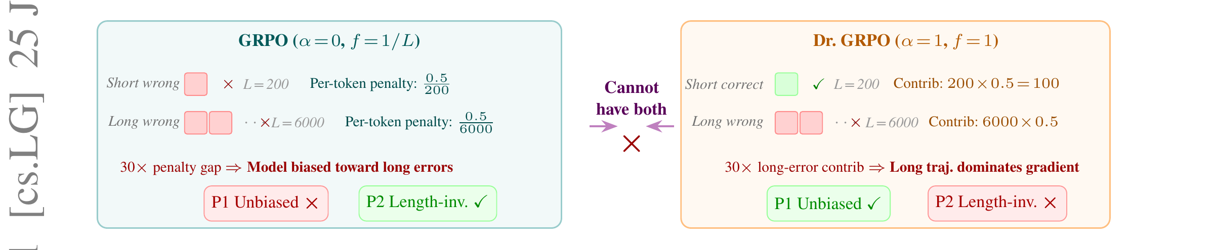
Read the left (teal) box first: under GRPO, a 200-token wrong response and a 6,000-token wrong response get per-token penalties of $0.5/200$ and $0.5/6000$ respectively — a $30\times$ gap in per-token gradient pressure, which is exactly the mechanism that pushes the policy to prefer generating long wrong answers over short wrong ones (since the per-token cost of being wrong is diluted by length). The right (orange) box shows Dr. GRPO’s opposite failure: a 200-token correct response contributes $200 \times 0.5=100$ to the gradient while a 6,000-token wrong response contributes $6000\times0.5=3000$ — the wrong-but-long trajectory swamps the correct-but-short one by $30\times$ in raw gradient magnitude, regardless of correctness. Neither box gets both “P1 unbiased” and “P2 length-invariant” checked simultaneously — this is the theorem rendered as arithmetic.

Figure 2 (paper Fig. 2): the Pareto frontier itself.

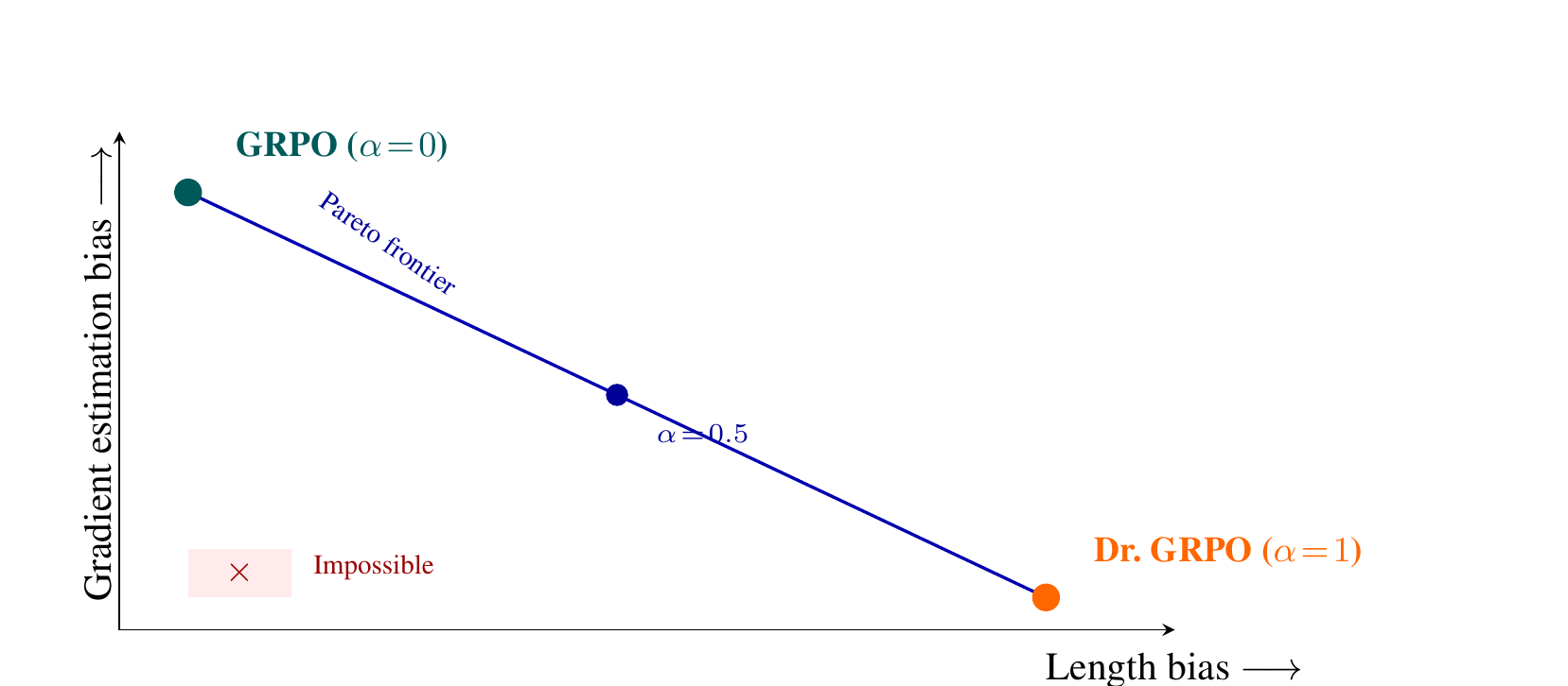
This is the cleanest single visual summary of the whole paper: gradient estimation bias (vertical axis) decreases monotonically as length bias (horizontal axis) increases, moving from GRPO through $\alpha=0.5$ to Dr. GRPO. The shaded box at the origin — zero bias on both axes simultaneously — is the region Theorem 6 proves is unreachable. Every real algorithm using a length-only weight function lives somewhere on or above this frontier curve, never inside the forbidden corner.

Table 1 (paper Table 1): the length-ratio arithmetic, tabulated.

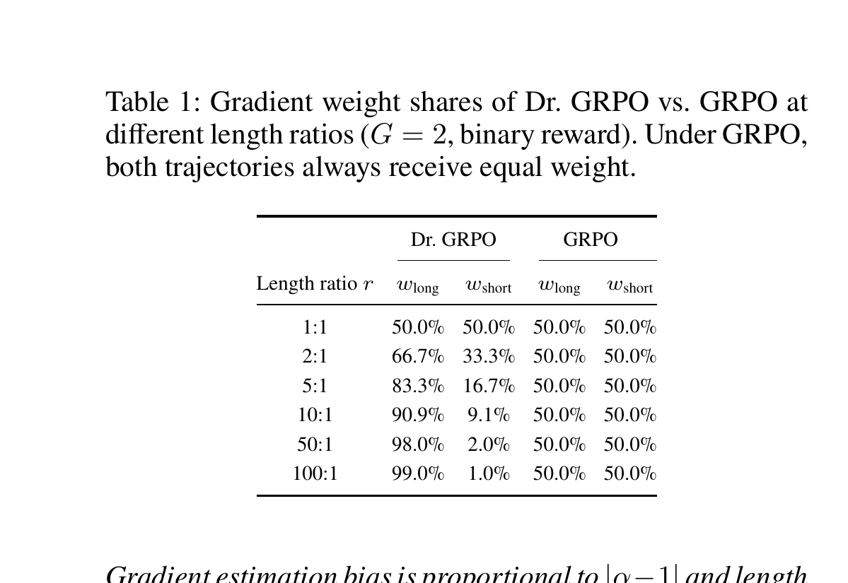
This table is Corollary 9 made concrete: at a length ratio of $r=100{:}1$, Dr. GRPO gives the longer trajectory $99.0\%$ of the total gradient magnitude, versus GRPO’s constant, length-blind $50.0\%/50.0\%$ split. The derivation (Corollary 9’s proof): with $G=2$ and binary reward, exactly one trajectory is correct, giving $\text{mean}(R)=0.5$ and $|\tilde A_1|=|\tilde A_2|=0.5$. Under Dr. GRPO ($f\equiv1$), each trajectory’s gradient contribution magnitude is $f(L_i)\cdot|\tilde A_i|\cdot L_i = 1 \cdot 0.5 \cdot L_i$, so the share is simply $w_i = L_i/(L_1+L_2)$ — for length ratio $r=L_{\max}/L_{\min}$, this is $w_{\text{long}} = r/(1+r)$ (Eq. 35), which is $50\%$ at $r=1$ and $\to 100\%$ as $r \to \infty$. Under GRPO ($f(L)=1/L$), the contribution is $(1/L_i)\cdot 0.5 \cdot L_i = 0.5$ for every $i$ — independent of length, by construction.

Corollary 12, worked out — GRPO’s own bias, quantified. The paper doesn’t let GRPO off the hook either. Corollary 12 states GRPO’s gradient estimator satisfies:

$$\mathbb{E}[\hat{g}_{1/L}] - \nabla_\theta J = \mathbb{E}\left[\frac{1}{G}\sum_i \tilde{A}_i\left(\frac{1}{|o_i|}-1\right)\nabla_\theta\log\pi_\theta(o_i \mid q)\right] \tag{36}$$

Proof, step by step: by direct computation, $\mathbb{E}[\hat g_{1/L}] = \mathbb{E}\left[\frac{1}{G}\sum_i \tilde A_i \frac{1}{|o_i|}\nabla_\theta\log\pi_\theta(o_i\mid q)\right]$, while the true gradient is $\nabla_\theta J = \mathbb{E}\left[\frac{1}{G}\sum_i \tilde A_i \nabla_\theta\log\pi_\theta(o_i \mid q)\right]$ (this is just Eq. 2 specialized to constant per-trajectory advantage). Subtracting the two and using linearity of expectation gives Eq. (36) directly. This bias is non-zero precisely when $|o_i|$ (the length, which is determined by when the policy decides to emit EOS) is statistically dependent on the score function $\nabla_\theta \log \pi_\theta(o_i \mid q)$ — and the paper correctly points out this dependence is essentially always present, because the policy itself controls both the content (which determines the score) and the stopping time (which determines the length). This is a genuinely elegant observation: it’s not that length happens to correlate with the gradient by coincidence in some datasets; it’s structurally true because the same network parameters generate both.

Example 11 — anchoring the theorem in a real training log. Liu et al. (2025) reported DeepSeek-R1-Zero produces correct answers averaging 4,965 tokens and incorrect answers averaging 8,206 tokens — roughly a 1:1.65 ratio. Plugging this into the Dr. GRPO weight-share formula ($w_i = L_i/(L_1+L_2)$ with $G=2$): the incorrect (longer) trajectory captures $8206/(4965+8206) \approx 62.3\%$ of the gradient, a 24.6 percentage-point deviation from the naively-expected 50/50 balance. The paper is careful to note this specific number is a single-pair illustration rather than a full-scale replicated ablation — but it’s a real, already-published pair of numbers, not a synthetic worst case, which makes the theorem’s practical bite concrete rather than purely hypothetical.

Putting it all together — a decision-flow view of the diagnostic algorithm. Section 3.3’s Algorithm 1 and this section’s worked examples compose into a single practical decision procedure a training engineer could actually run against a live job:

flowchart TD
    Start["Observe: response lengths growing<br/>during RLVR training"] --> Q1{"Is length variance<br/>within a group high?"}
    Q1 -->|"No (lengths similar)"| Neg["Tradeoff is negligible —
    either f choice is fine (Section 4.2 'when does
    the tradeoff matter' guidance)"]
    Q1 -->|"Yes (e.g. correct vs.
    incorrect differ 2x+ in length)"| Q2{"Which failure mode
    are you more worried about?"}
    Q2 -->|"Model drifting toward
    verbose wrong answers"| UseGRPO["Lean toward α closer to 0
    (GRPO-like): length-invariant,
    accept some gradient bias"]
    Q2 -->|"Correct-but-short answers
    under-reinforced vs.
    long ones"| UseDrGRPO["Lean toward α closer to 1
    (Dr.GRPO-like): unbiased gradient,
    accept length-driven weight skew"]
    UseGRPO --> Monitor["Monitor Corollary 12's
    bias term + weight-share spread
    (Algorithm 1) over training"]
    UseDrGRPO --> Monitor
    Monitor --> Adjust["Adjust α per curriculum-phase
    guidance (Section 5 'practical guidance') —
    exploratory, not theorem-derived"]

Figure C (self-drawn): a practitioner-facing decision tree synthesizing the paper’s theorem, corollaries, and informal guidance into one flow — note the last step is explicitly heuristic, not part of the proof.

6. Limitations (as stated, and as I’d extend them)

As the authors state them: the impossibility result is specific to the outcome-reward setting, where a single scalar reward is broadcast identically to every token in a trajectory. Under process rewards (Schulman et al., 2018-style step-level rewards), different tokens get different advantage estimates, the advantage is no longer constant within a trajectory, and the clean $|o_i|\cdot\tilde A_i$ factorization this paper’s corollaries depend on breaks down — extending the impossibility analysis to that setting is explicitly flagged as future work. The analysis is also single-step: it says nothing directly about how length bias interacts with multi-step optimization dynamics (PPO-style clipping across many gradient steps, learning-rate schedules, or how the causal chain from “gradient dominance” to “actual behavioral drift toward longer outputs” plays out over hundreds of updates) — this too is explicitly called out as beyond the paper’s scope.

What I’d add: first, the theorem is stated over an idealized policy class satisfying “fixed-length realizability” (Assumption 2) — real neural policies never produce a literally fixed length almost surely, so the theorem’s guarantee is a statement about the achievable estimator family, not a direct proof that any specific real training run is currently mis-weighted by exactly this much; how tightly the bound bites depends on how close a real policy’s conditional length distribution gets to violating the non-triviality condition, and this paper offers no empirical measurement of that gap for a real trained model (Example 11 uses marginal average lengths from a training log, not the conditional distribution $\Gamma_{\pi,\rho}(L;a)$ the theorem actually requires). Second, the “scope” caveat that only length-only weighting is ruled out is doing a lot of quiet work — it means results like DAPO’s or other length-aware clipping/masking schemes that condition on more than raw length aren’t automatically covered by this impossibility, and the paper doesn’t map out which of the many “fixed” GRPO variants in the wild are actually still length-only functions in disguise (many token-level or advantage-clipping schemes effectively still reduce to some $f(L)$ once you trace through the algebra, but the paper doesn’t do this audit for the reader).

7. Critical Analysis

Weaknesses and flaws specific to this paper. The theorem, while genuinely elegant, rests on a somewhat convenient existence assumption (Assumption 2, fixed-length realizability) that is never operationalized or checked against any real policy — the entire quantitative “bite” of the theorem (how big is the tradeoff in practice, for a specific model and dataset) is asserted via a single illustrative pair of numbers (Example 11’s 4,965 vs. 8,206 tokens) rather than measured directly from the theorem’s own object of study, $\Gamma_{\pi,\rho}(L;a)$, on any actual trained checkpoint. A paper whose central claim is “this bias is quantitatively severe in realistic training regimes” would be considerably stronger with at least one small controlled experiment measuring the actual conditional length-advantage distribution during a live RLVR run, rather than relying entirely on a single previously-published marginal statistic pulled from a different paper’s table.

Limitations the authors understate or omit. The paper is candid about scope limitations (outcome-only, single-step) but somewhat understates how much of the practical debate this doesn’t resolve: knowing that “GRPO and Dr. GRPO are two Pareto-optimal points” doesn’t tell a practitioner which point is preferable for their specific training regime, and the “practical guidance” offered (Section 5: use smaller $\alpha$ when length variance is high, larger $\alpha$ early in training) is heuristic, not derived from the theorem itself — it’s post-hoc intuition dressed in the same section as a rigorous proof, and a careful reader should notice the change in epistemic register between Sections 3-4 (proof) and the guidance paragraphs (informed opinion). The paper also doesn’t address the fact that many production RL pipelines (DAPO, GSPO, and others already reviewed on this blog) apply length normalization at the sequence level combined with token-level importance-ratio clipping in ways that may not be cleanly representable as a single scalar $f(L)$ at all — the “unified framework” claims to cover “GRPO and Dr. GRPO,” but its coverage of the broader post-2024 zoo of length-handling tricks is implicit at best.

Concrete, specific improvement suggestions. (1) Add a small empirical section — even a single 7B model, single dataset ablation — measuring the actual realized weight-share spread $w_{\text{long}} - w_{\text{short}}$ during a live training run under both GRPO and Dr. GRPO, to show the theorem’s predicted gap (Table 1’s arithmetic) actually manifests in gradient norms, not just in the idealized $G=2$ toy calculation. (2) Extend the parametric family analysis to derive, rather than heuristically suggest, a length-variance-adaptive $\alpha(t)$ schedule — the paper gestures at “a curriculum approach could be beneficial” in one sentence but doesn’t attempt to formalize what an optimal schedule would look like even under simplifying assumptions. (3) Explicitly classify at least the 3-4 most-cited post-GRPO length-handling variants (Dr. GRPO, DAPO’s length penalty, GSPO’s sequence-level ratio, RLOO) by where they sit on or off this Pareto frontier — right now the paper leaves this as an exercise for the reader, but doing it in the paper itself would make the “unifying framework” claim actually earn its name rather than just unifying the two most famous cases.

8. Reproducibility Notes

This is a pure-math paper with no training runs, so “reproducibility” here means checking the proofs and the arithmetic, both of which are fully checkable by hand:

• Theorem 6’s proof (Section 3, three steps) is self-contained and uses only the score-function identity $\mathbb{E}_\pi[\nabla_\theta\log\pi_\theta(o)]=0$ and linearity of expectation — no external results are needed beyond the REINFORCE identity, which is standard (Sutton & Barto, 2018).
• Corollary 9’s table (Table 1) is directly recomputable: for any length ratio $r$, $w_{\text{long}} = r/(1+r)$ under Dr. GRPO, constant $0.5$ under GRPO — plug in $r \in \{1,2,5,10,50,100\}$ to reproduce every row.
• Example 11’s number ($62.3\%$) is directly recomputable from the publicly reported DeepSeek-R1-Zero average lengths (4,965 correct / 8,206 incorrect): $8206/(4965+8206) = 0.6229\ldots$
• No code, checkpoints, or datasets are released or needed — the entire artifact is the argument itself, which is a genuine strength for a paper making a foundational claim about an entire algorithm family.

8.5 Extension to General Group Size: Corollary 13, Unpacked

The paper doesn’t stop at $G=2$. Corollary 13 generalizes the length-bias arithmetic to arbitrary group size $G$ with binary reward: if $K$ out of $G$ sampled responses are correct, the advantages become $\tilde A_{\text{correct}} = 1 - K/G$ and $\tilde A_{\text{incorrect}} = -K/G$ (this follows directly from Eq. 3: correct responses get reward 1, incorrect get 0, and the group mean is $K/G$). Under Dr. GRPO, the effective weight of trajectory $o_i$ generalizes from the $G=2$ special case to:

$$w_i = \frac{|o_i| \cdot |\tilde{A}_i|}{\sum_{j=1}^{G} |o_j| \cdot |\tilde{A}_j|} \tag{37}$$

Why this matters beyond the $G=2$ toy case: production RLVR runs almost never use $G=2$; DeepSeek-R1-style pipelines commonly sample $G=8, 16,$ or even $64$ responses per prompt to get a reliable group-relative baseline. Eq. (37) shows the length-bias mechanism identified in Corollary 9 doesn’t require exactly two trajectories to bite — it holds for any group size, and the qualitative conclusion is unchanged: longer trajectories always contribute more to the gradient under Dr. GRPO, regardless of their correctness. This is worth dwelling on, because it rules out a natural objection (“maybe the bias is just a small-$G$ artifact that washes out with bigger groups”) — the proof structure (Corollary 9’s derivation, generalized) shows the bias is intrinsic to the $f\equiv 1$ weighting itself, not a finite-sample quirk of small groups.

A subtlety worth flagging: at larger $G$, you’d naively expect the relative impact of any single long outlier trajectory to shrink, since it’s now one of $G$ terms in a sum rather than one of 2. But Eq. (37) shows the weight is a ratio of that trajectory’s $|o_i|\cdot|\tilde A_i|$ against the sum of all $G$ trajectories’ same quantity — so if the length distribution across the group is itself skewed (a few very long incorrect trajectories among many short correct ones, which is exactly the empirically observed pattern in reasoning RL), the outlier’s share doesn’t shrink proportionally to $1/G$; it shrinks only to the extent the other trajectories in the group are themselves long. In the regime where correct answers are uniformly short and incorrect answers are heterogeneously long, a single very-long incorrect outlier can still dominate a group of $G=16$ almost as thoroughly as it dominates a group of $G=2$.

9. Where This Sits in the Broader Efficient-RL-Training Landscape

This paper is best read alongside the broader 2025-2026 wave of “what exactly is GRPO doing wrong” papers this blog has already covered — DAPO’s clip-higher and dynamic sampling, GSPO’s move to sequence-level importance ratios, VAPO’s value-augmented approach, and RLOO’s REINFORCE-style baseline. Nearly every one of those papers makes some choice about how to weight or normalize by length, usually justified with an empirical ablation (“removing X improved Pass@1 by Y points”). What this paper contributes that none of those individually do is a structural argument for why such a choice can never be a clean, bias-free “fix” — it’s always trading one property against another. The practical upshot for anyone reading the next length-handling paper in this space: ask not “did they fix the length bias,” but “which side of this Pareto frontier did they move toward, and is that the right tradeoff for my training regime’s length variance.”

9.5 A Practical Checklist for Reading the Next “We Fixed GRPO’s Length Bias” Paper

Given how many papers in this exact sub-area will keep appearing — length-aware clipping, sequence-vs-token-level importance ratios, adaptive normalization schedules — it’s worth distilling this paper’s machinery into a repeatable checklist you can apply to the next one:

1. Identify the effective weighting function. Does the new method reduce, after algebra, to some $f(L)$ applied uniformly to a trajectory’s gradient contribution? If so, Theorem 6 already tells you it cannot be both P1- and P2-satisfying — the only question is where on the tradeoff curve it sits, not whether it has “solved” the problem.
2. Ask whether the fix is genuinely length-only, or something richer. Per the theorem’s stated scope, methods that condition on token position, local context, or per-token credit assignment (not just the scalar $|o_i|$) are not automatically covered by the impossibility — these are the more promising directions for anything claiming to escape the tradeoff entirely, and deserve a fresh analysis rather than being waved through as “like Dr. GRPO but better.”
3. Check which failure mode the paper’s own ablations are tuned to detect. A paper that only reports overall accuracy improvements, without separately reporting (a) response-length drift over training and (b) some proxy for gradient-estimation bias, is very likely reporting a move along the Pareto frontier dressed up as a strict improvement — ask what got worse.
4. Look for the length-variance context. Per Section 4.2’s “when does the tradeoff matter” discussion, the practical stakes of any $\alpha$ choice scale with how much response lengths vary within a group for the task distribution being trained on. A method validated only on tasks with low length variance (e.g. short-form QA) tells you little about how it will behave on long-chain mathematical or agentic reasoning, where length variance is exactly where this tradeoff bites hardest.
5. Watch for the word “unbiased” used in isolation. As this paper’s whole argument shows, “unbiased” is a true but incomplete description unless paired with an explicit statement about what property was traded away to get it. Any paper using “unbiased” as a synonym for “correct” or “fixed” without acknowledging a corresponding cost is repeating exactly the framing this paper set out to correct.

10. Conclusion

The headline result here is small, provable, and — once you see the proof — obvious in hindsight, which is exactly what makes it valuable: gradient unbiasedness and length invariance cannot coexist under outcome-reward group RL, for any length-only weighting scheme. GRPO and Dr. GRPO are not a broken algorithm and its correct successor; they’re two named points on a continuous, unavoidable tradeoff curve, with everything in between (and arguably things outside the length-only family entirely) representing legitimate, different design choices rather than degrees of “correctness.” If there’s one sentence worth remembering from this paper for your next RL training run: don’t ask which length-normalization scheme is unbiased — ask which bias you’re choosing to accept, and whether it matches the length-variance profile of the task you’re actually training on.