BLADE: Boundary-Expanded and Layer-Adaptive Dynamic Exit for Efficient LLM Reasoning

Review date: 2026-08-03 Author: Zhongzhu Zhou Paper reviewed: BLADE: Boundary-Expanded and Layer-Adaptive Dynamic Exit for Efficient LLM Reasoning Paper authors: Keshu Fu, Keqin Peng, Jun Bai, Shuhan Qin, Chen Li, Junzhu Liang, Yefei Chen, Jiaqi Li, Yuanxin Ouyang (Beihang University, BIGAI, Peking University, East China Normal University) arXiv: 2607.28966 Venue/Status: Preprint (cs.CL), July 2026

1. Why this paper, and what problem is it actually solving

Here is a small, almost embarrassing example the authors use to motivate the whole paper. Ask a reasoning model to solve $3x + 5 = 20$. It correctly derives $x = 5$, states “Therefore, the answer is $x=5$,” restates the conclusion twice more for good measure, and then says “Wait, let me verify the result once more,” re-derives the same answer, and restates it a third time. Nothing was wrong. The model was already done three sentences earlier. It just kept going.

This is the “overthinking” problem that has become one of the most discussed inefficiencies in long chain-of-thought (long-CoT) reasoning models: once a model has produced enough reasoning to support a correct final answer, every additional token it generates is pure waste — extra latency, extra compute cost, and in some documented cases, actively harmful, because continued generation can talk the model out of a correct answer it already reached. The fix people have converged on is called reasoning early exit: train a small, cheap probe that watches the model’s hidden states as it reasons and predicts, at some set of candidate stopping points, whether the reasoning so far is already “sufficient” to answer correctly. If the probe says yes, you stop generation early and force a final answer.

The dominant prior approach (a family the paper calls DEER/LYNX/DTSR-style methods) only looks for stopping points at self-doubt markers — words like “Wait,” “however,” “let me reconsider” — because these words plausibly signal a transition from problem-solving to reflection, i.e., a natural place where a correct answer might already exist. It’s a sensible idea, and it works reasonably well. But look again at the toy example above: the actually correct, checkable, complete answer appears at the very first “Therefore, the answer is $x=5$” sentence — a full three sentences before the first self-doubt marker (“Wait”) ever shows up. Self-doubt-only monitoring, by construction, cannot see this. It has no checkpoint there. The paper’s opening move is to name this precisely: self-doubt checkpoints under-cover the space of sufficient reasoning states. There is a whole class of early-exit opportunities hiding in ordinary sentence boundaries, and the existing literature was blind to them because it only ever looked at self-doubt words.

The obvious fix — just probe at every sentence boundary, not only self-doubt ones — sounds trivial, but it opens up a second, less obvious problem that gives the paper its name. Self-doubt checkpoints are a fairly homogeneous category: they mostly occur at reflection/verification moments, and it turns out a small, fixed subset of hidden layers reliably encodes whether the reasoning up to that point is sufficient. But ordinary sentence boundaries are far more heterogeneous — some are mid-derivation, some complete a key calculation, some restate an already-reached conclusion, some are throat-clearing transitions with no informational content at all. The paper’s core empirical claim is that the layer at which “is this prefix sufficient?” information is most legible depends on what kind of boundary you’re looking at, and a probe design that hard-codes one fixed layer choice (as prior self-doubt-only methods do) becomes measurably worse once you expand to this more diverse checkpoint population. Concatenating all layers avoids that brittleness but is expensive and, as the ablations below show, is not even the best-performing choice — more information is not automatically better information once you’re trying to learn a clean decision boundary from noisy labels.

BLADE (Boundary-Expanded and Layer-Adaptive Dynamic Exit) is the paper’s answer to both problems at once: broaden the checkpoint set to catch the missed opportunities, then learn — per checkpoint population, per model, automatically — a small, informative subset of hidden layers to probe, instead of hand-picking one layer or dumping in all of them. On five math-reasoning benchmarks and two Qwen3 backbones, this combination cuts generated tokens by 24.8% (Qwen3-8B) and 15.8% (Qwen3-4B) relative to full chain-of-thought generation, while keeping accuracy essentially unchanged, and it beats the strongest prior self-doubt-only baseline (LYNX) on the same accuracy-efficiency trade-off metric at every calibration setting tested.

If you work on LLM inference efficiency, test-time compute allocation, or reasoning-model deployment, this paper is a compact case study in a pattern worth internalizing: when a lightweight monitoring signal (self-doubt words) is used as a proxy for a richer underlying phenomenon (prefix sufficiency), it’s worth periodically asking whether the proxy is systematically missing large parts of the phenomenon — and if you expand the proxy’s coverage, whether your downstream model (here, a fixed-layer probe) was implicitly tuned to the old, narrower proxy population and needs to adapt too.

Prerequisites: what you need to know before diving in

If you already know chain-of-thought reasoning, probe-based early exit, and the basics of Transformer hidden-state layers cold, skip to Section 2. Otherwise, here is the minimum vocabulary this paper assumes.

Chain-of-thought (CoT) reasoning and “long-CoT” models. Modern reasoning-tuned LLMs (e.g., the Qwen3 family used in this paper, DeepSeek-R1-style models) are trained or prompted to emit an extended token sequence of intermediate reasoning steps before committing to a final answer. Scaling this “thinking” length at inference time (test-time compute) reliably improves accuracy on hard problems, up to a point — but past that point, additional tokens stop helping and start hurting, a phenomenon the field calls overthinking.

Prefix-sufficiency. For a partial reasoning trace $r_{i,\leq t}$ (everything generated up through some position $t$), we can ask a binary question: if we forced the model to stop right here and just answer, would that answer be correct? If yes, the prefix is “sufficient.” This paper’s entire method is built around learning to predict this binary property cheaply, at various candidate stopping positions, from the model’s own internal hidden states — without ever needing to actually run the “forced completion” at inference time (that is only done during training, to generate labels).

Probe-based early exit. Instead of retraining or modifying the base reasoning model, you attach a small auxiliary classifier (a “probe”) that reads a snapshot of the model’s hidden states at some position and predicts prefix-sufficiency. If the probe is confident enough, generation stops early and a final-answer completion is forced. This is attractive because the probe is cheap to train (order of a few million parameters, versus billions in the base model) and requires zero changes to the reasoning model itself.

Transformer hidden states and layer depth. A Transformer with $L$ layers produces, for every generated token, one hidden-state vector per layer: $h_{i,t,0}, h_{i,t,1}, \ldots, h_{i,t,L-1}$, each in $\mathbb{R}^d$. It is well established in the interpretability literature (going back to work on BERT’s layer-wise behavior) that different kinds of information are more “legible” — i.e., more linearly decodable — at different depths: early layers tend to carry more surface/lexical information, middle-to-late layers more abstract/semantic and task-relevant information, and the right layer for a given probing task is often not obvious in advance and can differ across models and even across different types of probing targets within the same model. This paper’s second contribution (APLS, described below) is precisely about not having to guess this layer choice by hand.

Self-doubt markers vs. sentence boundaries, as checkpoint types. A self-doubt checkpoint is a candidate stopping position right after words like “Wait,” “however,” or “let me reconsider” appear — these are sparse (they show up only when the model second-guesses itself) but fairly reliable signals of a reflection/verification state. A sentence checkpoint is simply the end of any sentence in the reasoning trace (denser, appears constantly, but the underlying reasoning states are far more heterogeneous — some sentences complete the problem, most don’t). A paragraph checkpoint is a coarser boundary used only during training for additional supervision diversity. BLADE’s Multi-Granular Reasoning Checkpoints (MGRC) component, described in Section 3, combines all three.

Accuracy-Efficiency Score (AES). A single scalar metric (defined formally in Section 5) that combines relative token savings and relative accuracy change against a Full-CoT (no early exit) baseline into one number, so that different early-exit methods can be ranked on a single accuracy-efficiency trade-off axis rather than eyeballing two separate numbers.

With this vocabulary in place, the rest of the paper reads cleanly.

2. Architecture overview: what BLADE actually builds

BLADE has two training-time components and one inference-time policy:

1. Multi-Granular Reasoning Checkpoints (MGRC) — construct a diverse pool of candidate stopping positions (sentence + self-doubt + paragraph boundaries) and derive low-noise sufficiency labels for each, via a repeated forced-completion procedure.
2. Adaptive Probe-Layer Selection (APLS) — given those labeled checkpoints, learn which subset of $K$ hidden layers (out of $L$ total) is most informative for predicting sufficiency, rather than hand-picking a layer or using all of them.
3. Boundary-adaptive dynamic exit (inference policy) — at generation time, apply the trained compact probe at sentence and self-doubt checkpoints, using checkpoint-type-aware stopping rules (self-doubt gets to exit immediately on a positive prediction; sentence boundaries need two consecutive positive predictions, because they are noisier).

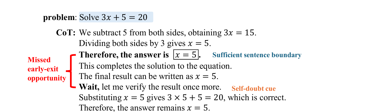
Figure 1 (paper Fig.1): the toy $3x+5=20$ example from Section 1, annotated. The correct, complete answer appears at the first “Therefore” sentence — a sufficient sentence boundary — three full sentences before the first self-doubt cue (“Wait”). Self-doubt-only monitoring has no checkpoint at the earlier position and therefore cannot catch this opportunity.

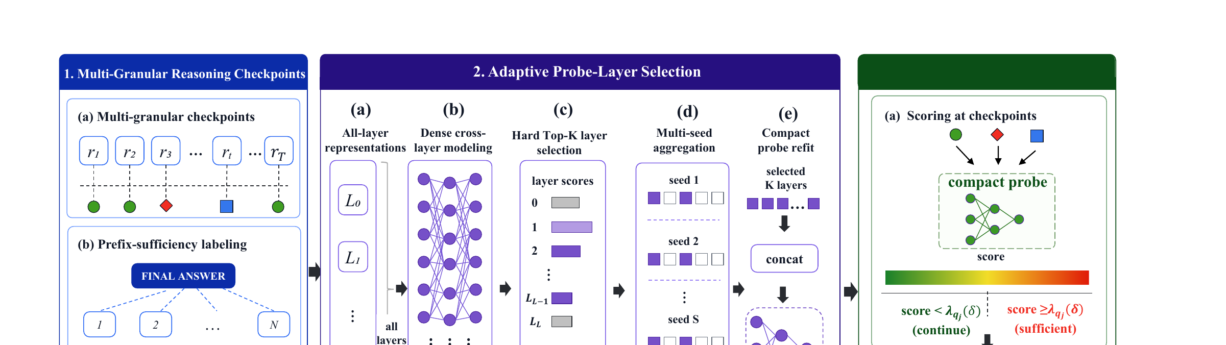
Figure 2 (paper Fig.2): the full BLADE pipeline. Left panel (green header, “1. Multi-Granular Reasoning Checkpoints”): checkpoints of three types are collected along a reasoning trace, and forced-completion sampling turns each into a clean binary label (or discards it as ambiguous). Middle panel (purple header, “2. Adaptive Probe-Layer Selection”): all-layer representations are fed through a dense cross-layer model, which is used to learn a hard Top-K layer mask across multiple random seeds, aggregated by selection frequency, and finally a small compact probe is refit on just the selected $K$ layers. Right panel (dark green header): at inference, the compact probe scores each checkpoint and a calibrated threshold $\lambda_{q_j}(\delta)$ decides continue vs. stop.

Here is the data-flow / pipeline diagram redrawn as a decision flow, which is useful for seeing exactly which parts happen during training (to produce the probe and the layer subset) versus at inference (when a user is actually generating a response):

flowchart TD
    subgraph Training["Training time (offline)"]
        A["Generate reasoning traces on
training problems with base model"] --> B["MGRC: collect sentence + self-doubt
+ paragraph checkpoints along each trace"]
        B --> C["At each checkpoint: force 16 independent
answer completions, keep only unanimous
all-correct / all-wrong labels"]
        C --> D["Train dense cross-layer sufficiency
model on all L layers (frozen after training)"]
        D --> E["APLS: learn hard Top-K layer mask via
straight-through estimator + KD from dense model"]
        E --> F["Repeat layer search across multiple
seeds, aggregate by selection frequency"]
        F --> G["Refit small compact probe on
just the selected K raw hidden layers"]
    end
    subgraph Inference["Inference time (online, per query)"]
        H["Model generates reasoning tokens"] --> I{"Sentence or self-doubt
checkpoint reached?"}
        I -- no --> H
        I -- yes --> J["Compact probe scores prefix
using only the K selected layers"]
        J --> K{"Score >= calibrated
threshold lambda(delta)?"}
        K -- no --> H
        K -- "yes, self-doubt" --> L["Exit immediately,
force final answer"]
        K -- "yes, sentence (1st time)" --> M["Mark tentative,
continue one more checkpoint"]
        M --> N{"Confirmed again
at next sentence checkpoint?"}
        N -- yes --> L
        N -- no --> H
    end
    G -.->|"deployed probe + layer subset"| J

Notice the split: everything expensive (forcing 16 completions per checkpoint, training a dense all-layer model, running multiple random-seed layer searches) happens once, offline, on a training corpus. What actually runs during real inference is just: evaluate a small compact probe on $K$ hidden-state vectors, compare to a threshold, and apply one of two simple stopping rules depending on checkpoint type. This asymmetry — expensive offline search, cheap online deployment — is what makes the resource comparison in Table 4 below (roughly 3x fewer parameters and 6x less peak memory for the deployed probe versus the dense search model) practically meaningful rather than just an ablation footnote.

3. Core theory: prefix-sufficiency and how its labels are derived

3.1 Problem formulation, derived step by step

Given a problem $x_i$, the reasoning model autoregressively generates a token sequence

$$r_i = (r_{i,1}, \ldots, r_{i,T_i}). \tag{1}$$

At any candidate boundary $t$ (a sentence end, a self-doubt cue, or a paragraph end), define the current reasoning prefix as $r_{i,\leq t}$, and collect its layer-wise hidden states across all $L$ Transformer layers:

$$H_{i,t} = (h_{i,t,0}, \ldots, h_{i,t,L-1}), \qquad h_{i,t,\ell} \in \mathbb{R}^d. \tag{2}$$

Now define the central object of the whole paper: a binary prefix-sufficiency variable $Y_{i,t} \in \{0, 1\}$, where $Y_{i,t}=1$ means “if we forced the model to stop generating right here and just produce a final answer, that answer would be correct.” This is not directly observable at inference time (you’d have to actually generate the rest of the reasoning, or force a completion, to know the ground truth) — so the whole point of the probe is to estimate it cheaply from hidden states alone:

$$p_\theta(i, t) = P_\theta(Y_{i,t} = 1 \mid H_{i,t}) = \sigma\big(f_\theta(\Phi(H_{i,t}))\big), \tag{3}$$

where $\Phi$ is a feature extractor that, crucially, only looks at the compact layer subset selected by APLS (Section 4), not the full $H_{i,t}$. Equation (3) is the entire inference-time computation: one forward pass of a small classifier head over a handful of hidden-state vectors, producing a scalar probability.

The hard part is not the probe architecture — it’s small and unremarkable, a projection + prediction head, as we’ll see in Section 4 — the hard part is getting a clean, low-noise training signal for $Y_{i,t}$ at scale. That is what MGRC (checkpoint construction + labeling) solves.

3.2 Multi-granular checkpoint construction

Training candidates are drawn from three complementary checkpoint types, unioned together:

$$\mathcal{C}_i^{\text{train}} = \mathcal{C}_i^{\text{sent}} \cup \mathcal{C}_i^{\text{doubt}} \cup \mathcal{C}_i^{\text{para}}. \tag{4}$$

• $\mathcal{C}_i^{\text{sent}}$ (sentence checkpoints): broad coverage of completed calculations and intermediate conclusions — dense, appears after every sentence, but individually less semantically reliable (most sentences are not sufficient stopping points).
• $\mathcal{C}_i^{\text{doubt}}$ (self-doubt checkpoints): sparse but comparatively reliable reflection/verification markers.
• $\mathcal{C}_i^{\text{para}}$ (paragraph checkpoints): coarse-grained, used only during training to add supervision diversity — notice in Figure 2’s legend that the paragraph checkpoint (blue square) is explicitly marked “train only,” it is never evaluated as a stopping point during actual inference.

The design choice worth dwelling on here: why not just use all possible token positions as checkpoints, for maximum coverage? Two reasons the paper doesn’t say outright but that follow from the setup: (a) most token positions are mid-sentence, structurally very unlikely to be sufficient stopping points, so exhaustively labeling and probing every token would be enormously wasteful for essentially zero marginal early-exit opportunity gained; (b) sentence/self-doubt/paragraph boundaries are natural units where a human (and, empirically, the model’s own generation dynamics) would actually consider “pausing” — they correspond to genuine junctures in the reasoning, which is exactly the property MGRC exploits when it later applies checkpoint-type-aware stopping rules (Section 3.4). Probing at semantically meaningless positions would also make the confirmation-based stopping policy (below) much harder to define sensibly.

3.3 Low-noise prefix-sufficiency supervision, derived

For every candidate boundary $t \in \mathcal{C}_i^{\text{train}}$, the authors do something conceptually simple but expensive: force the model to stop reasoning right there and generate a final answer, and repeat this $N=16$ times independently (sampling introduces variance in what the model outputs when forced to conclude). Let

$$b_{i,t,k} = \mathbb{I}\big[\text{Check}(\hat{a}_{i,t,k}, a_i^\star) = 1\big], \qquad k = 1, \ldots, N, \tag{5}$$

where $\hat{a}_{i,t,k}$ is the answer from the $k$-th forced completion and $a_i^\star$ is ground truth. Equation (5) just says: for each of the 16 forced-completion trials, record 1 if it happened to land on the correct final answer, 0 otherwise.

Now here is the label-construction step, and it is the paper’s single cleverest piece of engineering for reducing label noise:

$$y_{i,t} = \begin{cases} 0, & \sum_{k=1}^{N} b_{i,t,k} = 0, \\ 1, & \sum_{k=1}^{N} b_{i,t,k} = N, \\ \perp, & \text{otherwise.} \end{cases} \tag{6}$$

Walk through what this means: only if all 16 forced completions from this prefix are wrong is the prefix labeled definitively insufficient ($y=0$). Only if all 16 are correct is it labeled definitively sufficient ($y=1$). Any prefix where the 16 trials disagree — some correct, some wrong — is discarded entirely (labeled $\perp$, “unknown,” and excluded from probe training). This is a strict, unanimous-consensus filter, and it deliberately throws away a large amount of data (any genuinely borderline prefix) in exchange for a training signal where the retained labels are about as clean as this kind of stochastic-sampling-based supervision can get. The assumption underlying it: unanimous agreement across 16 independent completions is strong evidence the prefix truly is (or isn’t) sufficient, rather than the model getting lucky/unlucky on a coin-flip; disagreement is treated as a signal of genuine ambiguity that would only inject label noise if force-included.

Design-choice discussion: why unanimity, and what it costs. The obvious alternative is a majority-vote threshold (e.g., label sufficient if $\geq 9/16$ completions are correct), which would retain far more training examples. The paper doesn’t ablate this directly, but the motivation is clear from context: majority-threshold labels would include a substantial fraction of prefixes where the model’s forced answer is essentially a coin flip, and training a probe against such labels risks the probe learning a noisier, less calibrated decision boundary — exactly the problem the whole layer-selection story (Section 4) is trying to avoid downstream. The boundary condition is real, though: on harder benchmarks (AIME-level problems, where even Full-CoT accuracy is only ~50-60%, see Table 1), unanimous-16 agreement is going to be rare, meaning the effective training-label yield on the hardest problems is small, and the probe’s supervision is implicitly skewed toward easier problems where the model’s forced-completion behavior is more deterministic. This is a real limitation the paper doesn’t explicitly flag (see Section 9, Critical Analysis).

3.4 Boundary-adaptive dynamic exit: the inference-time stopping rule

At inference, BLADE evaluates only sentence and self-doubt checkpoints (paragraph checkpoints, recall, are training-only). Because these two checkpoint types differ in density and reliability, applying one uniform stopping rule to both would be a mistake: self-doubt predictions are comparatively trustworthy (sparse, semantically strong signal) so BLADE exits immediately on a confident positive self-doubt prediction. Sentence predictions are noisier and much more frequent, so BLADE requires two consecutive positive predictions at sentence checkpoints before exiting — a simple temporal confirmation filter that catches transient false positives (e.g., a sentence that merely restates an intermediate conclusion without any new synthesis) while still letting persistent sufficiency signals through. Once the stopping condition triggers, the current prefix is retained and immediately followed by a forced final-answer completion; otherwise generation continues to its natural end (or a token budget, in practice).

4. Adaptive Probe-Layer Selection (APLS), unpacked step by step

This is the paper’s second major contribution, and arguably the more novel one — MGRC (broadening checkpoint coverage) is a good idea but a relatively simple one; APLS is a genuinely non-trivial piece of machine learning engineering for turning “which of $L$ layers matter” into an automatic, stable, per-model decision.

4.1 Step 1: dense cross-layer sufficiency modeling

Each layer’s hidden state is independently normalized and projected into a shared feature space:

$$u_{i,t,\ell} = \text{GELU}\big(W_p \, \text{LN}_\ell(h_{i,t,\ell}) + b_p\big). \tag{7}$$

Here $\text{LN}_\ell$ is a per-layer LayerNorm (necessary because raw hidden-state scales can differ substantially across depth), $W_p$/$b_p$ are a shared linear projection, and GELU is the nonlinearity. All $L$ projected features are then concatenated and passed through a dense prediction head:

$$z_{i,t}^T = f_T\big([u_{i,t,0}; \ldots; u_{i,t,L-1}]\big). \tag{8}$$

This dense, all-layer model is trained with class-balanced binary cross-entropy on the unanimous-label set from Equation (6). Once trained, it is frozen — its job from here on is purely to supply a teacher signal for the much harder combinatorial problem of picking a good $K$-layer subset. This is a sensible design choice: solving “which layers matter” and “how do I combine information across layers” simultaneously in one optimization would confound the two questions; freezing the dense model first isolates the second problem (layer selection) as its own well-posed sub-task.

4.2 Step 2: budget-constrained hard Top-K layer selection

Each layer $\ell$ is now assigned one learnable scalar gate logit $\alpha_\ell$, normalized via softmax into a distribution over layers:

$$\pi = \text{softmax}(\alpha). \tag{9}$$

Under a fixed layer budget $K$ (the paper uses $K=4$ throughout), the forward pass constructs a hard binary mask that keeps exactly the top-$K$ layers by gate score:

$$m_\ell^H = \mathbb{I}\big[\ell \in \text{TopK}(\pi, K)\big]. \tag{10}$$

Here is the actual engineering difficulty: Equation (10) is a discrete, non-differentiable operation (you can’t backpropagate through “is this in the top 4”). The fix is a straight-through estimator (Bengio et al. 2013), which the paper writes as:

$$m_\ell = m_\ell^H + \pi_\ell - \text{stopgrad}(\pi_\ell). \tag{11}$$

Working through why Equation (11) does what it’s supposed to: in the forward pass, $\pi_\ell - \text{stopgrad}(\pi_\ell) = 0$ numerically (stopgrad just returns the same value with gradient detached), so $m_\ell = m_\ell^H$ exactly — the discrete hard mask is what’s actually used to compute the model’s output. But in the backward pass, the gradient of $\text{stopgrad}(\pi_\ell)$ with respect to $\alpha$ is defined to be zero, so $\partial m_\ell / \partial \alpha = \partial \pi_\ell / \partial \alpha$ — the gradient flows through the soft, differentiable $\pi_\ell$ as if the hard selection weren’t there. This is the standard straight-through trick: use the discrete decision for the forward computation (so the model actually experiences “only $K$ layers exist”), but use the smooth relaxation’s gradient to update the selection logits, since the true discrete gradient doesn’t exist.

A temporary selection head (used only during this layer-search phase, discarded afterward) evaluates the masked representation:

$$z_{i,t}^M = f_M\big([m_0 u_{i,t,0}; \ldots; m_{L-1} u_{i,t,L-1}]\big). \tag{12}$$

The gate logits and this temporary head are jointly trained using two supervision signals at once: (a) the same class-balanced sufficiency labels used for the dense model, and (b) knowledge distillation from the frozen dense model’s output logits ($z_i^T$ from Equation 8) — i.e., the compact-layer model is trained to both get the label right and to match what the full-information dense model would have predicted. This distillation term is doing real work: it lets the compact model borrow calibration/confidence information from the richer dense model rather than having to relearn everything purely from the (noisier, filtered) hard labels.

4.3 Step 3: stability-aware multi-seed aggregation

Here’s a subtlety the paper is refreshingly honest about: because Transformer layers are residual and heavily redundant (nearby layers carry overlapping information), running the Top-K selection procedure above from different random initializations (“seeds”) does not reliably converge to the same $K$ layers each time. Rather than treating this as a bug to be fixed, BLADE treats it as an expected property and aggregates over it. Run the selection procedure $R$ independent times, and for each layer compute its selection frequency:

$$f_\ell = \frac{1}{R} \sum_{r=1}^{R} \mathbb{I}\big[\ell \in S^{(r)}\big], \tag{13}$$

where $S^{(r)}$ is the Top-K subset found in run $r$. The final adaptive layer subset keeps the $K$ most frequently selected layers across all runs:

$$S^\star = \text{TopK}_\ell(f_\ell, K), \tag{14}$$

with mean gate rank used only to break ties between equally-frequent layers. After fixing $S^\star$, the dense model, the gate logits, and the temporary selection head are all discarded, and a fresh, compact probe is trained from scratch directly on the raw (unprojected) concatenated hidden states of just the $K$ selected layers. This final refit step matters: the earlier stages (dense model, gates, KD) exist purely to identify a good layer subset; once identified, there’s no reason to keep carrying around the machinery used to find it, and training a clean, small probe directly on the raw selected-layer features avoids inheriting any artifacts of the search procedure itself.

4.4 APLS as pseudocode

Algorithm 1: Adaptive Probe-Layer Selection (APLS)

Input: labeled checkpoints {(H_i,t, y_i,t)}, layer budget K, num. seeds R
Output: compact probe P, selected layer subset S*

 1: Train dense cross-layer model f_T on all L layers (Eq. 7-8), class-balanced BCE
 2: Freeze f_T
 3: for r = 1 to R do
 4:     Initialize gate logits alpha^(r) randomly (new seed)
 5:     for each training step do
 6:         pi <- softmax(alpha^(r))                      // Eq. 9
 7:         m^H <- TopK-indicator(pi, K)                   // Eq. 10 (hard mask)
 8:         m <- m^H + pi - stopgrad(pi)                   // Eq. 11 (straight-through)
 9:         z^M <- f_M([m_0 * u_0; ...; m_{L-1} * u_{L-1}]) // Eq. 12 (masked forward pass)
10:         loss <- BCE(z^M, y) + KD_loss(z^M, f_T(all layers))
11:         update alpha^(r), f_M via backprop through Eq. 11's straight-through gradient
12:     end for
13:     S^(r) <- indices of top-K entries of final pi        // this run's selected subset
14: end for
15: for each layer l = 0 to L-1 do
16:     f_l <- (1/R) * sum_r [l in S^(r)]                    // Eq. 13, selection frequency
17: end for
18: S* <- top-K layers by f_l, breaking ties by mean gate rank  // Eq. 14
19: Discard f_T, all alpha^(r), f_M
20: Train fresh compact probe P directly on raw hidden states of layers in S*
21: return P, S*

A hand-worked toy trace of what steps 3-14 accomplish: suppose $L=36$ (a Qwen3-8B-scale model) and $K=4$. In one seed’s run, gate training might converge to $S^{(1)} = \{14, 19, 31, 35\}$; a different seed might land on $S^{(2)} = \{15, 20, 31, 34\}$ — overlapping but not identical, exactly the redundancy phenomenon the paper measures in Figure 5. After $R=10$ such runs, layer 19 (say) was selected in 5 of them, layers 15/31/35 in 3 each, and dozens of other layers in 1-2 runs each; the frequency-aggregation step (13)-(14) then keeps the handful of layers that kept showing up across independent random searches, on the theory that a layer that’s selected by chance in only one run is more likely an artifact of that particular initialization than a genuinely informative signal.

5. Design choices, discussed one at a time

Why checkpoint-type-aware stopping (immediate vs. two-consecutive) rather than one uniform rule? Discussed above (Section 3.4); the alternative — applying the same immediate-exit rule to both self-doubt and sentence checkpoints — is directly tested in Figure 4(b) below (the “Single” curve), and it underperforms the asymmetric policy specifically in the high-accuracy region of the frontier. The boundary condition: this design assumes sentence checkpoints really are noisier on average than self-doubt checkpoints; if a different reasoning-model family produced self-doubt cues that were actually less reliable than sentence boundaries (unlikely but not impossible for a differently-trained model), the asymmetry should in principle flip.

Why reuse the base model’s own hidden states rather than train a separate verifier model? The obvious alternative — train an independent, possibly larger verifier network to judge answer sufficiency from the generated text — would decouple probe capacity from the base model’s own representations, potentially allowing richer judgments. But it would also reintroduce exactly the cost problem early-exit is trying to solve: running a second large model at every checkpoint defeats the purpose of a lightweight probe. Reusing the base model’s already-computed hidden states is essentially free (they exist regardless, as a side effect of the forward pass that’s already happening), which is why the probe here is small (as Table 4 shows: 4.24M parameters for the deployed APLS probe, versus 11.83M for the dense search-time model, both negligible next to an 8B or 4B parameter base model).

Why 16 forced completions, specifically, for label construction, and why unanimity rather than majority vote? Covered in Section 3.3. The boundary condition worth restating here: this is a hyperparameter that trades label quantity for label quality, and the paper doesn’t report an ablation sweeping $N$ or the unanimity threshold — so we don’t know, e.g., whether $N=8$ with unanimity would have been nearly as good at half the label-generation compute cost, or whether a 15-out-of-16 threshold would have retained meaningfully more (still fairly clean) training examples.

Why freeze the dense cross-layer model before searching for a compact layer subset, instead of training everything jointly end-to-end? As discussed in 4.1, this decomposes a hard joint optimization (which layers + how to combine them) into two more tractable sequential ones. The obvious alternative — one joint objective that simultaneously learns gate logits and a lightweight combination head from scratch, without a frozen dense teacher — would remove the distillation signal that seems to meaningfully stabilize compact-probe training (per the KD loss term in Algorithm 1, line 10). The paper does not ablate “APLS without KD,” so how much of APLS’s advantage specifically comes from having a frozen teacher to distill from, versus from the Top-K search mechanism itself, is not separately measured.

6. Experimental results, walked through with the paper’s own figures

6.1 Setup, in brief

Five benchmarks spanning easy to very hard: GSM8K-test, MATH-500, AMC 2023, AIME 2024, AIME 2025 (1,919 questions total, split 192 calibration / 1,727 held-out test). Two backbones: Qwen3-8B and Qwen3-4B. Both the dense teacher and the compact probe are trained on a 6,000-question corpus (2,000 each from GSM8K train, the numeric-answer subset of MATH train, and DeepScaleR train), for 100 epochs, with the strict unanimous-16 (“K16 strict-clean”) labeling scheme from Section 3.3. Conformal calibration thresholds $\delta \in \{0.002, 0.003, 0.005, 0.01\}$ are fit on the calibration split and applied unchanged to the test split; smaller $\delta$ means a stricter (more conservative) stopping threshold. The headline metric is Accuracy-Efficiency Score (AES), defined in Equation (15) below.

6.2 The AES metric, derived

$$\text{AES} = \frac{L_b - L}{L_b} + \begin{cases} 3\frac{p - p_b}{p_b}, & p \geq p_b, \\ -5\frac{p_b - p}{p_b}, & p < p_b. \end{cases} \tag{15}$$

Here $p, L$ are the evaluated method’s accuracy and average generated-token count; $p_b, L_b$ are the Full-CoT baseline’s accuracy and token count. Reading Equation (15) term by term: the first term, $(L_b - L)/L_b$, is simply the fraction of tokens saved relative to Full-CoT — positive when the method uses fewer tokens, which any working early-exit method should. The second, piecewise term handles accuracy: if the method’s accuracy $p$ is at or above the baseline $p_b$, it gets rewarded at a $3\times$ multiplier on the relative accuracy gain; if it falls below baseline, it’s penalized at a steeper $5\times$ multiplier on the relative accuracy loss. This asymmetric weighting (reward $3\times$, penalize $5\times$) is a deliberate design choice by the metric’s original authors (Luo et al. 2026, cited by this paper) to make AES conservative about accuracy loss — a method that saves lots of tokens but loses even a little accuracy gets punished more than it would be rewarded for an equivalent-sized accuracy gain. This matters for interpreting Table 1 below: BLADE’s positive AES values are not just “it saves tokens,” they reflect that it saves tokens while accuracy stayed close enough to baseline that the asymmetric penalty term didn’t dominate.

6.3 Main results: accuracy-preserving token savings

Figure 3 (paper Table 1): accuracy (%), average generated tokens, and AES for Full-CoT (“Base”), BLADE with mixed checkpoints (“Ours-Mixed”), BLADE with self-doubt-only checkpoints (“Ours-Doubt”), and the two LYNX baselines, on both Qwen3-8B and Qwen3-4B.

On Qwen3-8B, BLADE (“Ours-Mixed”) achieves the highest average AES (0.213), ahead of LYNX-K16 (0.188) and LYNX-K1 (0.163). It cuts average generated tokens from 7,837 (Full-CoT) to 5,896 — a 24.8% reduction — while accuracy drops only slightly, from 76.8% to 75.2%. Notice something interesting buried in the per-benchmark breakdown: on GSM8K, BLADE’s accuracy is actually higher than Full-CoT’s (93.7% vs. 92.3%), while using less than half the tokens (733 vs. 1705). This is not just noise — it’s consistent with the overthinking story from Section 1: on easy problems, the base model sometimes second-guesses itself into a wrong answer after already reaching the right one, and early exit prevents that from happening. On the hardest benchmark, AIME 2025, the gap essentially vanishes (52.2% vs. 51.9%, both within noise of each other), which is exactly what you’d expect if the harder problems’ reasoning genuinely requires most of the generated tokens — there is less “free” overthinking to trim.

On Qwen3-4B, the same qualitative pattern holds: BLADE reaches AES 0.175 versus LYNX-K16’s 0.109 and LYNX-K1’s 0.127, cutting tokens from 7,618 to 6,414 (15.8%) with accuracy essentially flat (75.6% vs. 75.8%). The smaller relative token savings on the 4B model versus the 8B model (15.8% vs. 24.8%) is worth flagging as an open question the paper doesn’t fully explain: it could reflect the smaller model reasoning more “efficiently” to begin with (less overthinking to trim), or it could reflect the smaller model’s hidden states being less linearly informative for sufficiency prediction, making the probe itself somewhat less accurate at 4B scale. The paper doesn’t disambiguate between these two explanations.

6.4 Robustness across calibration thresholds

Figure 3 in the paper (not separately reproduced here as an image, since it’s a small line plot already summarized by the reported numbers) shows AES at every calibration level $\delta \in \{0.002, 0.003, 0.005, 0.01\}$ for the five-benchmark Qwen3-8B suite: BLADE’s AES advantage over both LYNX variants holds at every single calibration setting tested, and notably the advantage persists under the strictest threshold ($\delta = 0.002$, the most conservative stopping rule) — exactly the regime where a method that only “looks good” at loose, aggressive stopping thresholds would be expected to lose its edge. This robustness-across-$\delta$ check is a reasonable piece of evidence that BLADE’s advantage isn’t an artifact of one favorably-chosen operating point.

6.5 Layer-selection ablation: is automatic layer search actually earning its keep?

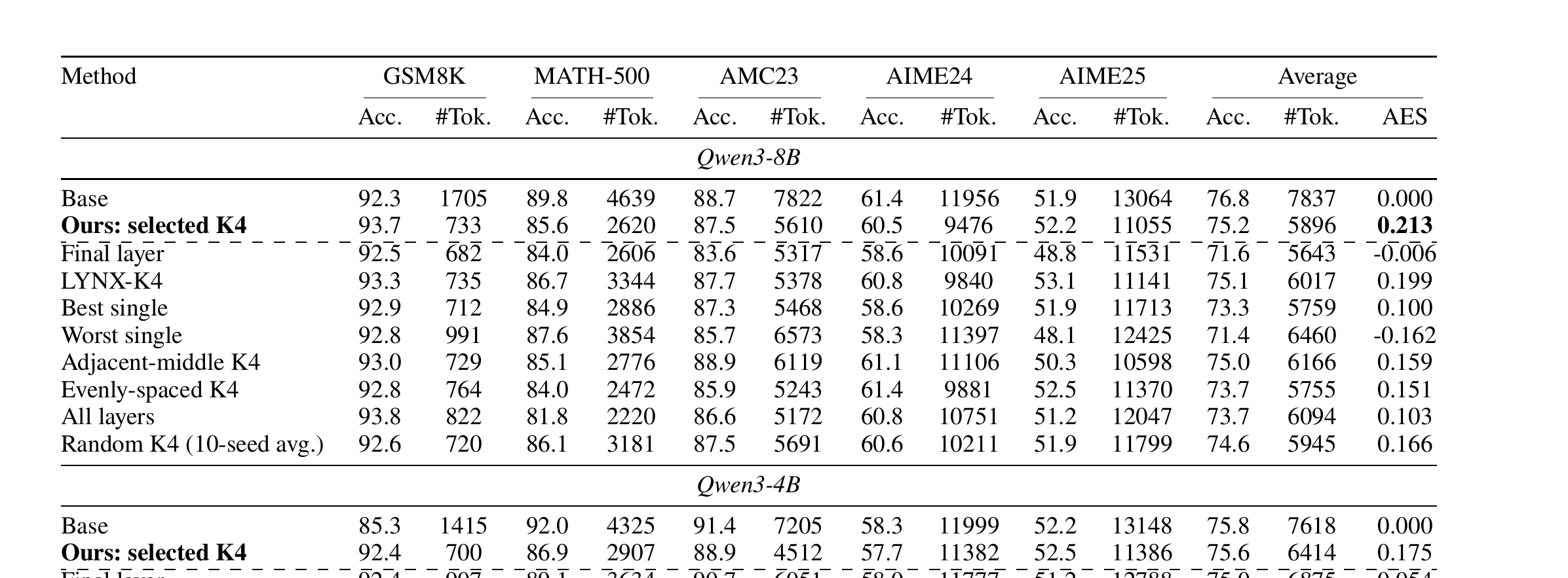
Figure 4 (paper Table 2): comparing BLADE’s automatically-selected $K=4$ layer subset against single-layer probes (best and worst), an all-layer probe, a fixed literature baseline subset (LYNX-K4), and several hand-designed fixed-subset heuristics (final layer only, adjacent-middle four layers, evenly-spaced four layers, random four layers averaged over 10 seeds).

Three comparisons here matter for validating APLS’s core premise:

• Single layer is not enough. The best validation-selected single-layer probe reaches AES 0.100 (Qwen3-8B) — well behind BLADE’s 0.213 — and the worst single-layer probe actually goes negative (-0.162), meaning it’s worse than doing nothing (worse than Full-CoT on the combined accuracy-efficiency trade-off). The gap between best-single (0.100) and worst-single (-0.162) on the same model is itself a striking number: it means the naive strategy of “just pick some layer and probe it” is a genuine gamble, with a huge variance in outcome depending on which layer you happened to guess.
• All layers is not automatically better. Concatenating every layer’s representation yields AES 0.103 (Qwen3-8B) and 0.147 (Qwen3-4B) — both clearly worse than BLADE’s compact 4-layer subset (0.213 / 0.175). This directly supports the paper’s claim that raw information quantity is not the bottleneck; more layers means more redundant and potentially distracting features for the probe to learn to ignore, and a smaller, carefully chosen subset generalizes better.
• Hand-designed fixed subsets are close but not as good, and inconsistent across models. BLADE beats the fixed LYNX-K4 subset on both backbones (0.213 vs. 0.199 on 8B; 0.175 vs. 0.169 on 4B) and beats random 4-layer selection clearly on both (0.166 and 0.151 respectively). Against the “adjacent-middle” and “evenly-spaced” heuristics specifically, though, the picture is more mixed: on Qwen3-8B, BLADE (0.213) clearly beats both (0.159, 0.151); but on Qwen3-4B, adjacent-middle (0.176) and evenly-spaced (0.176) both edge out BLADE (0.175) very slightly — essentially a statistical tie. This is a genuinely useful negative-ish result the paper reports honestly: automatic layer search wins clearly and consistently on the larger model, but on the smaller model, a simple “just spread four layers evenly through the network” heuristic performs about as well, with none of APLS’s training overhead. The paper doesn’t explore why this asymmetry between model scales appears, which would have been a valuable addition (see Critical Analysis).

6.6 Runtime-policy ablations: candidate stream and stopping policy independently

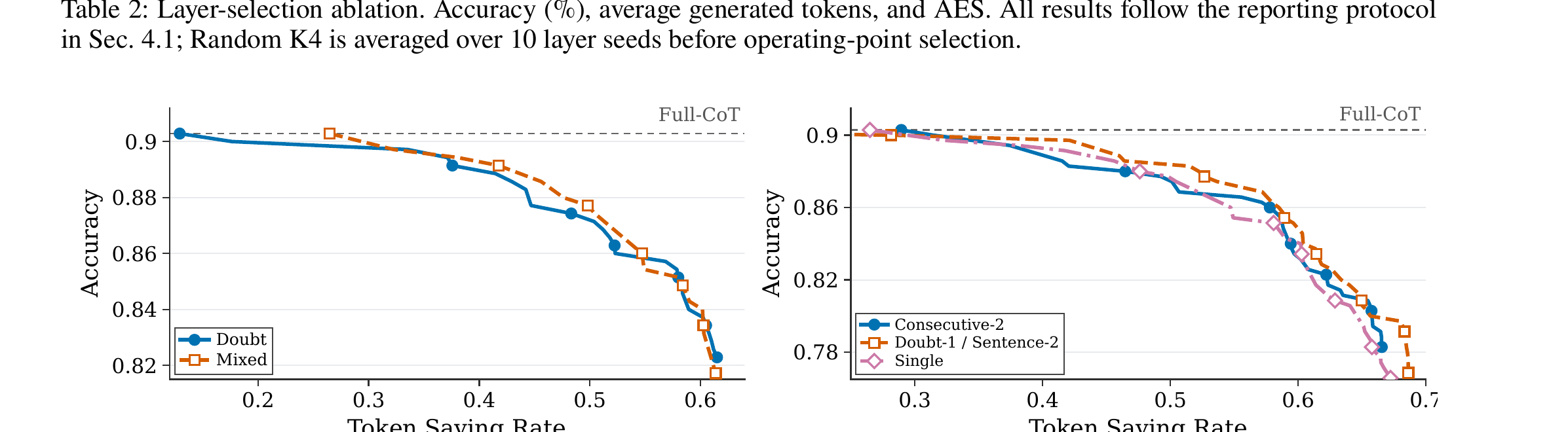
Figure 5 (paper Fig.4): left panel isolates the candidate stream choice (doubt-only vs. mixed sentence+doubt) holding the stopping policy fixed; right panel isolates the stopping policy choice (uniform single-confirmation, asymmetric doubt-immediate/sentence-consecutive-2, or a plain consecutive-2-for-everything rule) holding the candidate stream fixed. Both panels plot the accuracy-vs-token-savings frontier — points further toward the top-right are strictly better (higher accuracy at a given token-saving rate, or equivalently more token savings at a given accuracy).

Left panel: the mixed stream (sentence + self-doubt) traces out a frontier that dominates the doubt-only stream specifically in the high-accuracy region (roughly above 85% accuracy in this plot) — exactly where you’d expect the extra, earlier-arriving sentence-boundary opportunities identified in Section 1 to matter most, since those are the checkpoints that let the model exit before reaching a self-doubt marker at all. Right panel: the asymmetric stopping policy (doubt-immediate, sentence-consecutive-2) traces a frontier that dominates both the naive uniform “consecutive-2-for-everything” rule and a naive “single-confirmation-for-everything” rule, again concentrated in the high-accuracy region. Put together, these two ablations support a specific, falsifiable claim: checkpoint expansion alone is not sufficient — its benefit is contingent on pairing it with a calibrated, checkpoint-type-aware stopping rule. A team that implemented only the MGRC checkpoint-broadening idea, but kept a naive uniform stopping rule, would likely see a noticeably weaker result than what’s reported here.

6.7 Layer-selection stability: are the selected layers meaningful, or just noise that happens to work?

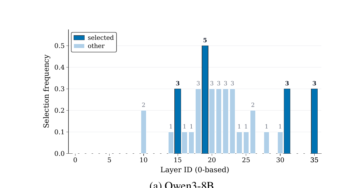
Figure 6 (paper Fig.5): selection frequency (how often each layer index was chosen, out of 10 independent APLS search runs) for Qwen3-8B (top) and Qwen3-4B (bottom). The frequency-aggregated final subsets are $[15, 19, 31, 35]$ for Qwen3-8B and $[19, 21, 22, 27]$ for Qwen3-4B.

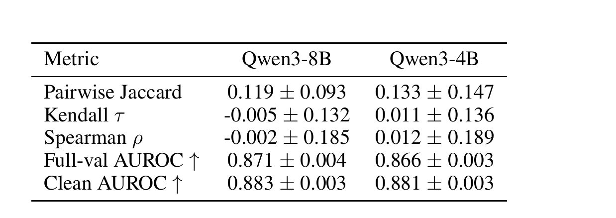
This is the part of the paper I’d flag as the most intellectually honest piece of self-scrutiny: pairwise Jaccard overlap between independently-selected layer subsets is only $0.119 \pm 0.093$ (Qwen3-8B) — meaning two random search runs typically share barely more than one layer out of four — and rank correlations (Kendall $\tau$, Spearman $\rho$) between runs’ full gate-score rankings are essentially zero ($-0.005 \pm 0.132$ and $-0.002 \pm 0.185$ respectively). In plain terms: if you ran APLS’s layer search twice with different random seeds, you would very likely get two noticeably different four-layer subsets, and the overall ranking of all 36 layers by importance would show no meaningful agreement between the two runs either. And yet — this is the striking part — the downstream prediction quality (AUROC) of the resulting compact probes is nearly identical across runs: $0.871 \pm 0.004$ (“Full-val AUROC”) and $0.883 \pm 0.003$ (“Clean AUROC”) for Qwen3-8B, with tiny standard deviations. The paper’s own interpretation (Section 4.5): prefix-sufficiency information is likely redundantly distributed across model depth, because residual-stream Transformer layers progressively update and partially preserve earlier-layer information, so many different four-layer combinations can carry comparably useful evidence for the same underlying decision. The takeaway they draw, which I think is the right one: APLS should be understood as identifying an effective compact representation, not the unique set of mechanistically critical layers — a meaningfully different (and more modest) claim than “we found the layers where sufficiency information lives.”

6.8 Efficiency and resource analysis: does the compact probe actually save resources in practice?

Table 4 (embedded in the same crop above) compares the frozen, discarded dense cross-layer search model against the final deployed APLS compact probe, both evaluated under the same training protocol on Qwen3-8B: parameters drop from 11.83M to 4.24M (roughly a 64% reduction), peak allocated memory drops from 1348.8 MiB to 209.0 MiB (roughly 85% less), and per-epoch training time drops from about 39.87 seconds to 3.97 seconds (roughly a 90% reduction, i.e., an order of magnitude). These are real, concrete infrastructure savings, and they matter because they mean the deployed artifact — the thing that actually runs at inference time, on every checkpoint, for every user query — is cheap, even though the search process used to find it (the dense model plus the 10-seed APLS search) is comparatively expensive. This asymmetry is exactly analogous to how neural architecture search works: expensive one-time offline search, cheap repeatedly-deployed result.

7. Limitations, as the paper (partially) states them and as I read the evidence

The paper’s own conclusion section is quite brief and doesn’t dwell heavily on limitations, so most of what follows is my own reading of what the reported numbers imply, cross-referenced against what’s explicitly acknowledged in Section 4.5 (the layer-selection stability discussion) and the setup details in Section 4.1.

• Domain scope: math reasoning only. All five benchmarks — GSM8K, MATH-500, AMC 2023, AIME 2024, AIME 2025 — are mathematical reasoning tasks with clean, checkable final answers (a number, or a small closed-form expression). This is exactly the domain where the forced-completion labeling scheme (Section 3.3) works cleanly, because “Check($\hat{a}$, $a^\star$)” is unambiguous. It is not obvious the same pipeline transfers cleanly to domains with fuzzier correctness criteria — open-ended code generation, multi-step agentic tool use, or long-form writing — where “forced completion, check correctness” either doesn’t have a crisp binary check, or where forcing early termination changes the nature of the task (e.g., a partially-written function forced to “just answer” doesn’t cleanly map to this framework the way a partially-solved equation does).
• Two backbones, one model family. Both evaluated models are Qwen3 variants (8B and 4B). This is a reasonably standard scope for a paper of this type, but it does mean the observed cross-scale pattern (Section 6.3’s 24.8% vs. 15.8% token savings) is a two-point data series within one family, not a broad scaling-law-style claim across architectures or training regimes (e.g., DeepSeek-R1-distilled models, or non-Qwen bases) that reason rather differently.
• Label yield on hard problems is implicitly reduced by the unanimity filter. As discussed in Section 3.3, the strict unanimous-16 labeling scheme almost certainly discards more of the hardest-benchmark examples (where the model’s forced-completion behavior is closer to a coin flip) than it discards from easier benchmarks. The paper reports the final trained probe’s performance per-benchmark, but does not report the retained-label yield rate broken down by benchmark difficulty, so it’s not possible from the paper alone to judge how much AIME-level performance is being driven by a probe that saw comparatively little clean AIME-difficulty training signal.
• Calibration is done once per model, on a fixed calibration split, not adaptively per problem difficulty. The four $\delta$ values are the same regardless of whether the query is a GSM8K arithmetic problem or an AIME olympiad problem; the reported “best-AES operating point” tables (Table 1, Table 2) select the best $\delta$ per benchmark, which is a fair way to report upper-bound comparisons in a paper, but does not by itself tell a practitioner how to pick a single deployed $\delta$ that will behave well across a mixed, unknown-difficulty production query stream.

8. Critical analysis

Weaknesses and flaws specific to this paper. First, the AES metric’s asymmetric reward/penalty weighting (3x reward, 5x penalty; Equation 15) is imported wholesale from a separate prior paper (Luo et al. 2026) without any sensitivity analysis of how the headline rankings would change under different weighting choices. Since BLADE’s central claim rests almost entirely on AES comparisons, and AES bakes in a specific, somewhat arbitrary trade-off ratio between token savings and accuracy changes, a reader can’t tell from this paper alone how robust the “BLADE beats LYNX” ranking is to, say, a 2x/2x or 4x/6x weighting instead of 3x/5x. Second, the near-tie against “adjacent-middle” and “evenly-spaced” fixed-layer heuristics on Qwen3-4B (Section 6.5) is reported but not explained or investigated further — it’s exactly the kind of anomaly that, per good scientific practice, deserves a follow-up experiment (e.g., does it hold at other values of $K$? does it hold on other benchmarks individually rather than just the macro-average?) rather than being left as an unremarked footnote in a results table. Third, statistical rigor is thin throughout: Table 1 and Table 2’s headline numbers are reported as single point estimates (except for the explicitly-labeled 10-seed random-layer average and the Section 4.5 stability analysis), with no confidence intervals or significance tests on the core AES comparisons between BLADE and LYNX-K16/LYNX-K1. Given that some of the reported gaps are fairly small in absolute terms (e.g., 0.213 vs. 0.199 for BLADE vs. LYNX-K4 on Qwen3-8B, Section 6.5), it would strengthen the paper considerably to know whether these differences are reliably above noise across, say, multiple training seeds of the compact probe itself (not just multiple APLS layer-search seeds, which is a related but distinct source of variance already measured).

Limitations the authors understate or omit. The paper is candid about layer-selection instability (Section 4.5) but does not extend the same scrutiny to probe-training stability more broadly — how much does the final compact probe’s downstream accuracy/token-savings trade-off vary if you retrain it from a different random initialization on the same selected layer subset $S^\star$? This is a different question from the layer-selection-frequency analysis already reported, and it’s the more directly practically relevant one for anyone deploying a single trained BLADE probe in production (they’ll train it once, not average over multiple runs). Separately, the LYNX baselines are re-implemented by this paper’s authors rather than run using the original LYNX authors’ released code/checkpoints (the paper cites Akgül et al. 2025 as the source but describes LYNX-K1/K16 as configurations built for this paper’s comparison); re-implementations of baselines can inadvertently be tuned less carefully than the method being proposed, and the paper doesn’t discuss what steps, if any, were taken to guard against this common source of baseline-disadvantage bias in early-exit / efficient-inference papers specifically.

Concrete, specific improvement suggestions. (1) Report a sensitivity analysis of the AES weighting coefficients (the 3 and 5 in Equation 15), or at minimum report raw accuracy and token-count numbers prominently enough that a reader can recompute rankings under an alternative weighting without needing the underlying data. (2) Run a small additional ablation specifically isolating why adjacent-middle/evenly-spaced heuristics nearly match APLS on Qwen3-4B but not Qwen3-8B — e.g., sweep $K \in \{2, 4, 8\}$ on both models and see if the gap re-opens at a different budget, which would help distinguish “APLS’s advantage is scale-dependent” from ”$K=4$ happens to be a lucky spot for fixed heuristics on this particular model.” (3) Report the retained-label yield rate (fraction of candidate checkpoints that pass the unanimous-16 filter) broken down per benchmark, so readers can judge how much AIME-level supervision the probe actually received versus GSM8K-level supervision. (4) Add confidence intervals (e.g., via probe-retraining across 3-5 seeds on the fixed selected-layer subset) to the main Table 1 / Table 2 AES numbers, distinguishing probe-training variance from the already-reported layer-selection variance. (5) Test on at least one non-math reasoning domain with a fuzzier correctness check (e.g., a code-generation benchmark with unit tests as the “Check” function) to establish whether MGRC’s checkpoint types and the unanimity-filter labeling scheme generalize outside clean, single-number-answer math.

9. Reproducibility notes

The paper reports enough detail to attempt a faithful re-implementation, though several pieces require care:

• Training corpus composition is fully specified: 6,000 questions, 2,000 each from GSM8K train, the numeric-answer subset of MATH train, and DeepScaleR train, split at the question level (important — this avoids checkpoint-level leakage between train and validation within the same problem).
• Label generation is the expensive part to reproduce: $N=16$ forced completions per candidate checkpoint, across every sentence/self-doubt/paragraph boundary in every training trace, means the label-generation phase alone requires a very large number of extra forward-generation calls relative to a single pass over the training corpus — this cost is not explicitly quantified in the paper (no wall-clock or GPU-hour figure is given for label generation specifically, only Table 4’s per-epoch probe training time).
• APLS hyperparameters given: layer budget $K=4$ throughout the main experiments, $R=10$ independent seeds for the multi-seed aggregation (matching the Figure 5 histograms), 100 training epochs for both dense and compact probes.
• Calibration protocol is precisely specified: conformal thresholds fit on a 192-question calibration split at $\delta \in \{0.002, 0.003, 0.005, 0.01\}$, applied unchanged to the 1,727-question held-out test split — this is reproducible as stated, though the exact conformal calibration procedure (which quantile estimator, how ties are broken) is not spelled out in full mathematical detail in the excerpt available.
• Not released as of this writing: the paper does not include a code/checkpoint release link in the version reviewed here, so exact reproduction would require re-implementing MGRC’s checkpoint extraction (sentence/paragraph segmentation logic, self-doubt keyword list) and the full APLS training loop (Algorithm 1 above) from the paper’s description alone.

10. Where this fits in the broader efficient-reasoning landscape

BLADE sits in a fast-moving sub-area of LLM inference efficiency work focused specifically on dynamically shortening reasoning traces without retraining the base model — as opposed to a different family of approaches that train models to reason more concisely from the start (length-penalty RL objectives, distillation onto shorter traces), or approaches that prune/compress the KV cache rather than the number of generated tokens (a topic this same paper-digest series has covered repeatedly, e.g., LOCKS, DynaCalKV, CounterCausalKV, KV-Fold). BLADE is complementary to KV-cache-compression work rather than competing with it: fewer generated tokens directly means a smaller KV cache to begin with, so a system combining early exit with a KV-cache eviction policy would plausibly compound savings from two different axes (fewer tokens generated, and each token’s cache entry cheaper to retain) — though the paper doesn’t test any such combination.

Within the narrower early-exit-for-reasoning sub-area specifically, the field’s central tension (self-doubt-only monitoring is cheap and reliable but under-covers; broader monitoring covers more but needs better-calibrated stopping) is one BLADE addresses directly and, per its own reported numbers, resolves reasonably well for math-reasoning tasks. Whether the same MGRC + APLS recipe generalizes to non-math domains, and whether the near-tie against simple fixed-layer heuristics on the smaller model generalizes to other small models, remain open questions for follow-up work.

11. Conclusion

BLADE makes two contributions that are individually modest but combine into a genuinely useful result: broadening the early-exit checkpoint population beyond sparse self-doubt markers to include ordinary sentence boundaries (catching a real, previously-invisible class of early-exit opportunities), and automating the choice of which hidden layers a lightweight sufficiency probe should look at (avoiding both brittle hand-picked layers and wasteful all-layer concatenation). The reported results — 24.8% and 15.8% token reduction on Qwen3-8B and Qwen3-4B respectively, with accuracy held essentially flat, and the best AES among evaluated methods at every calibration setting tested — are a solid, believable improvement over the self-doubt-only LYNX baselines, and the paper’s own stability analysis (Section 6.7) is a commendably honest piece of self-scrutiny that most papers in this area skip. The main open questions, discussed in Sections 7-8, are about generalization beyond clean math-reasoning benchmarks, the statistical robustness of some of the finer-grained ablation comparisons, and whether the AES metric’s specific weighting choices are driving conclusions that a differently-weighted metric might not fully support. For anyone building or deploying reasoning-model inference systems today, the most directly transferable takeaway is probably not the specific numbers, but the two design principles: check whether your monitoring signal is systematically under-covering the phenomenon you actually care about, and don’t assume a fixed probing layer (or all of them) is the right choice without testing whether an automatically-selected compact subset does better.