FEPLB: Exploiting Copy Engines for Nearly Free MoE Load Balancing in Distributed Training

Review date: 2026-08-02 Author: Zhongzhu Zhou Paper reviewed: FEPLB: Exploiting Copy Engines for Nearly Free MoE Load Balancing in Distributed Training Paper authors: Shuyao Qi, Haoyuan Liu, Shizhen Zhao (Shanghai Jiao Tong University) arXiv: 2604.19654 Venue/Status: Preprint (cs.DC), April 2026

1. Why this paper, and what problem is it actually solving

Here is a number that should bother anyone training a large Mixture-of-Experts (MoE) model: on GLM-5’s MoE layers, with 128 experts and no auxiliary balancing loss, load imbalance wastes 18.6% of GPU time per MoE layer, on average, forever, every single training step. Not once at the start of training. Not only under some pathological data distribution. Persistently, iteration after iteration, because different tokens route to different experts in numbers that fluctuate randomly, and every synchronous training step has to wait for whichever GPU got the unlucky, overloaded slice of tokens that iteration.

The obvious fixes are all bad in one way or another. You could add an auxiliary load-balancing loss to the router, but that constrains what the router is allowed to learn and measurably hurts model quality — which is precisely why frontier MoE models like DeepSeek-V3 have been moving away from auxiliary losses. Or you could accept the imbalance and eat the wasted compute. Or — and this is where prior systems work lives — you could dynamically reshuffle which GPU processes which expert’s tokens, using some form of runtime scheduling. The trouble with that third option, as this paper shows in careful, reproducible detail, is that every previous dynamic-scheduling scheme pays for its flexibility with extra communication, and that extra communication competes for exactly the same hardware (GPU streaming multiprocessors, or SMs, and the inter-node network) that the rest of your parallel training strategy is already using to capacity.

FEPLB’s core insight is refreshingly simple once you see it, and it is the kind of insight that feels obvious in hindsight but apparently nobody had operationalized it for MoE load balancing before: on NVIDIA Hopper GPUs, there is a piece of hardware — the NVLink Copy Engine — that can move data between GPUs on the same node without touching a single SM cycle, and current MoE training frameworks leave it almost entirely idle. If you route your dynamic rebalancing traffic through the Copy Engine instead of through the same collective-communication paths used by Expert Parallelism (EP) and Pipeline Parallelism (PP), you get a genuinely new, hardware-orthogonal parallel dimension for load balancing — one that does not compete with anything else in your training step. That is the whole idea. The rest of the paper is about turning that idea into a system that actually works with unmodified EP semantics, unmodified Grouped GEMM kernels, and a scheduling algorithm cheap enough to run every micro-batch.

If you work on distributed LLM training systems — anything touching MoE routing, EP/PP/TP orchestration, or GPU communication scheduling — this paper is a compact, well-instrumented case study in a broader principle worth internalizing: before building a smarter scheduling algorithm, check whether the bottleneck is actually an algorithm problem or a resource-contention problem. Sometimes the fix is not “schedule better,” it is “find idle hardware and use it.”

Prerequisites: what you need to know before diving in

If you already know Mixture-of-Experts routing, Expert Parallelism, and the NVLink/Copy-Engine distinction cold, skip to Section 2. Otherwise, here is the minimum vocabulary this paper assumes.

Mixture-of-Experts (MoE) layers. Instead of every token passing through one dense feed-forward network (FFN), an MoE layer maintains many smaller FFN “experts” (GLM-5 uses 128) and a lightweight router that, for each token, picks a small subset (top-$k$) of experts to actually run. This lets total parameter count scale into the trillions while the compute per token — and hence the FLOPs cost — stays roughly constant, because only a few experts fire per token. The catch is that the router’s choices are learned and data-dependent, so nobody knows in advance how many tokens will land on any given expert in any given micro-batch.

Expert Parallelism (EP). Since a single GPU cannot hold hundreds of billions of parameters worth of experts, MoE training distributes disjoint subsets of experts across GPUs — e.g., with EP = 8, each of 8 GPUs holds $128/8 = 16$ experts. After the router decides which tokens go where, an all-to-all dispatch communication step physically sends each token’s activations to the GPU hosting its chosen expert, the expert computes, and a combine step sends results back. This dispatch/combine pair is the “standard EP path” that this paper is careful never to modify.

Pipeline Parallelism (PP). The model’s layers are partitioned into sequential stages spread across GPUs (or GPU groups), and micro-batches flow through the pipeline like an assembly line, so that at steady state multiple micro-batches are in flight across different stages simultaneously. PP is orthogonal to EP: EP splits within a layer (which experts live where), PP splits across layers (which layers live where).

Grouped GEMM. When a GPU has to run 16 different experts, each on a different-sized batch of tokens (because routing is uneven), you cannot just call one big matrix multiply — you need a Grouped GEMM kernel that efficiently batches many small, variably-sized matrix multiplications together on the GPU. Crucially for this paper, Grouped GEMM throughput is very sensitive to per-expert batch size: splitting one expert’s token batch into two smaller pieces (say, to move half of them to another GPU) produces two smaller matrix multiplications that run less efficiently in the compute- or memory-bound regime than one larger one. This single hardware fact is why FEPLB’s rebalancing algorithm, as we’ll see, migrates entire experts rather than splitting token batches across devices.

Straggler effect and synchronous training. In standard synchronous data-parallel or expert-parallel training, every device must finish its work for the current step before the optimizer update happens (so all replicas stay numerically consistent). This means the slowest device in each step — the straggler — sets the pace for everyone else. If routing imbalance means one GPU gets 30% more tokens than average this step, every other GPU idles while that one catches up. This paper’s two headline metrics, “token straggler” and “GEMM straggler,” directly measure this excess load on the slowest device relative to the average.

NVLink and the Copy Engine. NVLink is NVIDIA’s high-bandwidth interconnect between GPUs within a node (900 GB/s bidirectional on H100 NVLink 4.0, versus roughly 50 GB/s effective for inter-node RDMA/InfiniBand in this paper’s setup). Normally, when you want to move data between two GPUs — say, via an NCCL collective or a custom kernel — that data movement is orchestrated by kernels running on the GPU’s streaming multiprocessors (SMs), the same compute units that run your matrix multiplies. The Copy Engine is separate, dedicated hardware inside the GPU whose entire job is asynchronous memory copies over PCIe/NVLink; it operates through a distinct hardware data path and does not consume SM cycles or interfere with concurrently-running Grouped GEMM kernels. In other words: you can be running your expert computation on the SMs at full tilt, and simultaneously be shuffling data over NVLink via the Copy Engine, and neither one slows the other down. This paper’s entire systems contribution rests on this one hardware fact.

Resource-level separation, as a design principle. The paper frames its core design principle explicitly: EP and PP both consume RDMA/NVLink bandwidth and GPU SM cycles. If a new “load-balancing parallel dimension” is going to be added without disturbing EP and PP, it must use resources that neither of them touches. FEPLB’s answer: the Copy Engine (for data movement) and idle CPU cycles (for scheduling decisions) — resources current MoE frameworks leave completely unused for this purpose.

With this vocabulary, the rest of the paper reads cleanly.

2. Architecture overview: what FEPLB actually builds

FEPLB introduces exactly one new mechanism, called Two-Phase Dispatch, plus a lightweight CPU-side greedy scheduler that decides, every micro-batch, which experts to rebalance and where. It requires no changes to the EP communication backend (e.g., DeepEP), no changes to the optimizer, and no changes to the model architecture. You keep your existing EP/PP configuration exactly as-is; FEPLB slots in as an additional parallel dimension layered on top.

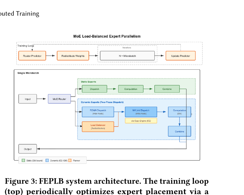
Figure 1 (paper Fig.3): FEPLB system architecture. The training loop (top) periodically re-optimizes expert-to-device placement via a Router Predictor at checkpoint boundaries. Within each micro-batch (bottom), static experts follow the unmodified EP dispatch/compute/combine path (green), while a configurable subset of dynamic experts goes through Two-Phase Dispatch with SM-free NVLink weight redistribution (blue), coordinated by a CPU-side Load Balancer (orange).

flowchart TD
    A["Router assigns tokens to experts\n(this micro-batch's routing decisions)"] --> B["Partition each device's experts:\nstatic (always local) vs. dynamic\n(eligible for redistribution), param dyn"]
    B --> C["Static experts: standard EP dispatch\nto assigned devices (RDMA/NVLink)"]
    B --> D["Dynamic experts: collect tokens from\nentire EP domain into local NVLink domain"]
    C --> E["GPU computes static experts on SMs\n(this is the time window Phase 2 hides in)"]
    D --> F["CPU Load Balancer: greedy\nbusiest-to-least-loaded matching"]
    F --> G["NVLink Copy Engine copies expert\nweights + permuted tokens, SM-free,\n~900 GB/s intra-node"]
    E --> H["GPU computes rebalanced\ndynamic experts on SMs"]
    G --> H
    H --> I["Combine: results returned to\nsource devices via standard EP path"]

The system operates at two distinct timescales. At the macro level, a Router Predictor periodically (at checkpoint boundaries) re-optimizes which experts get assigned to which physical devices, based on accumulated historical routing statistics, spreading out any migration cost over infrequent, cheap events. At the micro level — every single micro-batch — Two-Phase Dispatch does fine-grained, per-step rebalancing to correct whatever imbalance the router happened to produce this step, which is the part of the imbalance problem that a slow, infrequent macro-level re-assignment cannot possibly catch (routing is data-dependent and fluctuates step to step, not just epoch to epoch).

3. Design principle: orthogonal dynamic parallelism, formalized

Before describing the mechanism, it is worth dwelling on the paper’s central design argument, because it is the part most transferable to other systems problems.

The claim: a new parallel dimension for MoE load balancing must be orthogonal to Expert Parallelism (EP) and Pipeline Parallelism (PP) — meaning it must not perturb (1) EP’s inter-node communication pattern or volume, (2) PP’s inter-stage scheduling, and (3) it must consume zero GPU SM cycles, since SMs are the scarcest, most contended resource in the training step.

Why this matters, concretely. The paper walks through exactly why prior dynamic-scheduling systems fail this test:

• Tutel switches between Expert-Parallel and Data-Parallel execution modes at runtime, but doing so requires partitioning expert weights differently across GPUs depending on the mode — which means additional communication to redistribute those weight partitions. It fails orthogonality criterion (1): it perturbs EP’s communication footprint.
• SmartMoE selects among a menu of pre-computed parallel strategies. This is more flexible than a single static strategy, but the menu itself was computed offline under an assumption of known, stable routing statistics — brittle under MoE’s actual data-dependent, per-micro-batch fluctuation.
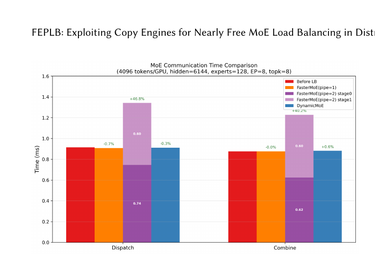
• FasterMoE replicates “hot” (overloaded) experts within the EP domain (a “shadow expert” mechanism) and pipelines the dispatch communication with computation to hide latency. The problem: pipelining requires splitting a single bulk transfer into multiple smaller staged transfers, and modern bulk-transfer communication libraries like DeepEP are optimized for large, single-shot transfers — splitting a transfer into stages on top of DeepEP does not overlap for free, it adds additional communication volume. The paper’s own re-implementation of FasterMoE (Section 3.3, discussed below) measures this directly: pipelined FasterMoE (pipe=2) adds 46.8% extra dispatch time and 40.2% extra combine time relative to the unpipelined baseline. It fails criterion (1) badly.
• Triton Distributed fuses tensor-parallel MoE computation with communication inside custom Triton kernels. This is clever, but the fusion means the SMs themselves are now doing communication work in addition to compute work — the paper measures this costing 1.6–3.3x slower forward-pass time than the EP baseline as more GPUs join the collective (more communication work fused into the same kernel). It fails criterion (3) outright: it consumes SM cycles for communication.

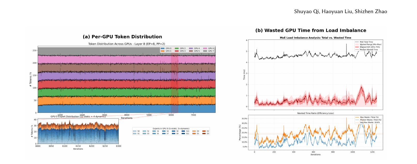
Figure 2 (paper Fig.1): (a) Per-GPU token distribution across 7,000 training iterations for GLM-5’s MoE layer (128 experts, EP=8, no auxiliary loss) shows persistent, random imbalance across all eight GPUs. (b) Wasted GPU time analysis: on average, load imbalance wastes 18.6% of GPU time per MoE layer.

Table 1 (paper Table 1) makes the resource-separation argument in one line:

Dimension	Scope	Communication	Compute
EP	Inter-node	RDMA / NVLink	GPU SMs
PP	Inter-node	RDMA / NVLink	GPU SMs
FEPLB	Intra-node	NVLink Copy Engine	CPU

Every existing parallel dimension in the table shares the same two resource pools: RDMA/NVLink bandwidth and GPU SM cycles. FEPLB is the only row that uses neither — it is intra-node only, its communication rides the Copy Engine (a physically distinct data path from RDMA), and its scheduling compute runs on the CPU, not the SMs. This is why FEPLB can, by construction, coexist with any EP/PP configuration without reconfiguring either: there is no shared resource to contend over. This is the paper’s single most important design-choice discussion, and it is worth internalizing as a general systems heuristic — when adding a new capability to an already resource-saturated system, look for literally unused hardware resources rather than trying to interleave more cleverly on the resources everyone else is already fighting over.

The obvious alternative and where it fails. One could imagine trying to interleave FEPLB’s rebalancing communication within the existing RDMA/NVLink path used by EP, using fine-grained time-slicing or priority scheduling to avoid contention. The paper does not test this directly, but the FasterMoE pipelining results are effectively a natural experiment showing what happens: any scheme sharing the same physical channel and same SM-driven kernels as EP’s bulk transfer inevitably adds overhead, because bulk-transfer libraries like DeepEP are optimized for one large uninterrupted transfer, not staged/interleaved ones. The boundary condition for FEPLB’s own approach: it depends on the existence of a genuinely separate, capable hardware data path (Copy Engine + NVLink) with sufficient bandwidth — this exists on Hopper-class GPUs with 900 GB/s intra-node NVLink, but would not exist, or would be far less useful, on older architectures without a comparably fast, SM-independent copy path.

4. Method details, unpacked: Two-Phase Dispatch

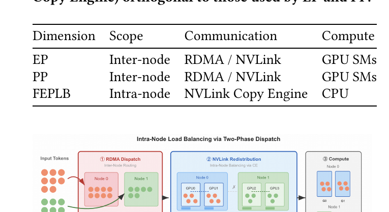
Figure 3 (paper Fig.2): Two-Phase Dispatch. Phase 1 (EP dispatch) routes static-expert tokens inter-node (~50 GB/s) and collects dynamic-expert tokens into the NVLink domain. Phase 2 (NVLink Copy Engine redistribution) copies dynamic-expert tokens and weights intra-node, SM-free, at ~900 GB/s, with no cross-node balancing performed.

4.1 The partition: static vs. dynamic experts

Every device’s local experts are split into two categories, controlled by a single tunable integer $\text{dyn}$:

• Static experts (count $= E_{\text{local}} - \text{dyn}$, where $E_{\text{local}} = 128/\text{EP}$): always processed locally via the unmodified, standard EP dispatch/compute/combine path. These serve a dual purpose beyond just computing model output — their computation time provides the time window during which the CPU scheduler and Copy Engine can do their rebalancing work without blocking the critical path (more on this in Section 4.3).
• Dynamic experts (count $= \text{dyn}$): eligible, this micro-batch, to have their weights (and the tokens routed to them) copied from an overloaded device to an underloaded one via the Copy Engine.

With EP = 8 and 128 total routed experts, each device hosts $128/8 = 16$ experts locally. Setting $\text{dyn} = 4$ makes 4 of those 16 dynamic (rebalance-eligible) and 12 static (always processed locally, no matter the load). This one integer is the paper’s main tunable knob, and Section 6 below examines its sensitivity in detail.

4.2 Phase 1: EP dispatch (unmodified) + dynamic-token collection

Phase 1 runs the standard EP dispatch exactly as any unmodified MoE training pipeline would: the router’s per-token expert assignments are used to send static-expert tokens to their assigned devices via the existing EP backend (e.g., DeepEP), over the normal inter-node RDMA/NVLink path — completely untouched by FEPLB. Simultaneously, tokens destined for dynamic experts are collected from across the entire EP domain into the corresponding local NVLink domain (the local node) and permuted there, in preparation for possible intra-node redistribution. After Phase 1 completes, every device within an NVLink domain knows the exact per-expert token count for its dynamic experts — this is the moment the actual, current-step imbalance becomes visible and actionable.

4.3 Phase 2: NVLink Copy Engine redistribution (the SM-free part)

This is where FEPLB actually differs from doing nothing. The CPU-side load balancer inspects the just-observed dynamic-expert token counts and runs a greedy matching algorithm (formalized as Algorithm 1 below): repeatedly pick the busiest dynamic expert on the most overloaded device, and copy that expert’s weights — plus its already-permuted tokens — to the most underloaded device, subject to a minimum-token threshold $\tau$ that prevents wastefully copying experts with only a handful of tokens (the copy overhead would not be worth it). Crucially, this copy is issued as a Copy Engine transfer on a dedicated CUDA stream, meaning it consumes zero SM cycles and runs fully concurrently with the GPU computing its static experts (Section 4.1’s “dual purpose” time window). Once both the static-expert computation and the weight copy have completed, the GPU computes the dynamic experts using their now-rebalanced load, and a standard Combine step (again over the unmodified EP path) returns results to the tokens’ source devices.

Because each token is still processed by exactly the same expert with exactly the same weights — only the physical device doing that computation has moved — Two-Phase Dispatch preserves exact MoE semantics. This is not an approximation or a routing change; it is a load-transparent relocation of where an already-decided computation happens.

4.4 Algorithm 1, unpacked step by step

The paper’s Algorithm 1 (reproduced and lightly re-annotated below) is the full per-training-step communication rule, including a subtlety the prose description above glosses over: error feedback on the local scaling factors, analogous to error-compensated quantization schemes, to correct for the fact that each dynamic-expert device uses its own local FP-scale rather than a globally synchronized one (this gives better empirical fidelity than synchronizing a global scale, per the paper’s own ablation, at the cost of needing periodic resynchronization).

Algorithm 1: Selective GIFT-style FEPLB Communication
            with Two-Phase Dispatch and Error Feedback
──────────────────────────────────────────────────────────
Require: Fixed selected dynamic-expert set S (size = dyn per device)
Require: Error buffers R^(l) initialized to zero, for l in S
Require: World size N, quantizer Q(.;s), scaling rule Scale(.)

 1: for each training step do
 2:     for each device d do
 3:         for each local expert l with weight-gradient-eligible
             token batch W_g^(l) do
 4:             if l not in S (static expert):
 5:                 // Standard, unmodified EP path
 6:                 dispatch W_g^(l) to assigned device via EP backend
 7:                 compute expert l locally on SMs
 8:                 combine results back via EP backend
 9:             else (l in S, dynamic expert):
10:                 U^(l)      <- collect tokens for l into NVLink domain
11:                 load_d     <- token_count(U^(l))            // observed this step
12:                 // CPU-side greedy scheduling (runs concurrently
                     // with step 6-8's static-expert SM computation)
13:                 if load_d > mean_load + tau:                // overloaded
14:                     target <- argmin_d'( load_d' )           // least-loaded device
15:                     issue Copy-Engine transfer:
                         weights(l) + permuted-tokens(U^(l))  -->  target
                         (SM-free, dedicated CUDA stream, ~900 GB/s NVLink)
16:                 end if
17:                 wait until (static-expert compute AND weight-copy) both done
18:                 compute expert l on its (possibly new) device
19:                 combine results back to source devices via EP path
20:             end if
21:         end for
22:     end for
23:     // Macro-level (infrequent): Router Predictor updates expert-to-device
     //   assignment at checkpoint boundaries using historical routing stats
24: end for

Two implementation details deserve emphasis, because they are exactly the details that make this cheap enough to run every micro-batch rather than periodically:

1. Whole-expert migration, never token splitting. Grouped GEMM throughput is highly sensitive to per-expert batch size (Section “Prerequisites” above); splitting one expert’s tokens across two devices would produce two smaller, less efficient matrix multiplications. So the algorithm always migrates an entire expert’s weights and its full current token batch as one atomic unit — never a fraction of it.
2. Determinism without coordination. Because the greedy algorithm is a deterministic function of the observed per-device token counts (which every device already knows after Phase 1), every device independently derives the same weight-copy plan without any additional coordination round-trip. The paper reports this greedy pass completes in approximately 50 microseconds on a single CPU core — comfortably inside the static-expert computation window it needs to hide behind.

5. The math, expanded: memory overhead and straggler metrics

5.1 Memory overhead derivation

FEPLB must reserve buffer space for copied-in dynamic-expert weights. If $W_{\text{expert}}$ is the per-expert weight size and $\text{max\_num\_dyn}$ is the maximum number of dynamic experts a device might ever need to simultaneously hold copies of, the buffer size is simply:

$$B_{\text{buffer}} = \text{max\_num\_dyn} \times W_{\text{expert}} \tag{1}$$

For GLM-5, each expert occupies 72 MiB. With $\text{max\_num\_dyn} = 8$:

$$B_{\text{buffer}} = 8 \times 72\ \text{MiB} = 576\ \text{MiB} \tag{2}$$

Against an H100’s 80 GB of HBM3 capacity, this is:

$$\frac{576\ \text{MiB}}{80 \times 1024\ \text{MiB}} \approx 0.70\% \tag{3}$$

The design intuition: this buffer is reused across all MoE layers in the model, not allocated once per layer — it is a single scratch region that gets overwritten as different layers’ dynamic experts pass through it during the forward/backward pass. This is why the overhead stays flat (under 1%) regardless of how many MoE layers the model has; if it were allocated per-layer, a deep model (GLM-5’s original 78 layers, versus the 18-layer variant used in these experiments for tractability) would multiply this cost by the layer count and the “nearly free” framing would not hold. This is a design choice worth flagging explicitly: the paper does not dwell on it, but it is load-bearing for the “modest overhead” claim scaling to full-depth production models.

5.2 Token straggler and GEMM straggler, formalized

The paper’s two evaluation metrics are defined precisely as:

$$\text{TokenStraggler} = \max_{d} T_d - \bar{T} \tag{4}$$ $$\text{GEMMStraggler} = \max_{d} G_d - \bar{G} \tag{5}$$

where $T_d$ is the token count assigned to device $d$, $\bar{T}$ is the mean token count across all devices, $G_d$ is the wall-clock Grouped GEMM execution time on device $d$, and $\bar{G}$ is its mean. Both quantities measure the excess load on the single slowest device relative to the group average — precisely the quantity that determines how long every other device idles in synchronous training, since the pipeline (or DP group) cannot proceed past the slowest participant.

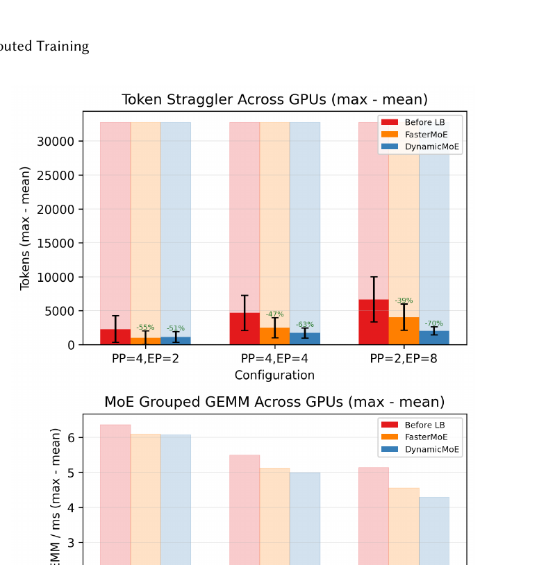
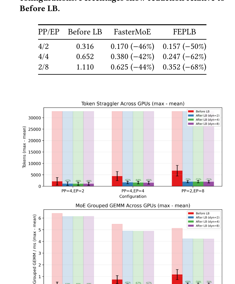
Why report both, rather than just one? Token straggler measures imbalance in the input to the Grouped GEMM (how many tokens land on the busiest device), while GEMM straggler measures the consequence — actual wall-clock compute time wasted. These need not track each other perfectly: Grouped GEMM efficiency is itself a nonlinear function of batch size (very small batches are inefficient per-token; very large batches saturate compute), so a given token-count imbalance can translate into a larger or smaller GEMM-time imbalance depending on where in that efficiency curve the affected experts sit. The paper’s Tables 3 and 4 report both explicitly for exactly this reason — Table 3 (token straggler) shows FEPLB’s advantage growing from 51% to 70% as EP scales from 2 to 8, while Table 4 (GEMM straggler) shows a similar but numerically distinct trend from 50% to 68%, confirming the two metrics are correlated but not identical.

5.3 Deriving the 18.6% wasted-GPU-time headline number

This number (from Figure 1’s motivating measurement, not FEPLB’s own result — it characterizes the baseline problem) comes from:

$$\text{WastedTimeRatio} = \frac{\max_d(\text{LayerTime}_d) - \overline{\text{LayerTime}}}{\max_d(\text{LayerTime}_d)} \tag{6}$$

averaged across 7,000 training iterations of GLM-5’s MoE layer (128 experts, EP = 8, no auxiliary loss). This is the same straggler-vs-average structure as Equations 4–5, but applied to total per-layer wall-clock time rather than token count or GEMM time specifically, and expressed as a ratio of the maximum (so it directly answers “what fraction of this layer’s wall-clock time was wasted waiting for the slowest device”), rather than an absolute gap. The paper’s Figure 1(b) shows this ratio fluctuating noisily between roughly 10% and 25% across iterations, with a reported average of 18.6% — this variance itself is evidence for the paper’s framing that imbalance is a persistent statistical property of routing, not a one-off anomaly correctable by a single static fix.

6. Design choices, discussed: why, what was the alternative, where does it fail

Design choice 1: Copy Engine over SM-based communication. Why it works: the Copy Engine is a physically separate hardware data path from the SMs, so using it for rebalancing genuinely adds zero contention with ongoing compute. The obvious alternative: use a lightweight NCCL point-to-point send/recv or a custom CUDA kernel for the intra-node copy, which would be more flexible (e.g., could fuse a dequantize/requantize step during the copy) but would necessarily consume SM cycles, directly undermining the “orthogonal parallel dimension” claim. Where it fails: the Copy Engine approach is bound by whatever the NVLink topology of the node actually is. On a standard 8-GPU H100 node, all 8 GPUs share one fully-connected NVLink domain, so any-to-any copy within the node is straightforward. On architectures with only partial intra-node NVLink connectivity (older/cheaper node designs), some device pairs might need to route through an intermediate GPU or fall back to a slower PCIe path, which the paper does not address — it is an implicit boundary condition of the whole approach.

Design choice 2: whole-expert migration over token-level splitting. Why it works: preserves Grouped GEMM efficiency, since it never creates a smaller, less efficient sub-batch matrix multiply. The obvious alternative: split an overloaded expert’s tokens proportionally across two or more devices, which would give finer-grained rebalancing control (you could balance load to arbitrary precision rather than in whole-expert chunks). Where it fails, per the paper’s own admission: “current limitations include whole-expert migration without token-level splitting, which limits granularity at low EP.” This shows up concretely in the PP=4, EP=2 result (Section 3.2): with only EP = 2, each device hosts 64 experts, and FEPLB’s backward-pass time (14.4 ms) is very slightly worse than FasterMoE’s (14.0 ms), because at such low EP degree, whole-expert migration cannot subdivide the imbalance finely enough — there simply are not enough independent “chunks” (experts) to redistribute at fine granularity when each device only holds a few dozen experts total relative to the imbalance magnitude.

Design choice 3: greedy busiest-to-least-loaded matching, not an optimal assignment solver. Why it works: it is simple, deterministic (so all devices independently derive the same plan without a coordination round-trip), and fast enough (about 50 μs) to run every micro-batch. The obvious alternative: formulate rebalancing as an optimal transport / min-cost-flow problem and solve it exactly, which could in principle produce a globally better redistribution plan than a greedy pass, especially when multiple devices are simultaneously overloaded and underloaded in complex patterns. Where it fails/why it’s not used: an exact solver would almost certainly take orders of magnitude longer than 50 μs, blowing through the static-expert computation time window it needs to hide inside — the paper implicitly treats “provably optimal” as not worth the latency cost when “good enough, and free” is available on a hardware path that has zero marginal cost anyway.

Design choice 4: dyn as a device-wide static parameter, not adaptive per-step. Why it works: keeps the fast path (for the 12+ static experts on each device, if dyn=4 and EP=8) completely untouched and predictable; a fixed dyn also makes the whole scheme easy to reason about and tune once, offline. The obvious alternative: adapt dyn dynamically based on observed imbalance severity each step (more dynamic experts when imbalance is worse, fewer when it’s mild), potentially squeezing out more of the diminishing-returns tail visible in Figure 6. Where it fails: the paper’s own sensitivity study (Section 7 below) shows diminishing returns beyond dyn=4 are modest (1-3 percentage points from dyn=4 to dyn=8), suggesting the complexity of adaptive tuning would likely not be worth the marginal gain — but this is an empirical claim specific to GLM-5’s routing distribution and profiled workload, and the paper does not test whether a more skewed routing distribution (e.g., from a differently-trained router, or an earlier point in training before routing stabilizes) would shift this tradeoff.

7. Experiments, walked through

7.1 Setup

Hardware: NVIDIA H100 SXM5 GPUs (80 GB HBM3), NVLink 4.0 (900 GB/s bidirectional intra-node), 400 Gbps InfiniBand inter-node. Software: Megatron-LM MoE framework with DeepEP for dispatch, NVIDIA Transformer Engine for mixed precision, multi-stream cuBLAS-based Grouped GEMM, with FEPLB implemented on top (all baselines share identical communication/compute kernels for fair comparison). Model: a reduced-layer GLM-5 variant (18 layers instead of the original 78 — the paper notes that since FEPLB operates independently within each MoE layer, reducing layer count for tractability does not affect the per-layer evaluation), 128 routed experts, top-$k$ routing, no auxiliary balancing loss (i.e., the harder, more realistic imbalance regime). Three PP/EP configurations tested: PP=4,EP=2 (8 GPUs, 64 experts/device); PP=4,EP=4 (16 GPUs, 32 experts/device); PP=2,EP=8 (16 GPUs, 16 experts/device).

Baselines compared: (1) Before LB — plain EP, no rebalancing; (2) FasterMoE, re-implemented by the authors with SM-free NVLink Copy Engine transfers and DeepEP dispatch for fair comparison (both pipe=1 unpipelined and pipe=2 pipelined variants tested); (3) Triton Distributed — TP-parallel fused compute-communication; (4) Tutel — adaptive EP/DP mode switching; (5) FEPLB.

7.2 Per-layer execution time (Figure/Table 2 in the paper)

Figure 2 (paper §3.2, Table 2): Per-MoE-layer forward/backward execution time (ms) across the three PP/EP configurations for Before-LB, FasterMoE, Triton Distributed, Tutel, and FEPLB. Triton Distributed is 1.6-3.3x slower than baseline on the forward pass because its fused communication-computation kernels consume SM cycles that scale worse as more GPUs join the collective. Tutel roughly matches or slightly improves forward time but adds 15-16% backward overhead from weight-partitioning communication. FEPLB consistently matches or beats every baseline: at PP=2,EP=8, forward time drops from 6.9 ms to 6.0 ms (-13%) and backward from 12.5 ms to 10.6 ms (-15%). At PP=4,EP=2 (the low-EP regime discussed in Section 6 above), FEPLB’s forward time ties FasterMoE (7.9 ms) but its backward is marginally worse (14.4 ms vs. 14.0 ms) — the one place in the whole evaluation where FEPLB does not clearly win, attributable directly to the whole-expert-migration granularity limit at low EP.

7.3 Orthogonality verification: does FEPLB actually leave EP communication untouched?

Figure 3 (paper Fig.4): EP communication time (Dispatch and Combine phases) for Before-LB, FasterMoE (pipe=1 and pipe=2), and FEPLB, measured at EP=8. This chart is the paper’s direct empirical test of its central orthogonality claim from Section 3. FasterMoE with pipe=1 shows negligible overhead versus Before-LB, matching FEPLB. But pipe=2 — the pipelined variant meant to hide latency by overlapping dispatch with compute — instead adds 46.8% extra dispatch time and 40.2% extra combine time, exactly the failure mode predicted in Section 3: splitting a bulk DeepEP transfer into pipeline stages adds communication volume rather than hiding it. FEPLB, by contrast, measures below 1% overhead on EP communication in this test, empirically confirming that Phase 2’s Copy-Engine-based redistribution genuinely does not perturb the standard EP dispatch/combine path it runs alongside.

7.4 Load balance quality across configurations

Figure 4 (paper Fig.5): Token straggler (top panel) and GEMM straggler (bottom panel), each as a bar chart across the three PP/EP configurations, comparing Before-LB, FasterMoE, and FEPLB (DynamicMoE in the legend). FEPLB and FasterMoE show opposite scaling trends as EP increases — this is one of the more interesting empirical findings in the paper. At EP=2 (relatively stable routing distribution, since 64 experts per device means any single expert’s token count is averaged over a large “chunk”), FasterMoE’s prediction-based scheduling actually edges out FEPLB slightly on token straggler (55% vs. 51% reduction), though FEPLB already leads on GEMM straggler (50% vs. 46%). But as EP increases to 4 and then 8 (finer-grained expert distribution across more devices, sparser and less predictable per-device routing), FasterMoE’s prediction accuracy visibly degrades — its token straggler reduction drops from 55% to 39% as EP scales up. FEPLB’s purely reactive approach (it observes actual token counts after Phase 1 rather than predicting them ahead of time) improves in the opposite direction, from 51% to 70%. At EP=8, FEPLB achieves 2x lower token straggler (2,021 vs. 4,036 tokens excess) and 1.8x lower GEMM straggler (0.352 ms vs. 0.625 ms) than FasterMoE. The design-level lesson here: prediction-based scheduling degrades as the thing you’re predicting becomes noisier, while a reactive, post-hoc-observation scheme like FEPLB’s is naturally more robust to exactly the kind of unpredictable, data-dependent routing fluctuation that motivates this whole paper.

7.5 Sensitivity to the dynamic-expert count (dyn)

Figure 5 (paper Fig.6): Token straggler as a function of $\text{dyn} \in \{2, 4, 8\}$ across the three PP/EP configurations. Even $\text{dyn}=2$ achieves substantial straggler reduction, because — per the paper’s profiling in Figure 3 of the original paper (the vulnerability-ranking chart used for the closely related GIFT paper’s analogous profiling logic, referenced conceptually here) — imbalance in practice tends to be concentrated in a small number of unusually busy experts rather than spread uniformly across all 16-64 experts on a device. Increasing dyn from 2 to 4 yields a further 1-3 percentage point improvement; from 4 to 8, another 1-3 points — clearly diminishing returns. The paper settles on $\text{dyn}=4$ as “a practical default,” a reasonable choice for GLM-5’s specific profiled workload, though as flagged in Section 6 above, this is an empirical tuning choice rather than a theoretically-derived optimum, and could plausibly shift for models/datasets with more extreme routing skew.

8. Reproducing this yourself: what you’d need

The paper is refreshingly concrete about its exact experimental configuration, which makes partial reproduction plausible: Megatron-LM + DeepEP + NVIDIA Transformer Engine + multi-stream cuBLAS Grouped GEMM, on H100 SXM5 nodes with NVLink 4.0 and 400 Gbps InfiniBand. The reduced 18-layer GLM-5 variant (rather than the full 78-layer model) is explicitly chosen for experimental tractability while preserving per-layer evaluation validity, which is a reasonable and clearly-justified simplification for anyone trying to replicate the core mechanism without needing full production-scale infrastructure. What is not fully specified: the exact GLM-5 hidden dimension and routing hyperparameters used in the reduced variant (the paper’s Figure 4 caption mentions hidden=6144, 4096 tokens/GPU, topk=8, which is helpful but scattered rather than centralized in a reproducibility section), and the precise dataset/routing-statistics profile used to generate Figure 3’s vulnerability ranking is not released. A from-scratch reproduction would need: (1) a Megatron-LM MoE checkpoint with a comparable expert count and no auxiliary loss (to reproduce the “hard” imbalance regime); (2) a custom CUDA-stream-issued Copy Engine transfer path, since standard PyTorch/NCCL abstractions do not expose Copy Engine scheduling directly — this is probably the single largest engineering lift for anyone trying to reimplement this from the paper alone; (3) the greedy scheduling logic (Algorithm 1), which is simple enough to reimplement directly from the pseudocode.

9. Limitations, honestly assessed

The paper’s own stated limitation is narrow and specific: “current limitations include whole-expert migration without token-level splitting, which limits granularity at low EP.” This is honest but incomplete — see Section 10 below for what else is understated.

The evaluation is also limited in scope in ways the paper does not dwell on: a single model family (GLM-5), a single hardware generation (H100/NVLink 4.0), and a reduced 18-layer variant rather than the full 78-layer production model. The paper argues (reasonably) that per-layer evaluation validity is preserved because FEPLB operates independently within each MoE layer, but this argument implicitly assumes the macro-level Router Predictor component (which operates across the whole model at checkpoint boundaries) scales the same way — this is not empirically verified at full depth.

10. Critical analysis

(a) Weaknesses and flaws specific to this paper. First, the evaluation reports averaged metrics (mean straggler reduction across an unspecified evaluation window) with error bars that are visibly large in Figures 4-6 — the confidence intervals on token straggler, especially at PP=2,EP=8, span roughly 3,000-10,000 tokens, which is a substantial fraction of the reported mean improvement itself. The paper does not report statistical significance testing (e.g., a paired test across iterations) for its headline percentage-reduction claims, which would strengthen confidence that FEPLB’s advantage over FasterMoE is not an artifact of a particular evaluation window. Second, the 18.6% “wasted GPU time” headline number in the introduction (Figure 1) is measured without FEPLB — it characterizes the baseline problem, not FEPLB’s solution — but the paper never reports the analogous end-to-end wasted-time-ratio metric with FEPLB applied, only the narrower token/GEMM straggler metrics. A reader is left to infer, rather than see directly, how much of that headline 18.6% FEPLB actually recovers in wall-clock terms; converting a 51-70% straggler reduction into an actual step-time speedup requires knowing what fraction of total step time the MoE layer’s imbalance actually represents, which the paper does not connect back to its own opening statistic.

(b) Limitations the authors understate or omit. The paper frames the Copy-Engine approach as broadly applicable “on the NVIDIA Hopper architecture,” but the benefit is explicitly bound by NVLink topology — the paper itself notes “this scope is limited by the current NVLink topology, not by design,” and gestures at GB200 NVL72’s all-to-all 72-GPU NVLink domain as removing the constraint, but does not test on it. Given that most production MoE training today runs on 8-GPU NVLink domains (the topology tested here), the claim that Phase 2 could eventually “rebalance the entire EP group without cross-node communication” on newer hardware is speculative, not measured. Second, the paper does not discuss what happens when load imbalance itself changes rapidly within a single training run — e.g., early in training when the router has not yet stabilized, routing distributions may be far more skewed (or differently skewed) than the profiled window used to justify $\text{dyn}=4$ and the minimum-token threshold $\tau$; the paper implicitly assumes a roughly stationary imbalance distribution across the training run, which is questionable during the initial “router warm-up” phase. Third, the memory-overhead claim (Section 5.1’s “modest, under 1%”) depends on the buffer-reuse-across-layers implementation detail, which is a design choice the paper does not surface prominently — a naive per-layer allocation (which some MoE frameworks might default to) would multiply this cost by the number of MoE layers, and the paper does not discuss what memory-management API changes are needed in Megatron-LM to guarantee this reuse actually happens correctly across arbitrary layer counts and pipeline stages.

(c) Concrete, specific improvement suggestions. First, report the analogous 18.6%-style wasted-time-ratio metric with FEPLB applied, directly alongside the baseline number from Figure 1, so readers can see the actual wall-clock recovery rather than inferring it from straggler-count reductions alone. Second, run and report an ablation on GB200 NVL72 (or, absent access to that hardware, a controlled simulation) to substantiate the claim that all-to-all NVLink topology would let Phase 2 rebalance across the entire EP group rather than just within an 8-GPU node — as written, this is the paper’s most forward-looking claim and its least empirically supported one. Third, test FEPLB’s sensitivity to a genuinely non-stationary imbalance distribution — e.g., profile and evaluate during the first several thousand steps of training from a randomly initialized router, rather than only on an already-warmed-up model’s routing statistics — to characterize whether the fixed $\text{dyn}$ and $\tau$ hyperparameters chosen here generalize to the early-training regime where imbalance is likely worst and rebalancing arguably matters most. Fourth, provide statistical significance intervals (not just descriptive error bars) for the headline straggler-reduction percentages, ideally with a paired comparison methodology across the same set of training iterations for each baseline, to rule out the possibility that some of the reported gap versus FasterMoE reflects evaluation-window variance rather than a robust systems-level advantage.

11. Conclusion

FEPLB is a clean example of a systems paper whose central contribution is not a new algorithm but a new resource: it notices that the NVLink Copy Engine on Hopper GPUs is sitting almost entirely idle during MoE training, and that if you route dynamic load-rebalancing traffic through it instead of through the same RDMA/SM-based paths used by Expert Parallelism and Pipeline Parallelism, you get a genuinely orthogonal parallel dimension for load balancing — one that, by construction, cannot contend with anything else happening in the training step. The mechanism built on top of this observation (Two-Phase Dispatch, a simple greedy scheduler, whole-expert migration to preserve Grouped GEMM efficiency) is unglamorous but effective: 51-70% token straggler reduction and 50-68% GEMM straggler reduction with under 1% measured EP communication overhead, on GLM-5’s MoE layers without an auxiliary balancing loss. The paper’s most transferable lesson for systems researchers generalizes well beyond MoE: before reaching for a cleverer scheduling algorithm to fix a resource-contention problem, check whether there is simply unused hardware sitting nearby that could solve it for free.