Back from the Future: KV Cache Management by Counter-Causal Surprise

Review date: 2026-08-01 Author: Zhongzhu Zhou Paper reviewed: Back from the Future: Key-Value Cache Management by Counter-Causal Surprise Paper authors: Stephen Gould, Anton van den Hengel arXiv: 2607.27600 Venue/Status: Preprint, July 30, 2026

1. Why this paper, and what problem is it actually solving

Every practical long-context LLM deployment eventually collides with the same wall: the KV cache, not the model weights, is what runs you out of GPU memory. A 16K-token context on a 7B model can already push the cache into multiple gigabytes, and once you are trying to serve batches of concurrent long-context requests, or letting a “thinking” model generate 16K tokens of chain-of-thought before it even answers, the cache dominates memory usage completely. The standard fix is eviction: periodically decide which cached key-value pairs are safe to throw away, and keep only a fixed budget of the most useful ones.

The dominant family of eviction methods — H2O, TOVA, PyramidKV, Ada-KV, and their relatives — all share one core assumption: a token’s attention score tells you how important it is. Tokens that receive a lot of attention during generation are “heavy hitters” and get kept; tokens that are rarely attended to get evicted. This paper’s central contribution is a sharp, well-demonstrated argument that this assumption is subtly and systematically broken, and a replacement scoring rule — counter-causal surprise — that sidesteps the problem entirely without any additional training.

The flaw the paper identifies is what I will call self-reinforcing bias: once a token is retained in the cache, it continues to be available to attend to in future decoding steps, which means it can continue to accumulate attention score, which makes it more likely to be retained at the next eviction round. This creates a rich-get-richer dynamic that has nothing to do with whether the token’s information is still useful. Meanwhile a token that states a single, critical, rarely-repeated fact — a patient’s blood type mentioned once in a 400-page clinical record, a key numeric result stated once in a long derivation — may simply never accumulate enough attention to survive the first eviction round, even though the model may desperately need that exact fact three thousand tokens later.

flowchart TD
    A["Token mentioned once,\nlow initial attention"] --> B{"Eviction round:\nscore below threshold?"}
    B -- "Yes, evicted" --> C["Gone forever --\ncannot recover if needed later"]
    D["Token mentioned repeatedly,\nhigh initial attention"] --> E{"Eviction round:\nscore above threshold?"}
    E -- "Yes, retained" --> F["Still visible next round,\ncan accumulate MORE attention"]
    F --> E
    G["Net effect: early winners\nentrench, early rare facts\nnever get a second chance"]
    F --> G
    C --> G

Figure 0 (self-drawn, Mermaid): The self-reinforcing bias loop in attention-score-based eviction. A token that is retained gets more chances to accumulate attention, which further protects it in future rounds; a token that is evicted early is gone permanently, regardless of whether it later becomes relevant. Counter-causal surprise breaks this loop because a token’s score is recomputed fresh from its future context at every refresh, with no dependence on how much attention it accumulated historically.

Counter-causal surprise flips the entire logic of scoring. Instead of asking “how much attention has this token received,” it asks a much stranger question: can this token be predicted from the tokens that come after it? If yes — if a competent language model, looking only at the future context, could have guessed this token with high confidence — then that token’s information has effectively already been absorbed into the future context, and it is safe to throw away. If no — if the token is a surprise even given everything that follows it — then it must be carrying unique information not recoverable from context alone, and it should be protected.

This is a genuinely different axis of information than attention score, it requires zero training, and (this is the elegant part) it can be computed almost for free by reusing exactly the key/value representations the model has already cached, just processed with a different attention mask.

Prerequisites: what you need to know before diving in

If you are already fluent in causal self-attention, KV caching, and the basic idea of attention-based eviction (H2O/TOVA style), you can skip ahead to Section 2. Otherwise, here is the compressed background.

Causal self-attention and the KV cache, in one paragraph. A transformer’s self-attention layer computes, for each token, a query $q$, key $k$, and value $v$. During autoregressive generation, the causal mask ensures a token at position $i$ can only attend to positions $j \le i$ (the past, including itself), never the future. This is what makes left-to-right generation coherent: token $t{+}1$ is predicted purely from tokens $1{:}t$. Since the keys and values for past tokens never change once computed, they are cached (the “KV cache”) so the model does not have to recompute them at every new decoding step — it only computes $q_t, k_t, v_t$ for the new token and appends $k_t, v_t$ to the cache.

Why the cache grows and why that hurts. The cache holds one key vector and one value vector per token per attention head per layer. For long contexts (tens of thousands of tokens) or long generated outputs (extended chain-of-thought reasoning traces), this becomes the dominant memory cost of serving the model — frequently larger than the weights themselves. Since attention over the whole cache is also a compute and bandwidth cost at every decoding step, a smaller cache is not just about fitting in memory: it can also make each step faster.

Attention-based eviction (H2O, TOVA), in one paragraph. The most influential family of eviction methods scores cached tokens by how much attention they have received. H2O accumulates attention weights over the full generation history and evicts tokens whose running total falls below a threshold, subject to keeping a window of recent tokens. TOVA instead looks only at the most recent token’s attention distribution over the cache at the last layer. Both operate on the intuition that “heavily attended tokens are important tokens.” This paper’s whole argument is that this intuition, while appealing, has a specific failure mode worth naming precisely (see Section 3).

What “counter-causal” means. A standard forward pass uses a causal mask: token $i$ can see tokens $1{:}i$. A counter-causal mask does the opposite: token $i$ can see only tokens $i{+}1{:}t$ — the future, not the past. This paper’s central technical trick is to run a second forward pass over the same cached tokens, but with this reversed mask, in order to ask “how predictable is token $i$ given only what comes after it?” Crucially, this second pass reuses the keys and values already sitting in the cache — it does not require recomputing anything from scratch, and it does not require retraining the model to run “backwards.” It is simply a different attention mask applied to the same underlying representations.

RoPE and absolute positions, briefly. Modern transformers (Qwen2.5, LLaMA 3.1, both used in this paper) use rotary position embeddings (RoPE), which encode relative position information directly into the query/key dot products via a rotation that depends on absolute token position. This matters here because the counter-causal pass reuses cached keys (which already carry the correct RoPE rotation for their original absolute position) and computes fresh queries with the same original position IDs — so the relative offsets in the counter-causal attention computation come out correct, even though the direction of masking has been reversed. This is a subtle but important implementation detail the paper is careful to get right.

With this vocabulary in hand, the mechanism in Section 3 below should read cleanly.

2. Architecture overview: the inference/refresh cycle

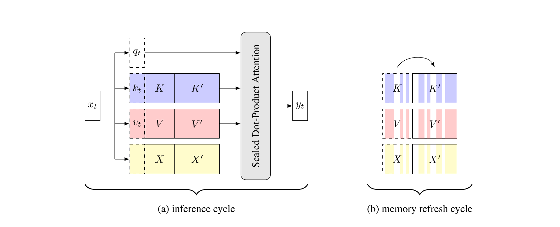
The paper frames its method inside a general two-cycle abstraction that, notably, subsumes sliding-window and heavy-hitter eviction as special cases. Every KV-cache-managed generation system alternates between two operations:

flowchart LR
    A["Inference cycle<br/>(process next token(s),<br/>append k,v to cache K,V)"] --> B{"Cache full /<br/>chunk boundary?"}
    B -- "No" --> A
    B -- "Yes" --> C["Memory refresh cycle<br/>(score all cached tokens,<br/>keep top-J, discard rest)"]
    C --> A

Figure 1 (self-drawn, Mermaid): The inference/refresh cycle that every eviction-based KV-cache manager runs — fill the cache during the inference cycle, then periodically decide what to keep during the memory refresh cycle. Methods differ only in how the refresh cycle scores candidates.

Concretely, the system maintains a small recent-history buffer $K, V$ (holding up to $h$ tokens processed since the last refresh) and a persistent memory $K', V'$ (holding up to $J$ “kept” tokens from before). During the inference cycle, each new token’s key/value are simply appended to $K, V$, and attention runs over the concatenation $K' \oplus K$, $V' \oplus V$ — so nothing is lost from the model’s perspective during normal generation; only the refresh cycle actually discards information. When the recent-history buffer fills up (every $h$ tokens), a refresh cycle fires: it scores every token currently held across $K' \oplus K$ (there are up to $J + h$ of them) and keeps only the $J$ highest-scoring ones, moving them into the new $K', V'$, and clearing $K, V$ for the next chunk.

This chunk-wise design is a practical engineering choice, not incidental to the method: computing a score for every candidate token is itself work, so you do not want to do it after every single token — you batch $h$ tokens’ worth of decisions into one refresh call. The paper is explicit that this generalizes prior methods: sliding window is the degenerate case $J = 0$ (no persistent memory, so $h$ alone defines the whole window), and H2O/TOVA are the case where the refresh-cycle scoring function is “accumulated attention received” rather than counter-causal surprise.

3. The core theoretical claim, unpacked

3.1 The formal object: counter-causal surprise

For a token $x_i$ sitting in the cache at time $t$ (with $i < t$), the paper defines its counter-causal surprise as

$$s_i = 1 - P(x_i \mid x_{i+1:t}) \tag{1}$$

In words: how unlikely is token $i$ given everything that comes after it in the sequence? If $x_i$ is easy to predict from its future context (e.g., a filler word, a grammatically forced token, a redundant restatement of something said more explicitly two sentences later), $P(x_i \mid x_{i+1:t})$ is close to 1 and $s_i$ is close to 0 — low surprise, safe to evict. If $x_i$ is a fact that genuinely cannot be reconstructed from anything after it (a name, a number, a one-off statement), $P(x_i \mid x_{i+1:t})$ is small and $s_i$ is close to 1 — high surprise, must be kept.

This is a clean and intuitively appealing quantity, but it has an immediate practical problem: standard autoregressive LLMs are trained to compute $P(x_i \mid x_{1:i-1})$, not $P(x_i \mid x_{i+1:t})$. They have never seen a training objective that asks them to predict a token from its future; the entire pretraining objective (next-token prediction with a causal mask) runs in exactly the opposite direction. Computing the true reverse-conditional would, in principle, require a separately trained “backwards” language model.

3.2 The approximation: reusing cached K/V with a reversed mask

The paper’s key move is to approximate $P(x_i \mid x_{i+1:t})$ without any additional training, by exploiting a subtlety of how attention actually works. Here is the derivation, spelled out step by step.

Step 1 — what a forward pass with a reversed mask actually computes. Take the same token sequence $x_1, \ldots, x_t$ in its original order, with the original position IDs (so RoPE rotations are unchanged). Instead of a causal (lower-triangular) attention mask, apply a counter-causal (strictly upper-triangular) mask: position $i$ is allowed to attend only to positions $j > i$. Run this through the transformer, and take the output logits at position $i$.

Step 2 — why this approximates the reverse conditional. A standard forward pass with a causal mask at position $i-1$ produces logits that approximate $P(x_i \mid x_{1:i-1})$ because the model has learned, through its entire training process, to use exactly that masking pattern to predict the immediately following token. The counter-causal pass does not have this training-time guarantee — the model was never trained on upper-triangular masks — but the architectural mechanism is identical: at position $i$, the query $q_i$ attends over whatever keys the mask permits it to see, and the output is a function of a weighted combination of the corresponding values, followed by the model’s usual next-token unembedding. Under a counter-causal mask, that weighted combination draws only on tokens $j > i$, so the resulting logit distribution reflects “what does a token that attends only to the future look like,” which is a reasonable, if approximate, proxy for how predictable $x_i$ is from the future — especially since the model’s internal representations already encode rich distributional statistics about token co-occurrence in both directions from unsupervised pretraining, even if it has never explicitly been optimized to run in reverse.

Step 3 — reusing the cache, not recomputing from scratch. Here is the practically important part: this counter-causal pass does not require a fresh forward pass with newly computed keys and values. It reuses the keys $K$ and values $V$ already stored in the KV cache from the ordinary forward (causal) pass, and only recomputes fresh queries $Q$ for each cached position using the same original position IDs. Because RoPE encodes position information multiplicatively into the query/key dot product, reusing the cached keys (with their original absolute-position rotation) alongside freshly computed queries (with the same original position IDs) yields the mathematically correct relative offsets for the counter-causal attention scores — even though the direction of the mask has been flipped. This is what makes the method cheap: you are not doing a second full forward pass with fresh K and V for every token, you are doing one attention computation per layer over the existing cache contents.

Step 4 — from logits to a surprise score. Rather than compute the full softmax probability $P(x_i \mid x_{i+1:t})$ explicitly and then take $1 - P(\cdot)$, the paper takes the logit corresponding to the true token $x_i$ as the surprise score directly (with sign flipped so lower logit = higher surprise). Since softmax is a monotone increasing function of its input logit (holding the other logits fixed), the logit is a monotone proxy for the probability, avoiding numerical normalization issues while preserving the ranking that matters for eviction decisions.

Step 5 — the boundary case. The very last token in the cache has no future context at all ($x_{i+1:t}$ is empty when $i = t$), so its counter-causal surprise is undefined by the formula. The paper handles this by simply always assigning the last token maximum surprise — it is always retained, which also has the natural side effect of always keeping the most recent token, similar in spirit to (but more principled than) a pure recency heuristic.

3.3 The fast single-layer approximation

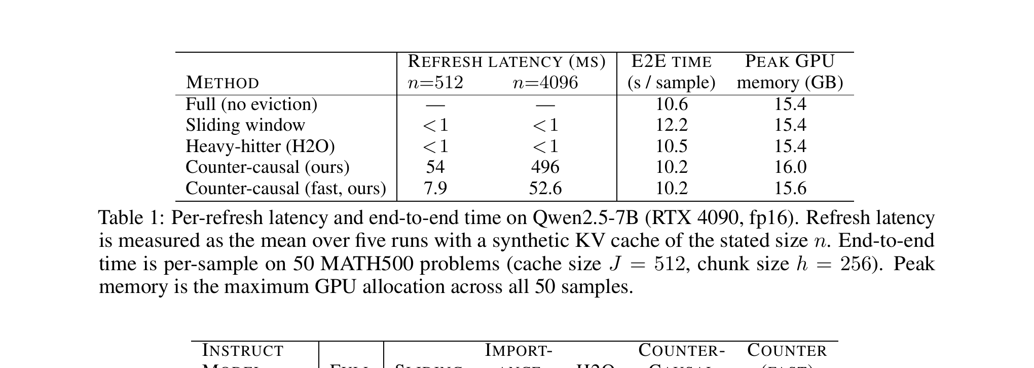
Running the full counter-causal pass through all $L$ transformer layers costs $O(Ln^2)$ per refresh, where $n$ is the current cache size — for a 28-layer model like Qwen2.5-7B, this genuinely adds meaningful latency (54ms at $n=512$, 496ms at $n=4096$, measured on an RTX 4090). The paper’s second contribution is a cheap approximation:

Idea: restrict the counter-causal computation to only the last transformer layer, using the hidden activations $H^{(L-1)}$ that would normally feed into that last layer during the ordinary causal forward pass — which are recorded (essentially for free, as a side effect) during the normal causal pass and stored alongside the cache. During a refresh cycle, fresh queries are computed from these stored $H^{(L-1)}$ activations (with RoPE applied at the original position IDs), a counter-causal mask is applied, and the layer’s standard output processing yields logits — but now costing $O(n^2)$ for one layer, not $O(Ln^2)$ for all $L$.

Why this works reasonably well, and where it should fail. The intuition is that the last transformer layer’s representations are already highly contextualized — by the time information reaches the final layer, a great deal of the earlier layers’ contextual mixing has already happened, so a single-layer counter-causal pass over near-final-layer activations captures much of what a full multi-layer counter-causal pass would. The measured cost is real: this reduces refresh latency by 7-9x (7.9ms vs 54ms at $n=512$; 52.6ms vs 496ms at $n=4096$) at only a small accuracy cost (e.g., 73.6% vs 74.4% on MATH500 with Qwen2.5-7B). The tradeoff is an extra memory cost: storing $H^{(L-1)}$ for every cached token costs roughly 12% of the KV cache’s own memory budget for Qwen2.5-7B (and falls to about 5% for the larger Qwen2.5-14B, since the hidden dimension grows more slowly than cache size relative to model capacity in this comparison). Interestingly, the paper’s own experiments show the fast approximation sometimes outperforms the full method on some long-context benchmarks (Section 4.4) — a genuinely surprising result the paper does not fully explain, which I flag as worth digging into (see Section 8).

3.4 Why the boundary condition and chunking interact

One subtlety worth making explicit: the last-token-always-kept rule (Section 3.2, Step 5) and the chunked refresh design (scoring every $h$ tokens rather than continuously) interact in a way the paper does not spell out in detail but that is worth tracing through. At the moment a refresh cycle fires, the most recent token in the current chunk has no future context within that chunk and is automatically assigned maximum surprise. But every other token in that same chunk does have some future context — namely, the other, more-recent tokens within the same $h$-token chunk — even though none of those chunk-local tokens will have had time to accumulate much “future” context yet, since the chunk has only just finished filling. This means tokens near the end of a chunk are systematically scored with less future context available than tokens near the beginning of a chunk. In practice this should bias the method slightly toward retaining recently-added tokens more than a hypothetical “infinite future context” version of counter-causal surprise would, which is arguably a benign bias (it pushes gently in the same direction as a recency prior, which is a reasonable inductive bias for language) but it is a real approximation gap between the idealized definition in Equation 1 (conditioning on all of $x_{i+1:t}$) and what the chunked, periodically-refreshed implementation actually computes at any given refresh call, since a token’s surprise score is only ever recomputed relative to whatever future context exists at refresh time, not updated continuously as more future context accumulates between refreshes.

4. Algorithms, spelled out step by step

The paper gives clean pseudocode for the three pieces of the system: the overall driver loop, the per-token inference step, and the memory refresh step.

Algorithm 1: Overall driver loop (pre-fill + decode)

1: function CacheManagedInference(x_1:T, J, h)      # Prompt, Cache Size, Chunk Size
2:     initialize buffers K, V, and memory M = (K', V')       # empty
3:     for t = 1, ..., T-1 do                                  # Pre-fill phase
4:         _ = DoInference(x_t)                                # process prompt token
5:         if t mod h == 0 then
6:             DoMemRefresh()                                  # periodic eviction decision
7:         end if
8:     end for
9:
10:    for t = T, ..., max_tokens do                            # Decode phase
11:        x_{t+1} = DoInference(x_t)                           # generate next token
12:        if t mod h == 0 then
13:            DoMemRefresh()                                   # periodic eviction decision
14:        end if
15:    end for
16: end function

Line-by-line reading: lines 3-8 handle the prompt (pre-fill), where every input token is processed but no sampling is needed; lines 10-15 handle generation (decode), where each new token is sampled autoregressively and fed back in. In both phases, exactly the same refresh trigger fires every $h$ tokens — this uniformity is a deliberate design choice: it means the same eviction machinery handles both a long input prompt and a long generated chain-of-thought without any special-casing.

Algorithm 2: Per-token inference step

1: function DoInference(x_t)
2:     compute queries, keys, values: q_t, k_t, v_t = f(x_t)
3:     K <- K + k_t                                    # append to recent-history buffer
4:     V <- V + v_t
5:     X <- X + x_t                                     # remember the token itself
6:     x~_t ~ P(x~ | q_t, K' + K, V' + V)               # sample next token via full attention
7:     return x~_t
8: end function

The key line here is line 6: attention for actually generating output always runs over the full concatenation of persistent memory ($K', V'$) and recent history ($K, V$) — eviction never affects the quality of any single generation step, only what survives into the next refresh cycle. Line 5 quietly introduces buffer $X$, which stores the raw token IDs (not just their key/value projections) — this is needed later because computing counter-causal surprise requires knowing the actual token identity $x_i$ whose logit you are scoring, and the memory overhead of storing integer token IDs is negligible next to the key/value tensors themselves.

Algorithm 3: Memory refresh step

1: function DoMemRefresh()
2:     for t = 1, ..., J+h do
3:         s_t = 1 - P(X_t | X_{t+1:J+h})       # counter-causal surprise, Eq. 1
4:     end for
5:     sigma = argsort(s_1, ..., s_{J+h})        # sort largest-surprise first
6:     K' <- (K' + K)[sigma[1:J]]                # keep the J highest-surprise entries
7:     V' <- (V' + V)[sigma[1:J]]
8:     X <- X[sigma[1:J]]
9:     clear K and V
10: end function

Step by step: line 2-4 scores every one of the up to $J+h$ candidate tokens (the $J$ already in persistent memory plus the $h$ new ones from the current chunk) using the counter-causal pass described in Section 3.2. Line 5 sorts by descending surprise. Lines 6-8 keep only the top $J$ by surprise and discard the rest, maintaining a strict one-to-one correspondence between the surviving tokens in $X$ and their key/value pairs. Line 9 clears the recent-history buffer, ready for the next chunk. Crucially, this entire refresh operation processes tokens in batch — even during the decode phase, where inference itself is one-token-at-a-time, the refresh scoring is not, because no new token needs to be sampled during a refresh; it is a pure batched forward pass over already-known tokens.

A worked toy example. Suppose the cache (after some generation) holds the phrase “…the capital of France is Paris and it is located on the Seine river…”. Consider evicting either “Paris” or “river”: scoring “river” counter-causally, the model sees “…is Paris and it is located on the Seine ___…” — a strong context clue (“Seine” almost always precedes “river” in this construction) makes “river” highly predictable from its future-less context; wait — actually the counter-causal direction means “river” is scored using only what follows it, which in this toy sentence might be nothing or an unrelated clause, so this example is more subtle than it first appears; the intuition holds better for “Paris”: if the sentence continues ”…Paris, home of the Eiffel Tower, sits on the Seine…”, then even without seeing the word “Paris” directly, a model conditioning only on “home of the Eiffel Tower, sits on the Seine” could infer with high confidence that the missing city is Paris — hence low surprise, safe to evict, because the future context alone already pins down the fact. Conversely, a token like a specific patient ID number in a clinical record, which nothing later in the document restates or implies, would receive high surprise under any future context and would be protected.

5. Design choices, discussed: why, what’s the alternative, where does it break

Design choice 1 — token-level scoring (not phrase or sentence level). Why it works: it slots directly into the existing per-token KV cache data structure with no architectural change — every cached key/value pair already corresponds to exactly one token, so a token-level score requires no new bookkeeping. The obvious alternative: score at a coarser granularity (phrases, sentences, or semantic chunks), which could better capture cases where information is distributed across several adjacent tokens rather than concentrated in one. Where it fails: the paper explicitly flags this as a limitation — an individual token that is easily predictable in isolation (e.g., a common word in a multi-word named entity) may receive low surprise and get evicted even though it is part of an exact-match phrase that a downstream retrieval-style task needs verbatim. This is a genuine boundary condition: counter-causal surprise measures information content, not verbatim retrievability, and the two diverge exactly when partial-but-predictable pieces of a string are individually low-surprise but collectively load-bearing for exact string match.

Design choice 2 — reusing cached K/V instead of recomputing with a genuinely retrained reverse model. Why it works: it is training-free and works with any existing pretrained autoregressive model off the shelf — no fine-tuning, no auxiliary reverse LM, no data collection. This is a major practical advantage over approaches like NAMMs (Section 6) that require training a separate eviction-scoring network. The obvious alternative: actually train a bidirectional or reverse-direction model to compute $P(x_i \mid x_{i+1:t})$ exactly. Where it fails: because the model was never trained on counter-causal masks, the approximation quality is unverified in any formal sense — the paper is candid that “neither the cached forward pass nor the single-layer proxy exactly models $P(x_i \mid x_{i+1:t})$.” It is a heuristic justified by strong empirical results, not a provably correct estimator, and its quality likely varies by model family and how much of the training corpus resembled bidirectional-style text (masked LM pretraining objectives, if a checkpoint had any, might make this proxy more or less faithful — the paper does not investigate this).

Design choice 3 — chunked refresh (score every $h$ tokens) rather than continuous per-token refresh. Why it works: computing counter-causal surprise for a token requires it to have some future context (otherwise, per the boundary rule, it defaults to maximum surprise and is trivially kept) — so refreshing too frequently would waste computation scoring tokens that have barely any future context yet, while refreshing infrequently amortizes the (non-trivial) cost of the scoring pass over many decode steps. The obvious alternative: refresh after every single generated token, giving the most up-to-date eviction decisions at maximum computational cost. Where it fails: larger $h$ means the transient recent-history buffer $K, V$ can itself temporarily exceed the intended memory budget $J$ by up to $h$ tokens between refreshes — this is a real, if modest, headroom cost that has to be budgeted for in a production memory allocator, and the paper does not discuss how sensitive results are to the specific choice of $h$ relative to $J$ (they use $h = J/4$ throughout, but do not ablate this ratio).

Design choice 4 — freezing the system prompt as un-evictable “sink” slots. Why it works: the paper follows prior work (StreamingLLM’s attention sink observation) in reserving a small fixed number of memory slots for the task’s system prompt, which are never subject to eviction scoring at all. This avoids the pathological case where counter-causal scoring (or any other scoring rule) might accidentally evict task-defining instructions because they happen to be “predictable” from later context, even though losing them would derail the entire generation. The obvious alternative: let the system prompt compete for slots on equal footing with everything else, trusting the scoring rule to protect it if it is truly important. Where it fails: baking in a fixed sink allocation is itself a manual design decision that assumes you know, structurally, which tokens are “system prompt” versus “task context” — this works cleanly in the paper’s benchmark setup (where this boundary is well-defined) but is a less clean abstraction in settings with more fluid, multi-turn, tool-augmented context where “what counts as unevictable” is not obviously fixed at the start.

6. Experimental setup and results, examined closely

The paper evaluates on two open-weight model families — Qwen2.5 (3B/7B/14B Instruct) and LLaMA-3.1-8B-Instruct — across four benchmark tasks chosen specifically to stress-test both pre-fill-heavy eviction (long input, short output: LongHealth, Qasper, LoCoMo) and decode-heavy eviction (short input, very long generated chain-of-thought: MATH500, AIME). This dual-phase testing matters: a method that only works well when evicting from a long static prompt but breaks down when evicting from a growing, self-generated reasoning trace would be a much weaker result.

Five eviction strategies are compared: Full (no eviction, the reference ceiling), Sliding window (pure recency, FIFO), Importance (a simplified heavy-hitter/TOVA-like baseline using last-layer attention), H2O (the canonical accumulated-attention heavy-hitter oracle), and the paper’s own Counter-causal and Counter-causal (fast).

Efficiency (Table 1). On Qwen2.5-7B (RTX 4090, fp16), the full $L$-layer counter-causal pass costs 54ms at cache size $n=512$ and 496ms at $n=4096$, versus under 1ms for the attention-based baselines — a real, non-trivial overhead. The fast single-layer approximation cuts this to 7.9ms and 52.6ms respectively, a 7-9x speedup. Critically, end-to-end per-sample time on MATH500 (10.2s for both counter-causal variants) is essentially tied with the no-eviction baseline (10.6s) despite this refresh overhead, because a smaller cache also means cheaper per-token attention during the long decode phase — the refresh cost is offset by savings elsewhere. Peak GPU memory is only modestly higher for the counter-causal methods (16.0GB full / 15.6GB fast, versus 15.4GB baseline), the fast variant’s extra cost coming from storing the $H^{(L-1)}$ activation buffer.

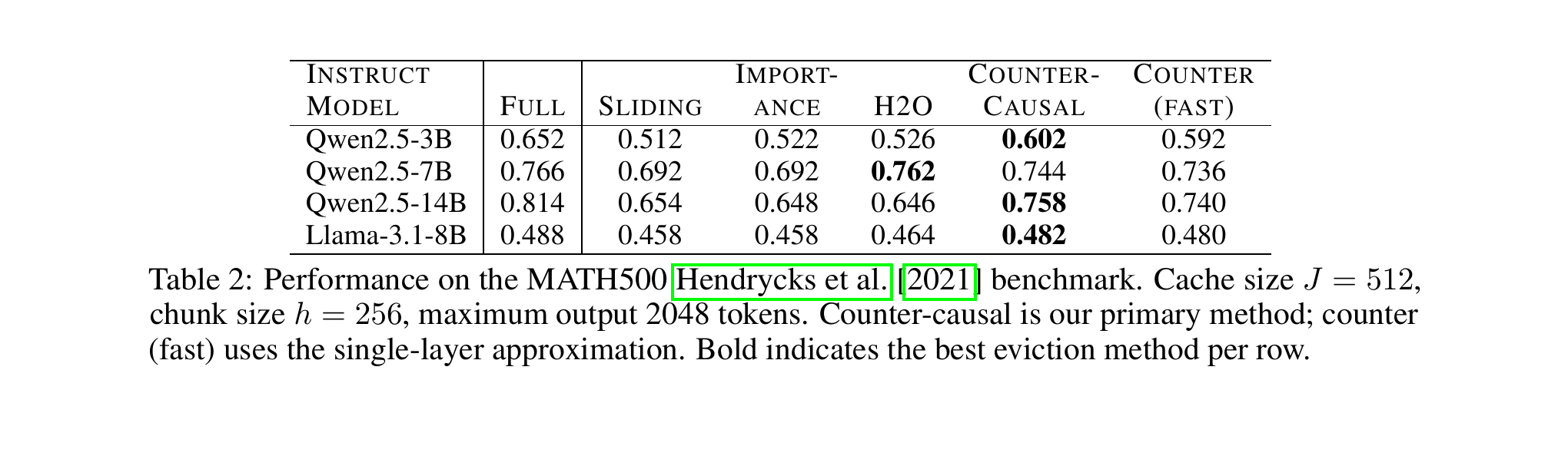
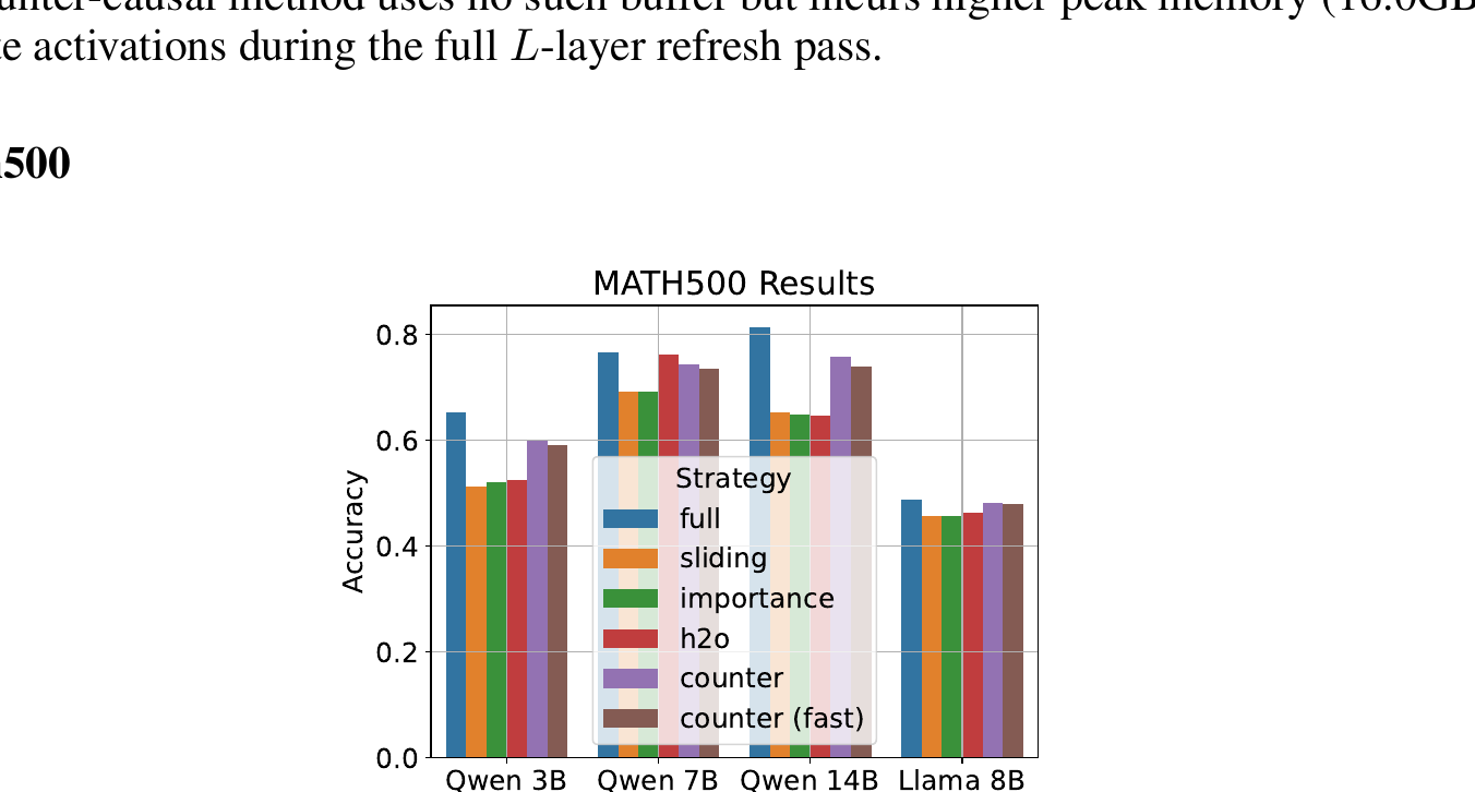
MATH500 (Table 2, Figure 2). With a cache budget $J=512$ (chunk size $h=256$), counter-causal is the best eviction method on 3 of 4 models: 60.2% (Qwen2.5-3B), 74.4% (Qwen2.5-7B, though H2O edges it out at 76.2% on this one model), and 75.8% (Qwen2.5-14B). On LLaMA-3.1-8B it achieves 48.2%, nearly matching the 48.8% no-eviction ceiling and again the best eviction method tested. The fast approximation trails the full method by roughly 1-2 percentage points across models while being 7-9x cheaper per refresh — a genuinely favorable tradeoff for most deployment scenarios.

The cache-content visualization (Figure 4) is the single most illuminating figure in the paper. For one MATH500 problem, the authors visualize which generation-timestep tokens survive each refresh cycle, for sliding window, importance sampling, and counter-causal, with rows showing successive refresh cycles and columns showing cache entries colored by their original generation timestep.

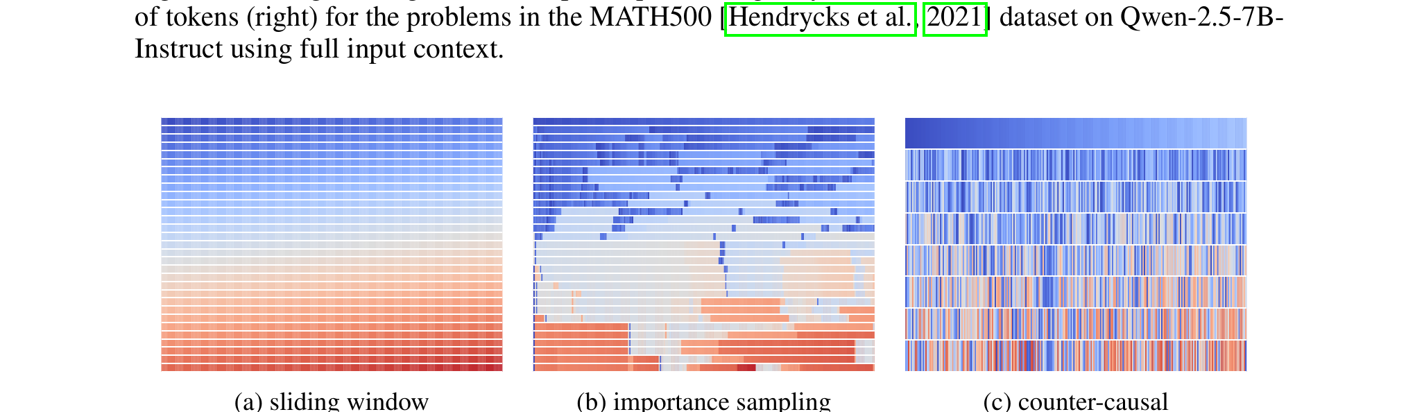
This figure is worth staring at for a while. Panel (b), the importance-sampling / heavy-hitter-style method, shows exactly the self-reinforcing bias the paper’s motivation section warns about: a handful of early spans (visible as persistent vertical striping across many rows) keep winning the retention competition round after round, crowding out anything new. Panel (c), counter-causal, shows a much finer-grained, more evenly distributed retention pattern across the whole timestep range — consistent with a scoring rule that re-evaluates relevance from scratch at each cycle rather than accumulating momentum. The caption also notes counter-causal produced a shorter correct answer on this specific problem than the other strategies, which the authors interpret as the model reasoning more efficiently when the cache holds more genuinely useful (rather than merely historically over-attended) content — though I would flag this specific single-problem anecdote as illustrative rather than a load-bearing empirical claim (see critical analysis, Section 8).

AIME, thinking-mode reasoning (Table 3). This is the paper’s most decode-heavy stress test: Qwen3-8B in thinking mode, generating up to 16,384 tokens of <think>...</think> reasoning before a final boxed answer, with a tight cache budget ($J=4096$, i.e., 25% retention at the maximum length). All methods degrade substantially under this pressure — the frequent evictions disrupt the reasoning chain badly enough that a meaningful fraction of runs never even close the </think> tag within the token budget (the pred=None row). Counter-causal achieves 36.7% accuracy, clearly the best eviction method (versus 26.7% sliding, 14.4% importance, 33.3% H2O), and also has among the lower pred=None rates (57%, versus 83% for importance sampling) — suggesting it disrupts the reasoning chain’s internal coherence less than attention-based alternatives, even though it still falls well short of the 50.0% unconstrained-cache ceiling.

LongHealth, Qasper, LoCoMo (Figure 5). These three tasks sweep across a range of cache sizes and stress pre-fill-phase eviction from long, information-dense input documents (clinical records, scientific papers, and 300-turn multi-session conversations, respectively). The paper’s most striking qualitative finding here concerns LoCoMo: H2O specifically struggles at small cache budgets, and the authors diagnose two concrete failure modes by manually inspecting outputs — (1) the model’s answer literally repeats the input question verbatim, indicating total loss of relevant conversational context, and (2) the model injects irrelevant image captions from earlier in the conversation, because image-caption tokens attracted disproportionate cumulative attention from many nearby tokens and thus survived eviction at the expense of factual content asked about later. Counter-causal avoids both failure modes because a rarely-mentioned fact that cannot be inferred from later context receives high surprise regardless of how much attention it originally attracted — exactly the property the method was designed to have.

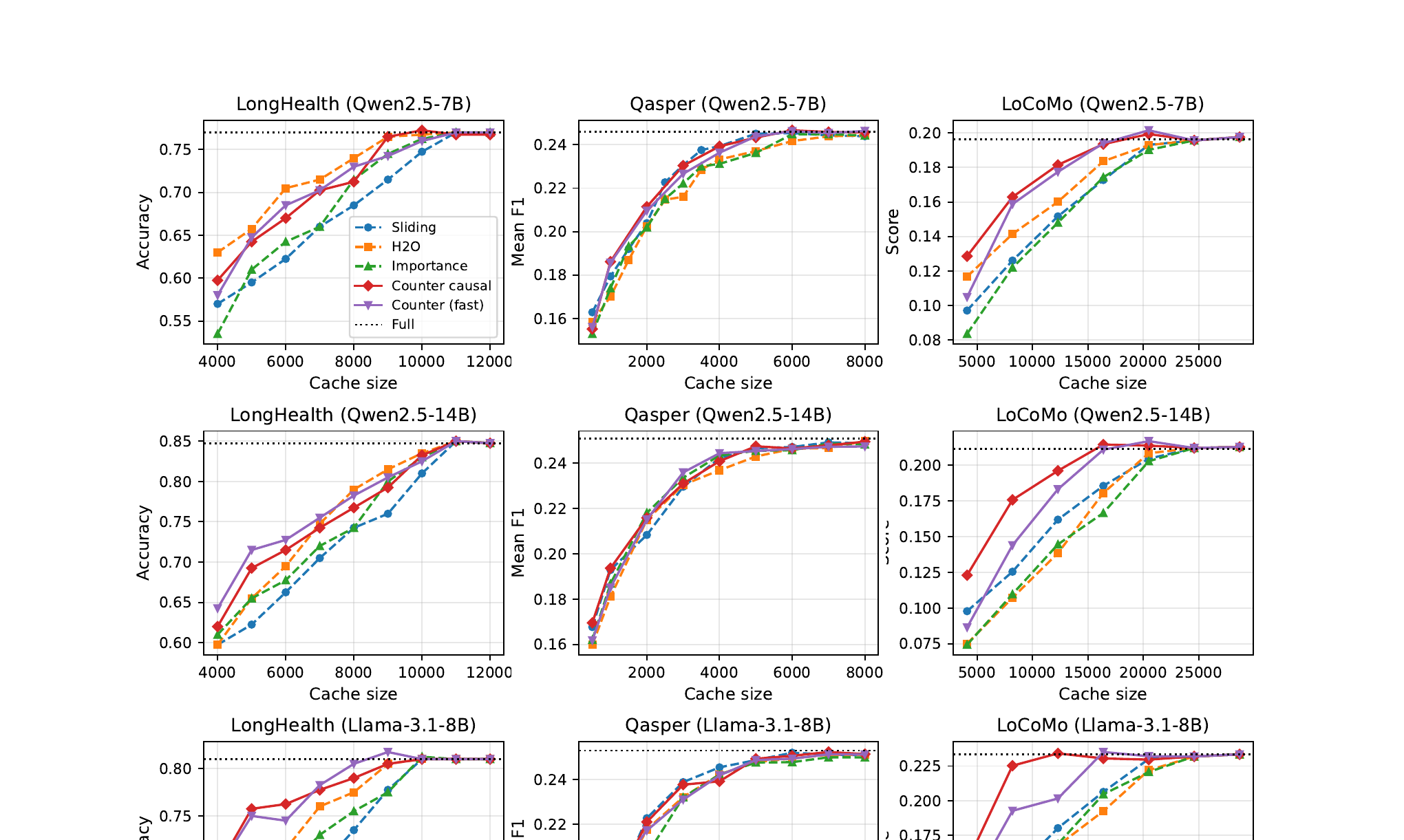
Notably, on Qasper specifically, all five strategies perform almost identically regardless of cache size — the paper does not dwell on why, but a plausible explanation (not stated explicitly by the authors) is that Qasper’s question-answering format may not require synthesizing information spread thinly across the document the way LoCoMo’s multi-hop conversational questions or LongHealth’s clinical cross-referencing do, making it a weaker discriminator between eviction strategies.

7. Limitations, as stated by the authors

The paper is candid about several limitations. First, the full counter-causal method genuinely costs extra compute — $O(Ln^2)$ per refresh, “roughly doubling inference cost during pre-fill when refreshes are frequent,” though the paper argues this cost is largely amortized and negligible during the decode phase, where it operates on a batch of already-cached tokens rather than the one-token-at-a-time cost of ordinary decoding. Second, counter-causal surprise is explicitly acknowledged as an approximation: “neither the cached forward pass nor the single-layer proxy exactly models $P(x_i \mid x_{i+1:t})$” — there is no formal guarantee the surprise score tracks the true reverse-conditional probability, only strong empirical support that it behaves usefully in practice. Third, and most substantively, the authors flag the token-level scoring granularity itself as a limitation: individual tokens that are easily predictable in isolation can be evicted even when they are part of a larger span needed verbatim for exact-match retrieval tasks, and they suggest phrase-or-sentence-level scoring, or hybrid approaches mixing counter-causal scoring with recency- or retrieval-aware signals, as future work.

8. Critical analysis

Weaknesses and flaws specific to this paper. The efficiency comparison in Table 1, while honest about the full method’s latency cost, somewhat undersells how that cost scales: the reported 496ms-per-refresh at $n=4096$ for the full method is already substantial, and for a truly long-context deployment (say 128K tokens, an increasingly common target for “long context” LLM serving), the $O(Ln^2)$ scaling means refresh cost grows quadratically in cache size — the paper’s own experiments cap out at $n=24576$ tokens for LoCoMo, and it is not demonstrated (nor argued theoretically beyond the stated big-O) how the full method would behave at the 100K+ token contexts that are increasingly the actual target market for KV-cache compression research. The fast approximation mitigates this to $O(n^2)$, but that is still quadratic, not linear, in cache size — a genuinely important scaling ceiling that is understated relative to how central “efficiency” is to the paper’s stated motivation.

Limitations the authors understate or omit. The paper compares against H2O, TOVA-style “importance,” and sliding window, but explicitly declines to include PyramidKV or Ada-KV as baselines, arguing (correctly, in principle) that these are “orthogonal” layer-budget-allocation strategies rather than alternative scoring rules, and noting they share H2O’s underlying attention-based signal and thus “the same self-reinforcing bias.” This is a reasonable theoretical argument, but it is also a convenient one: PyramidKV and Ada-KV are precisely the strongest recent attention-based baselines, and if the self-reinforcing-bias critique is as fundamental as the paper claims, empirically demonstrating that these more sophisticated attention-based methods still underperform counter-causal (rather than arguing by analogy that they should) would have been a stronger, more falsifiable piece of evidence. As written, the comparison set is dominated by comparatively older or simpler baselines (H2O is from 2023; sliding window and basic importance sampling are essentially heuristics), which somewhat inflates how impressive the margin looks. Additionally, the paper reports the “fast approximation sometimes outperforming the full method” (Section 4.4, LongHealth) without any attempt at explanation — this is either noise (a single-seed, greedy-decoding result with no error bars reported anywhere in the paper) or a genuinely interesting phenomenon (perhaps the full method’s extra layers of counter-causal computation introduce their own approximation noise relative to the true reverse-conditional, in a way the single-layer method happens to avoid) — but the paper does not investigate which, and given every experiment uses a single greedy rollout with no repeated trials or confidence intervals reported anywhere, some fraction of the reported differences (including this one) could plausibly be within noise.

Concrete, specific improvement suggestions. (1) Report variance or multiple seeds/rollouts, even a small number, for at least the headline MATH500 and AIME numbers — greedy decoding with a single rollout per problem, with differences as small as 1-2 percentage points between methods (e.g., counter-causal’s 74.4% vs H2O’s 76.2% on Qwen2.5-7B MATH500) being used to declare a “win” or “loss,” is a genuinely weak statistical basis for the paper’s comparative claims. (2) Directly benchmark against PyramidKV and/or Ada-KV rather than only arguing by analogy that they share H2O’s bias — this is a testable claim the paper is well-positioned to make but does not. (3) Report wall-clock refresh cost scaling empirically beyond $n=4096$ (e.g., at 32K, 64K, 128K) rather than relying solely on the stated asymptotic complexity, since real deployments increasingly target these longer regimes and quadratic-in-$n$ costs can dominate unexpectedly at scale. (4) Investigate and report why the fast approximation sometimes beats the full method — this is scientifically the most interesting anomaly in the paper’s own results and is currently left as an unexplained footnote-level observation. (5) The paper’s proposed future direction of phrase/sentence-level scoring is promising but under-specified — a natural, testable first step would be simply averaging counter-causal surprise scores within a small fixed-size sliding window of adjacent tokens before ranking, which would require no architectural change and could be evaluated immediately with the existing experimental setup, rather than left as an open suggestion.

8b. A note on comparing against a moving research frontier

It is worth situating this paper’s July 2026 submission date against how fast KV-cache eviction research is moving. The comparisons in this paper (H2O 2023, TOVA-style importance sampling, sliding window) represent the foundational generation of eviction methods, not the current state of the art as of the paper’s own related-work section, which itself cites PyramidKV (2024), Ada-KV (2024), KVzip (2025), and NAMMs (2025) as more recent and more sophisticated alternatives — yet none of these appear as empirical baselines in Section 4. This is a common and understandable practical constraint (each additional baseline requires reproducing someone else’s method faithfully, which is nontrivial engineering work), but it does mean a reader should calibrate their expectations: the paper convincingly demonstrates that counter-causal surprise beats the first wave of attention-based eviction, and offers a plausible, well-argued theoretical reason why it should also beat the second wave (since they share the same underlying attention-based signal), but this second claim remains an inference from the paper’s own theoretical argument rather than a directly measured result. A careful reader evaluating whether to adopt this method in place of, say, an already-deployed PyramidKV pipeline, would be well served by running this comparison themselves before committing, especially given how close some of the reported margins are (Section 8).

9. Reproducibility notes

The authors state reference code is available at https://github.com/metacognitionai/counter_causal. The paper reports precise hyperparameters for each experiment (cache size $J$, chunk size $h$, maximum output tokens) directly in table captions, which is good practice and makes the headline numbers reproducible in principle. Hardware is specified precisely (NVIDIA H100 NVL 94GB for accuracy experiments, RTX 4090 for efficiency benchmarks; Python 3.11/3.12, PyTorch 2.10.0+cu128), and system prompts used for each benchmark task are included in a paper appendix. The main reproducibility gap, as noted above, is the absence of any stated random seed policy or repeated-trial protocol — greedy decoding is deterministic given a fixed model and prompt, so results should in principle reproduce exactly given the same code and model checkpoint, but this also means the reported numbers carry no information about run-to-run variance, which matters more the closer two methods’ reported scores are to each other.

10. Where this fits in the broader KV-cache eviction landscape

Counter-causal surprise is best understood as attacking the scoring function axis of KV-cache eviction, orthogonal to two other axes that recent work has explored: budget allocation (PyramidKV, Ada-KV — how much cache to give each layer/head, holding the scoring rule fixed) and representation compression (quantization methods like KVQuant, or spectral/low-rank summarization methods like the LOCKS paper reviewed on this blog last week — how compactly to store what you keep, holding the eviction decision itself fixed). In principle, these are compatible: nothing prevents combining counter-causal scoring with per-layer budget allocation and quantized storage of surviving entries, and the paper explicitly notes PyramidKV’s layer allocation strategy as “orthogonal … and could in principle be combined with counter-causal eviction in future work.” This composability is, I think, the paper’s most practically important framing contribution even beyond the specific scoring rule: it correctly identifies which existing techniques it competes with versus which it complements, and a production KV-cache manager combining all three axes (a smarter scoring rule, adaptive per-layer budgets, and quantized storage) is a very plausible next step for the field.

11. Practical takeaways

If you are building or tuning a KV-cache eviction system today, the practical decision this paper offers is straightforward: if your workload has occasional rare, load-bearing facts that must survive long stretches of generation (clinical QA, long multi-session dialogue memory, retrieval-style tasks over long documents), attention-based heavy-hitter methods carry a real, empirically demonstrated risk of losing exactly that information due to self-reinforcing bias, and counter-causal scoring is a training-free drop-in alternative worth trying. If your latency budget cannot absorb the full method’s refresh cost, the single-layer fast approximation gives most of the accuracy benefit at a fraction of the cost, at the price of a modest additional memory buffer for storing penultimate-layer activations. If your task instead depends on exact verbatim retrieval of short but individually-predictable token spans (e.g., precise phrase matching), be aware of the token-level scoring limitation the authors themselves flag, and consider that this specific failure mode has not yet been empirically demonstrated or fixed in this paper — it is a known open gap, not a solved edge case.

11b. A simple decision framework

Given the tradeoffs unpacked above, here is a compact way to decide which eviction strategy to reach for first, based on what matters most for a given deployment:

1. Is your workload dominated by very long, mostly-redundant generated text (e.g., verbose chain-of-thought) where a handful of facts stated once must survive to the end? If yes, counter-causal (or its fast variant) is the strongest candidate demonstrated in this paper — both the MATH500 and AIME results show it best preserves reasoning coherence under aggressive eviction.
2. Is your latency budget extremely tight and every millisecond of refresh overhead matters (e.g., interactive low-latency serving with frequent small refresh cycles)? Prefer the fast single-layer approximation over the full method; the accuracy cost is consistently small (roughly 1-2 points) relative to the 7-9x latency win, and in some regimes (Section 6, LongHealth) the fast variant is not even worse.
3. Does your task require exact verbatim retrieval of short, individually-predictable spans (e.g., exact phrase matching, ID numbers embedded in predictable surrounding text)? Be cautious — this is the one failure mode the authors themselves identify and have not solved; a hybrid scheme mixing counter-causal scoring with a recency or exact-match-aware signal is likely necessary, but is not evaluated in this paper.
4. Is your primary bottleneck cache capacity at very long context lengths (64K-128K+) where refresh cost may start to dominate due to quadratic scaling? Treat this paper’s efficiency numbers (measured up to $n=4096$) as encouraging but not yet validated at your target scale — benchmark the actual refresh latency at your real cache sizes before committing, since neither variant’s cost is linear in $n$.
5. Do you already have a per-layer budget allocator (PyramidKV-style) or a quantized storage backend in production? Counter-causal scoring is designed to be orthogonal and composable with both — there is no architectural reason it cannot replace just the scoring component of an existing pipeline while keeping the rest unchanged.

12. Conclusion

This paper’s contribution is conceptually narrow but well-executed: a single new scoring function for an eviction decision that every long-context LLM serving system already has to make. What makes it worth reading is not algorithmic novelty in the mechanical sense — reusing cached K/V with a flipped attention mask is a simple idea — but the clarity of the diagnostic argument (self-reinforcing bias in attention-based scoring, demonstrated concretely via the LoCoMo failure-mode analysis and the cache-content visualization in Figure 4) paired with a genuinely training-free, drop-in-compatible fix. The empirical wins are real but modest in magnitude on some benchmarks, the statistical rigor is thinner than the strength of the claims would ideally warrant, and the quadratic cost scaling of even the fast approximation is a ceiling worth watching as context lengths keep growing — but the core idea, that predictability from the future is a more principled retention signal than attention received from the past, is a genuinely useful lens that I expect other KV-cache management work to build on.