DynaCalKV: Rethinking Fixed Head Grouping in Low-Rank KV Cache Compression

Review date: 2026-07-31 Author: Zhongzhu Zhou Paper reviewed: DynaCalKV: Key-Value Cache Compression via Head Grouping and Adaptive Rank Allocation Paper authors: Tan T. Nguyen, Quan V. Dang arXiv: 2607.24331 Venue/Status: Preprint, July 27, 2026

1. Why this paper, and what problem is it actually solving

Every time an LLM generates a new token, it has to attend back over every previously generated token’s Key and Value vectors. Storing those vectors — the “KV cache” — is what makes autoregressive decoding fast (you never recompute attention for old tokens), but it is also what makes long-context serving expensive: the cache grows linearly with sequence length, and at 32K+ tokens it can dwarf the memory footprint of the model’s own weights. A huge amount of systems research over the last two years has gone into shrinking this cache without hurting model quality, and the field has split into three broad families: quantization (store KV in fewer bits, e.g. KIVI, KVQuant), token eviction (throw away KV entries judged unimportant, e.g. H2O, SnapKV, CAKE), and low-rank compression (project KV into a smaller latent space via SVD or a learned linear map, e.g. Palu, LoRC, MatryoshkaKV, Eigen-Attention).

DynaCalKV sits in the third family, and specifically improves on a 2025 method called ReCalKV, which itself builds on Palu. The paper’s core observation is narrow but genuinely useful: ReCalKV compresses the Key cache by first grouping attention heads (so that heads with similar behavior can share a single low-rank projection) and then applying SVD within each group — but it always uses a fixed group size of exactly 4 heads, regardless of how similar or dissimilar the heads in a given layer actually are. DynaCalKV asks the obvious follow-up question: what if we let the actual similarity structure of the heads decide how many groups there should be and how large each one is, instead of hard-coding “4 heads per group” everywhere? The answer, worked out carefully with a parameter-budget constraint so the comparison stays fair, is that dynamic grouping recovers meaningful additional compression on standard multi-head attention (MHA) models, but can backfire on architectures that are already head-sparse (grouped-query attention, GQA) under long-context evaluation. That asymmetric result — “works great here, actively hurts there, and here’s the mechanism why” — is what makes this a worthwhile six-page read even though the method itself is a fairly surgical modification of an existing pipeline.

If you already work with KV-cache compression, speculative decoding, or quantization, this paper is a clean case study in a recurring systems lesson: an “adaptive” version of a heuristic is not automatically better — it is only better when the thing you’re adapting to (head similarity, in this case) is actually informative for the architecture you’re applying it to.

Prerequisites: what you need to know before diving in

This paper assumes you are comfortable with the transformer attention mechanism and matrix factorization. Here is what to have in your head before Section 3.

Multi-head attention, GQA, and why head count matters here. In standard multi-head attention (MHA), every attention head has its own independent Key and Value projection, so a model with $h$ heads has $h$ distinct sets of Key/Value vectors to cache. Grouped-Query Attention (GQA) reduces KV-cache memory before any compression is even applied by sharing a single Key/Value head across a group of Query heads — so a GQA model might have, say, 32 Query heads but only 8 Key/Value heads. This paper’s central empirical finding hinges on this distinction: MHA models arrive with many independent, genuinely-cacheable Key heads to work with, while GQA models arrive already thinned out. Squeezing further structure out of 8 heads is a much riskier proposition than squeezing it out of 32.

Singular Value Decomposition (SVD) as a compression primitive. Any matrix $W \in \mathbb{R}^{m \times n}$ can be exactly factored as $W = U\Sigma V^\top$, where $U$ and $V$ are orthogonal and $\Sigma$ is diagonal with non-negative entries (the singular values) sorted in decreasing order. If you keep only the top $r \ll \min(m,n)$ singular values/vectors, you get the best possible rank-$r$ approximation $W \approx L R$ (in the Frobenius-norm sense) with $L = U_r \Sigma_r^{1/2}$, $R = \Sigma_r^{1/2} V_r^\top$. Applied to a Key or Value projection matrix, this means an activation $x$ that would normally need to be projected to a full $n$-dimensional Key/Value vector can instead be cached as a much smaller $r$-dimensional vector $z = xL$, and reconstructed (approximately) as $z R$ only when actually needed for attention. This is the mechanism every low-rank KV-cache paper — Palu, LoRC, ReCalKV, and now DynaCalKV — relies on.

Why you’d group heads before applying SVD. If you naively apply SVD to the entire Key projection matrix for a layer (all heads concatenated), you get one shared low-rank basis for all heads, which wastes capacity on heads that behave very differently from each other. If you apply SVD separately to every single head, you get maximum specificity but pay per-head overhead and lose the chance to share structure between heads that happen to behave almost identically (which is common — many attention heads learn redundant or near-duplicate patterns). Grouping heads by similarity and running one SVD per group is the middle ground: put similar heads together (they can share a low-rank basis cheaply) and keep dissimilar heads apart (so they don’t force a compromise basis on each other).

Centered Kernel Alignment (CKA). CKA is a similarity metric for comparing two sets of representations, originally popularized for comparing hidden layers across different neural networks. Given two centered feature matrices $X \in \mathbb{R}^{n \times d_x}$ and $Y \in \mathbb{R}^{n \times d_y}$ (same number of rows $n$, possibly different feature dimensions), linear CKA is:

$$\mathrm{CKA}(X, Y) = \frac{\lVert Y^\top X \rVert_F^2}{\lVert X^\top X \rVert_F \, \lVert Y^\top Y \rVert_F} \tag{1}$$

where $\lVert \cdot \rVert_F$ is the Frobenius norm. The score is bounded in $[0,1]$, with $1$ meaning the two representations are (up to rotation/scaling) identical, and $0$ meaning they are orthogonal/unrelated. In DynaCalKV, $X$ and $Y$ are the output representations of two different attention heads on the same calibration data, so $\mathrm{CKA}(X,Y)$ answers the question “how similar is head $i$‘s behavior to head $j$‘s behavior?” — the exact signal you need before deciding whether they belong in the same compression group.

Fisher Information for layer-wise budget allocation. Not every layer in a deep network is equally important to preserve exactly; some layers’ outputs matter much more to the final loss than others. Fisher Information gives a cheap, gradient-based proxy for “how sensitive is the loss to perturbing this layer’s parameters” — layers with higher Fisher Information get a bigger share of the compression budget (more rank kept), and layers with lower Fisher Information get compressed more aggressively. This paper inherits this allocation strategy directly from Palu rather than inventing a new one, which is worth flagging up front since it means the layer-level budgeting is not actually this paper’s contribution — the paper’s contribution is entirely about how the within-layer, within-Key-cache budget gets distributed across head groups.

A quick numeric intuition for why GQA changes the calculus. Consider a hypothetical 32-head MHA model versus an 8-Key-head GQA model serving the same total number of Query heads (32). In the MHA case, DynaCalKV’s clustering has 32 candidate heads to search for redundancy among — plenty of room to find, say, four clusters of 8 near-duplicate heads each and compress aggressively. In the GQA case, there are only 8 Key heads to begin with, and GQA’s own design already assumes each of those 8 heads carries meaningfully distinct information (that’s why the model’s designers didn’t shrink further to, say, 2 or 4 Key heads in the first place). Asking a clustering algorithm to find further redundancy among an already-curated set of 8 heads is asking it to manufacture structure that may simply not exist — and if it merges heads anyway (because the algorithm doesn’t know the heads were already curated to be non-redundant), it will discard real information rather than actual redundancy. This is the intuitive core of the paper’s central finding, independent of the specific CKA/energy/greedy machinery.

With this vocabulary, the rest of the paper reads as: “take ReCalKV’s pipeline, replace its fixed-size head grouping with a similarity-driven adaptive one, and see where that helps and where it hurts.”

2. Architecture overview: where DynaCalKV sits in the pipeline

DynaCalKV is not a new end-to-end system; it is a drop-in replacement for one stage of an existing compression pipeline (Palu → ReCalKV). The overall offline compression flow, once you situate DynaCalKV inside it, looks like this:

flowchart TD
    A["Pretrained LLM checkpoint"] --> B["Per-layer Fisher Information<br/>scoring on calibration data<br/>(inherited from Palu)"]
    B --> C["Layer-wise rank budget r<br/>allocated across all layers"]
    C --> D{"Key projection W(k)<br/>or Value projection W(v)?"}
    D -- "Key W(k)" --> E["DynaCalKV: CKA similarity matrix S<br/>+ adaptive clustering + rank allocation<br/>(Algorithm 1)"]
    D -- "Value W(v)" --> F["ReCalKV-style whole-matrix SVD<br/>+ calibration-data refinement<br/>(closed-form L_v, R_v update)"]
    E --> G["Compressed Key cache:<br/>per-group low-rank factors {L_i, R_i}"]
    F --> H["Compressed Value cache:<br/>single low-rank factor pair (L_v, R_v)"]
    G --> I["Deployed model: cache z = xL<br/>instead of full K, reconstruct zR at attention time"]
    H --> I

Figure 1 (self-drawn, Mermaid): DynaCalKV’s place in the compression pipeline. Only the Key-cache branch (left) is DynaCalKV’s contribution; the Value-cache branch (right) is inherited unchanged from ReCalKV, and the layer-level budget allocation (top) is inherited unchanged from Palu.

This scoping matters for reading the paper correctly: DynaCalKV is a strict subset modification. It touches only how heads are grouped and how rank is distributed within the Key cache of a single layer. It does not touch cross-layer budget allocation, and it does not touch the Value cache compression strategy at all — both of those are carried over from prior work. This is a deliberate, honest scoping choice by the authors (they say so explicitly), and it is also why the empirical section can isolate the effect cleanly: any change in results traces back to exactly one design decision.

Data flow: from a Key projection matrix to a compressed cache

flowchart LR
    W["Key projection matrix<br/>W(k) in R^(m x n)<br/>n = h heads x d_h each"] --> S["Pairwise CKA similarity<br/>matrix S in R^(h x h)"]
    S --> Cl["Agglomerative clustering<br/>into K groups (K varies)"]
    Cl --> En["Per-group energy<br/>(sum of squared singular values)"]
    En --> R0["Initial rank r_i proportional<br/>to group energy"]
    R0 --> Adj["Greedy rank-reduction pass:<br/>shrink cheapest group first<br/>until parameter budget met"]
    Adj --> Dec["Per-group SVD:<br/>W_i approx L_i R_i"]
    Dec --> Out["Compressed Key cache<br/>{L_i, R_i} for all groups"]

Figure 2 (self-drawn, Mermaid): The full Key-compression data flow for a single layer, corresponding to Algorithm 1 in the paper. Every arrow in this diagram happens once, offline, during the calibration/compression stage — none of it adds runtime overhead during inference, since only the resulting compact factors $\{L_i, R_i\}$ are ever used at serving time.

The object at the center of this whole method is the similarity matrix $S \in \mathbb{R}^{h \times h}$, where $h$ is the number of attention heads in a layer and each entry $S_{i,j} = \mathrm{CKA}(\text{head}_i, \text{head}_j)$. Everything downstream — how many groups form, which heads end up together, how much rank each group gets — is a function of this one matrix. That is both the method’s elegance and its Achilles’ heel: if $S$ doesn’t carry a clean cluster structure (which, as we’ll see, is exactly what happens for high-head-dimension architectures), the whole downstream pipeline degrades gracefully into something close to “one singleton group per head,” which is not obviously better than the ReCalKV baseline it’s trying to beat.

3. Method details: from ReCalKV’s fixed grouping to DynaCalKV’s adaptive one

3.1 The ReCalKV baseline, formalized

Given a Key projection matrix $W^{(k)} \in \mathbb{R}^{m \times n}$ where $n = h \cdot d_h$ ($h$ heads, each of dimension $d_h$), and a total rank budget $r$ for this matrix, ReCalKV partitions the $h$ heads into groups of a fixed size (4 heads per group in the paper’s reproduction), giving $K = h/4$ groups, uniform head ratio $\alpha_i = 1/K$ for every group, and uniform rank $r_i = r/K$ for every group. Each group’s submatrix $W_i \in \mathbb{R}^{m \times h_i d_h}$ is then compressed via SVD: $W_i \approx L_i R_i$, with $L_i \in \mathbb{R}^{m \times r_i}$, $R_i \in \mathbb{R}^{r_i \times h_i d_h}$.

The total parameter count for representing $W^{(k)}$ after this decomposition is:

$$\sum_{i=1}^{K} \left[ (m \cdot r_i) + (r_i \cdot h_i d_h) \right] = mr + n \left( \sum_{i=1}^{K} r_i \alpha_i \right) \tag{2}$$

Derivation intuition: the first term $m r_i$ per group is the cost of storing $L_i$ (an $m \times r_i$ matrix); the second term $r_i \cdot h_i d_h$ is the cost of storing $R_i$ (an $r_i \times h_i d_h$ matrix). Summing $m r_i$ over all groups gives $m \sum_i r_i = mr$ (since ranks sum to the budget $r$ by construction). Summing the second term, and substituting $h_i d_h = n \alpha_i$ (since $\alpha_i = h_i / h$ and $n = h d_h$), gives $n \sum_i r_i \alpha_i$. Under ReCalKV’s uniform configuration ($\alpha_i = 1/K$, $r_i = r/K$), this simplifies to $mr + rn \cdot \frac{4}{h}$ (substituting $K = h/4$), which is the closed form the paper quotes directly.

3.2 DynaCalKV’s three changes

DynaCalKV modifies exactly three things about this pipeline, and each has a clear rationale, an obvious alternative it’s rejecting, and a boundary condition where it breaks:

Change 1 — replace fixed grouping with CKA-based agglomerative clustering. Instead of always using groups of 4 heads, DynaCalKV computes the full pairwise CKA similarity matrix $S \in \mathbb{R}^{h \times h}$ (Eq. 1) and runs agglomerative clustering to discover groups of varying size, driven entirely by which heads actually behave similarly.

• Why it works: redundant heads (near-duplicate behavior) get merged into large groups, freeing rank budget that would otherwise be wasted maintaining separate bases for near-identical heads; genuinely distinctive heads stay in small (even singleton) groups so they aren’t forced to share a compromise basis with dissimilar heads.
• The obvious alternative: keep the fixed-4 grouping but tune the group size as a hyperparameter per model. The paper implicitly rejects this because it still assumes uniform group size is the right structure — it just moves the hard-coding from “always 4” to “tuned per model,” without addressing the actual problem that different layers within the same model may have very different natural cluster structures.
• Where it fails: if the true similarity structure among heads is diffuse rather than clustered (every head is roughly equally dissimilar from every other), agglomerative clustering will find mostly singleton groups regardless of how you tune it, and you’re back to fine-grained per-head SVD with all its overhead — which is precisely the qualitative story of Qwen1.5-1.8B-Chat’s 128-dimensional heads in the experiments below.

Change 2 — allocate rank to groups by singular-value energy, then adjust to respect a hard parameter budget. Once clustering fixes the groups $\{W_i\}$, DynaCalKV initializes each group’s rank proportional to that group’s “energy” (sum of squared singular values, a standard proxy for how much information a subspace captures):

$$r_i = \mathrm{round}\left( r \cdot \frac{\text{energy of } W_i}{\text{energy of } W^{(k)}} \right) \tag{3}$$

This alone does not guarantee the resulting parameter count stays within ReCalKV’s budget (recall Eq. 2 depends on $\alpha_i$, which is no longer uniform once clustering produces variable-size groups). To keep the comparison fair — DynaCalKV must never use more parameters than ReCalKV for the same rank budget $r$ — the paper derives the constraint:

$$\sum_{i=1}^{K} r_i \alpha_i \;\le\; \frac{4r}{h} \tag{4}$$

Derivation: this comes directly from requiring the DynaCalKV parameter count (Eq. 2, now with non-uniform $\alpha_i, r_i$) to not exceed ReCalKV’s parameter count under uniform allocation ($mr + rn \cdot 4/h$). Since the $mr$ term is identical in both cases (both use the same total rank budget $r$), the constraint reduces purely to the $n \sum_i r_i \alpha_i$ term needing to stay $\le n \cdot 4r/h$, i.e. $\sum_i r_i \alpha_i \le 4r/h$.

Algorithm 1: Key compression for a single layer (from the paper, reproduced with commentary)

Input:  Key projection matrix W(k), similarity matrix S,
        rank budget r, candidate cluster counts K (a set to search over)
Output: Optimal per-group factors {L_i, R_i}

 1: procedure COMPRESS(W(k), S, r, K):
 2:     for each candidate cluster count K in K:
 3:         {W_i} <- CLUSTER_HEADS(S, K)              # agglomerative clustering into K groups
 4:         {r_i} <- INIT_RANKS_BY_ENERGY({W_i}, r)    # Eq. 3: proportional to singular-value energy
 5:         {r_i} <- GREEDY_ADJUST({r_i}, r)           # Eq. 4: shrink cheapest group until budget met
 6:         {L_i, R_i} <- GROUP_DECOMPOSE({W_i}, {r_i})# per-group SVD: W_i ~ L_i R_i
 7:         L(K) <- COMPUTE_ERROR({W_i}, {L_i,R_i}, {r_i})  # sum of squared Frobenius reconstruction errors
 8:     end for
 9:     K* <- argmin_K L(K)                             # pick the cluster count with lowest reconstruction error
10:     return {L_i, R_i} corresponding to K*

Step-by-step in prose:

1. (Lines 2–8) For every candidate number of clusters $K$ under consideration, the algorithm actually runs the full pipeline end-to-end — cluster, allocate rank, adjust rank, decompose, measure error — rather than picking $K$ heuristically up front. This is a brute-force search over $K$, not a closed-form choice.
2. (Line 3) CLUSTER_HEADS runs agglomerative clustering on the similarity matrix $S$ to produce exactly $K$ groups for this candidate.
3. (Line 4) Ranks are seeded proportional to each group’s energy (Eq. 3) — groups that capture more information (larger singular values) get more rank, before any budget correction.
4. (Line 5) GREEDY_ADJUST is the budget-enforcement step, detailed next — it may shrink some $r_i$ values so the parameter-budget constraint (Eq. 4) holds.
5. (Line 6) Given final $\{r_i\}$, run ordinary truncated SVD within each group to get $L_i, R_i$.
6. (Line 7) Measure total reconstruction error for this candidate $K$ as $\sum_i \lVert W_i - L_i R_i \rVert_F^2$ plus a rank-utilization penalty (Eq. 5 below) — this is the objective used to select the best $K$, not just to evaluate one fixed choice.
7. (Lines 9–10) Pick whichever candidate $K^*$ minimized that combined objective, and return its factors.

The greedy rank-adjustment sub-procedure

The naive energy-proportional ranks from Eq. 3 do not automatically satisfy the budget constraint (Eq. 4). The paper’s fix is a greedy heuristic: at each iteration, compute the energy loss $\Delta E_i$ that would result from reducing group $i$‘s rank by exactly 1, for every group, then reduce the rank of whichever group has the smallest normalized cost $\Delta E_i / \alpha_i$ (i.e., the group where sacrificing one unit of rank costs the least energy per unit of parameter-budget saved). Repeat until the constraint $\sum_i r_i \alpha_i \le 4r/h$ is satisfied.

• Why normalize by $\alpha_i$: reducing the rank of a group with a larger head ratio $\alpha_i$ frees up more of the budget per rank unit removed (since the budget constraint is on $\sum_i r_i \alpha_i$, not $\sum_i r_i$ directly), so the fair comparison across groups is cost-per-unit-of-budget-freed, not raw energy loss.
• The obvious alternative: solve this as a proper constrained optimization (e.g. a knapsack-style dynamic program, or Lagrangian relaxation) instead of a greedy heuristic. The paper doesn’t justify this choice beyond simplicity, and it’s a fair criticism (more below) — greedy heuristics for this kind of budget allocation can get stuck in locally-but-not-globally optimal allocations, especially when group sizes vary a lot (which is exactly the situation dynamic clustering creates).
• Where it fails: after the greedy pass, $\sum_i r_i$ no longer exactly equals $r$ (some ranks were reduced below their energy-proportional share), so DynaCalKV’s effective rank budget can end up strictly smaller than the nominal budget $r$ it was allocated. The final parameter count formula has to be rewritten to reflect this:

$$\sum_{i=1}^{K} \left[ (m \cdot r_i) + (r_i \cdot h_i d_h) \right] = m\left(\sum_{i=1}^{K} r_i\right) + n\left(\sum_{i=1}^{K} r_i \alpha_i\right) \tag{5}$$

note this is structurally identical to Eq. 2, but the important shift is that $\sum_i r_i$ can now be strictly less than $r$, meaning DynaCalKV can end up using fewer total parameters than its nominal budget — which is exactly the source of the “parameter reduction” numbers reported in Table I (up to 65% fewer Key-cache parameters than ReCalKV on some models).

Choosing the number of clusters $K$

Rather than a standard clustering-quality metric (Silhouette score, Elbow method), the paper defines a custom objective that directly reflects what actually matters for this application — reconstruction fidelity under a budget:

$$\mathcal{L}(K) = \sum_{i=1}^{K} \lVert W_i - L_i R_i \rVert_F^2 \;+\; \lambda \left( r - \sum_{i=1}^{K} r_i \right) \tag{6}$$

Derivation / intuition: the first term is straightforward reconstruction error — lower is better. The second term is a rank-utilization penalty: because the greedy adjustment (Eq. 5) can leave $\sum_i r_i$ below the nominal budget $r$, this term discourages candidate $K$ values that waste too much of the allotted budget by under-using it. The paper sets $\lambda = 1$ empirically, reporting that the two terms are “observed to be comparable” in magnitude at that setting — which is a soft, dataset-dependent justification rather than a principled derivation of $\lambda$, and is worth flagging as a design choice a reader should be skeptical of if applying this method to a very different model family (more in the critical-analysis section).

3.3 Value-cache compression: unchanged from ReCalKV, but worth understanding

DynaCalKV keeps the Value cache compression identical to ReCalKV: apply SVD to the entire Value projection matrix $W^{(v)} \in \mathbb{R}^{m \times n}$ at once (no head grouping at all), giving $W^{(v)} \approx L_v R_v$, then refine both factors using calibration data $X$ to directly minimize the activation-space reconstruction error (rather than just the Frobenius-norm error that plain SVD minimizes):

$$\varepsilon = \lVert L_v R_v X - W^{(v)} X \rVert_F^2 \tag{7}$$

Setting $\partial \varepsilon / \partial L_v = 0$ (holding $R_v$ fixed) and solving gives the closed-form update:

$$L_v = W^{(v)} X X^\top R_v^\top \left( R_v X X^\top R_v^\top \right)^{-1} \tag{8}$$

Then, holding $L_v$ fixed at its new value and setting $\partial \varepsilon / \partial R_v = 0$:

$$R_v = \left( L_v^\top L_v \right)^{-1} L_v^\top W^{(v)} \tag{9}$$

Why this matters and why it’s asymmetric with the Key cache: the paper’s stated rationale is that the Value projection matrix carries substantially higher Fisher Information than the Key projection matrix (i.e. the Value cache’s precise content matters more to the model’s output), so its reconstruction quality is worth the extra calibration-based refinement, whereas the Key cache’s role is closer to “index into which tokens matter” and tolerates the coarser, faster group-based SVD treatment. This asymmetric-treatment idea (compress Key aggressively, Value carefully) is itself inherited from ReCalKV and AsymKV, not new to this paper — DynaCalKV’s contribution is entirely on the Key side.

Design-choice discussion — why alternate between $L_v$ and $R_v$ rather than jointly solving: the objective $\varepsilon$ is not jointly convex in $(L_v, R_v)$ simultaneously (it’s a bilinear form), but it is convex in each factor individually when the other is held fixed — this is the standard alternating-least-squares pattern used throughout matrix-factorization literature. The obvious alternative would be a full alternating loop (repeat the $L_v \to R_v$ update multiple times until convergence); the paper appears to use a single pass of each update rather than iterating, which is faster but not guaranteed to reach the local optimum of $\varepsilon$ — the paper does not report how many iterations were used or whether iterating further would help, which is a reproducibility gap worth flagging.

A detail Algorithm 1 leaves unspecified: how large is the candidate set $\mathcal{K}$?

Algorithm 1 runs the entire clustering + rank-allocation + adjustment + decomposition pipeline once per candidate cluster count $K$ in the candidate set $\mathcal{K}$, which means the total computational cost scales linearly with $|\mathcal{K}|$. The paper’s main text does not specify whether $\mathcal{K}$ is a full enumeration (e.g., every integer from 1 to $h$) or a sparse subset (e.g., only powers-of-two divisors of $h$, or some fixed small set like $\{h/8, h/4, h/2, h\}$). This gap matters in practice: for a layer with 32 heads, full enumeration means running the complete pipeline 32 times just to pick one $K^*$, which is a substantial offline compression-time cost (though it does not affect inference-time cost, since only the final chosen factors are ever deployed). A sparse candidate set is cheaper but introduces yet another unstated hyperparameter (how the sparse grid is chosen), and means the reported $K^*$ is only a local optimum over that grid, not a true global optimum over all possible cluster counts. Given that the paper’s experiments all ran on a single T4 GPU (a deliberately modest hardware budget), it seems plausible that a sparse search was used in practice, but this is inference on my part, not something stated in the paper.

3.4 Where does DynaCalKV sit relative to the broader low-rank KV-cache literature?

It’s worth placing this paper’s narrow contribution against the landscape it inherits from, since the paper itself only briefly surveys this in its related-work section:

Method	Compression mechanism	Key vs. Value treatment	Head grouping
Palu	SVD on projection matrices	Symmetric	None (whole-matrix)
MatryoshkaKV	Learned orthogonal projection	Symmetric	None
Eigen-Attention	Learned low-rank attention space	Symmetric	None
LoRC	SVD, progressive compression	Symmetric	None
AsymKV	Static grouping (Key), untouched (Value)	Asymmetric	Fixed
ReCalKV	SVD + offline calibration	Asymmetric	Fixed (4 heads/group)
DynaCalKV (this paper)	SVD + offline calibration	Asymmetric	Adaptive (CKA-driven)

The pattern is clear: this is an incremental, single-axis improvement on an already-incremental method (ReCalKV, itself building on Palu). That’s not a criticism in itself — plenty of valuable systems papers make exactly this kind of surgical, well-isolated change — but it does mean the paper’s contribution should be evaluated on how convincingly it demonstrates that one axis matters, not on architectural novelty. On that narrower standard, the paper does a reasonably careful job, particularly in isolating the Key-cache-only change and evaluating on both short- and long-context benchmarks across three genuinely different attention architectures.

3.5 A closer look at the clustering mechanism itself

The paper states it uses “Agglomerative Clustering” but does not specify the linkage criterion (single-linkage, complete-linkage, average-linkage, or Ward’s method) used to merge head clusters based on the CKA similarity matrix $S$. This detail matters more than it might first appear: agglomerative clustering builds a hierarchy bottom-up by repeatedly merging the two closest clusters, but how “closest” is defined between two multi-head clusters (not just single heads) changes which clusters form at any given cut point. Single-linkage (distance between nearest members) tends to produce elongated, chained clusters; complete-linkage (distance between farthest members) tends to produce compact, evenly-sized clusters; Ward’s method minimizes within-cluster variance and tends to produce balanced partitions. Given that Figure 3 (below) shows SmolLM2-1.7B-Instruct forming some very large groups (20+ heads merged together) while Qwen1.5-1.8B-Chat forms almost entirely singleton groups, the underlying similarity distribution is clearly doing most of the work here — but the specific linkage choice is still a hyperparameter a practitioner would need to fix themselves, and the paper’s omission of this detail is a minor but real reproducibility gap (flagged again in Section 7).

3.6 Worked numerical walk-through: connecting the formulas to Table I’s numbers

It is easy to lose the thread of Eq. 2–5 in the abstract; here is a concrete (illustrative, order-of-magnitude) worked pass through the accounting for a single layer, to make the mechanism tangible before looking at the real experimental numbers.

Suppose a layer has $h = 32$ heads (SmolLM2-like), each of dimension $d_h = 64$, so $n = h d_h = 2048$, and suppose the layer’s allocated rank budget is $r = 512$ (an illustrative round number, not the paper’s actual per-layer value). Under ReCalKV’s fixed grouping (4 heads/group), $K = 32/4 = 8$ groups, each with $\alpha_i = 1/8$ and $r_i = 512/8 = 64$. Plugging into Eq. 2: parameter count $= mr + n \sum_i r_i \alpha_i = mr + 2048 \times (8 \times 64 \times \tfrac{1}{8}) = mr + 2048 \times 64 = mr + 131{,}072$.

Now suppose DynaCalKV’s clustering discovers, for this same layer, that the 32 heads actually split into just $K=4$ natural groups of very different sizes: two large groups of 12 heads each ($\alpha = 12/32 = 0.375$) and two small groups of 4 heads each ($\alpha = 4/32 = 0.125$), because the heads within each large group are highly CKA-similar to each other (redundant) while the small groups contain more distinctive heads. Energy-proportional initialization (Eq. 3) might assign the large, redundant groups a disproportionately small rank relative to their size (since redundant heads collectively carry less unique singular-value energy per head than distinctive ones) — say $r_1 = r_2 = 80$ for the large groups and $r_3 = r_4 = 176$ for the small groups (summing to the same $r=512$ budget). Checking the budget constraint (Eq. 4): $\sum_i r_i \alpha_i = 80(0.375) + 80(0.375) + 176(0.125) + 176(0.125) = 30 + 30 + 22 + 22 = 104$, compared to ReCalKV’s ceiling of $4r/h = 4(512)/32 = 64$. This exceeds the ceiling, so the greedy adjustment (Eq. 5) must kick in and shrink ranks — preferentially from whichever group has the lowest $\Delta E_i / \alpha_i$, which in this illustrative setup would tend to be the large, redundant groups first (their high $\alpha_i$ makes each unit of rank reduction “buy back” more budget, and their redundancy means low marginal energy loss per unit of rank removed). After enough greedy iterations bring $\sum_i r_i \alpha_i$ down to $64$, the effective total rank $\sum_i r_i$ used will typically end up noticeably below the original $512$ nominal budget — this is exactly the gap between “nominal rank budget allocated by the layer-level Fisher Information step” and “actual rank used after group-level budget correction,” and it is precisely this gap that produces the headline parameter-savings numbers in Table I. The reason SmolLM2 sees a 65.23% reduction while Qwen1.5 sees only 16.00% is that Qwen1.5’s near-all-singleton grouping (Figure 3) means almost every $\alpha_i \approx 1/h$ is small and uniform, so there is very little room for the greedy step to find cheap, high-$\alpha_i$ groups to shrink — the mechanism above simply has nothing to bite into.

4. Experimental setup and results

Setup. All experiments run on a single NVIDIA T4 GPU (a deliberately modest hardware choice, discussed more below), using the official Palu codebase as the implementation backbone, with ReCalKV re-implemented on top of it as the baseline (since the original ReCalKV code isn’t reused directly — the paper re-derives it to keep the comparison apples-to-apples). Three instruction-tuned models are evaluated, chosen specifically to span both attention architectures:

• Llama-3.2-1B-Instruct — GQA, 8 Key/Value heads (grouped from more Query heads).
• Qwen1.5-1.8B-Chat — MHA, 16 heads, head dimension $d_h = 128$.
• SmolLM2-1.7B-Instruct — MHA, 32 heads, head dimension $d_h = 64$.

Calibration uses WikiText-2 (for both the compression-ratio allocation step and the Value-cache refinement step). Evaluation covers two very different regimes: six standard zero-shot QA benchmarks (OpenBookQA, HellaSwag, PIQA, ARC-e, ARC-r, Winogrande) for general knowledge/reasoning, and eight LongBench datasets (TriviaQA, Qasper, TREC, SAMSum, LCC, RepoBench-P, QMSum, MultiNews) specifically to stress-test long-context behavior, which is exactly where KV-cache compression methods tend to reveal their weaknesses.

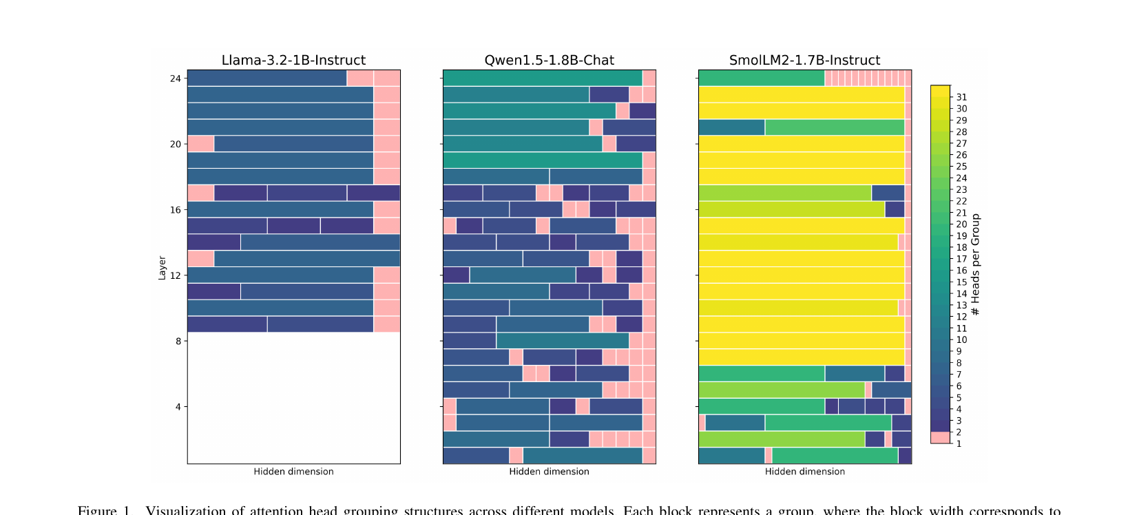
Figure 3 (paper Fig.1): Visualization of attention head grouping structures across different models. Each horizontal block represents one discovered group; block width corresponds to the group’s total hidden dimension, and color encodes the number of heads merged into that group. The contrast is the entire empirical story of this paper in one picture: Qwen1.5-1.8B-Chat (head dimension 128) ends up with 59 singleton groups — the clustering algorithm essentially refuses to merge almost any heads, because at $d_h=128$ the CKA similarity between distinct heads is low. Llama-3.2-1B-Instruct (GQA, only 8 heads) forms just 17 groups total across all layers — there simply aren’t many heads to work with. SmolLM2-1.7B-Instruct (32 heads, $d_h=64$) shows large, confident merges (note the wide yellow/green bands spanning 20+ heads per group) — this is the case where dynamic grouping actually has room to do its job.

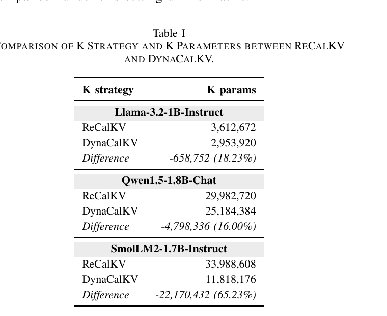
Figure 4 (paper Table I): Key-cache parameter counts, ReCalKV vs. DynaCalKV. The headline numbers: DynaCalKV cuts Key-cache parameters by 18.23% on Llama-3.2-1B-Instruct, a more modest 16.00% on Qwen1.5-1.8B-Chat, and a striking 65.23% on SmolLM2-1.7B-Instruct. Reading this alongside Figure 3 above makes the mechanism obvious: SmolLM2’s large, confidently-merged groups (many redundant heads packed together) are exactly where the greedy rank-adjustment step (Eq. 5) can sacrifice the most redundant rank without much energy loss. Qwen1.5’s near-all-singleton grouping means almost every group is treated individually with little room for the adjustment step to find savings, so the reduction stays modest. Llama’s GQA architecture simply starts with too few heads (8) for either dynamic or fixed grouping to make a dramatic difference — the reduction here is more a side-effect of fewer, larger Key projection layers (16 layers, 512 total dimension) than of clustering quality itself.

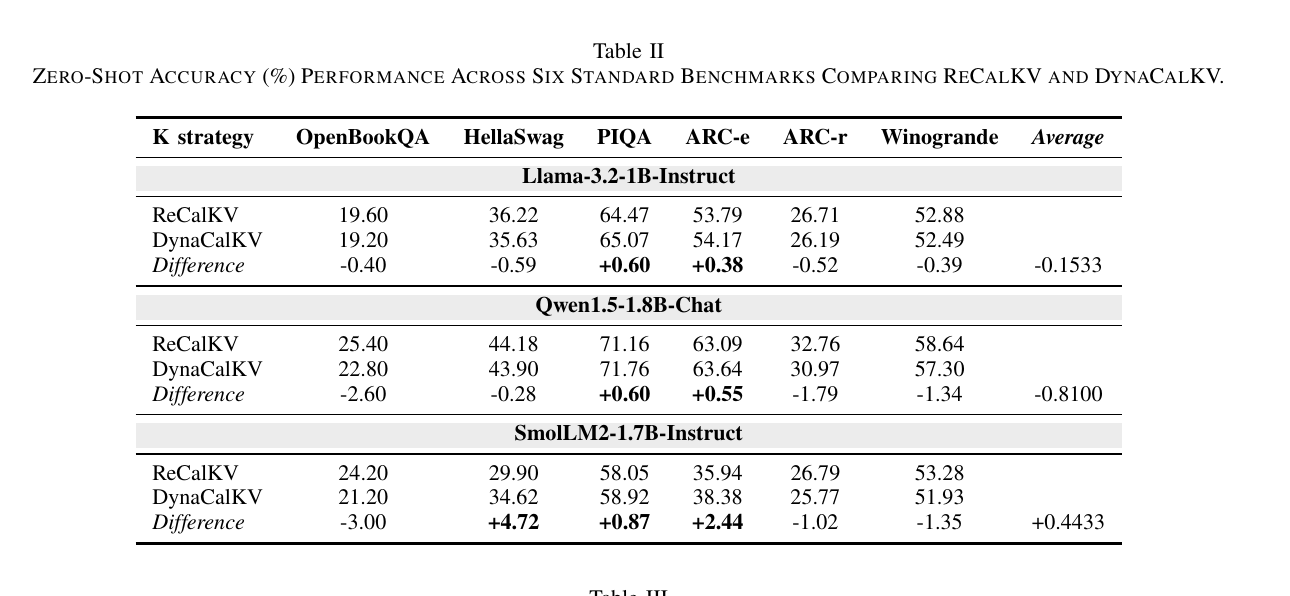
Figure 5 (paper Table II): Zero-shot accuracy across six standard QA benchmarks. This is arguably the most encouraging result in the paper: despite the dramatic parameter reductions above, average accuracy differences vs. ReCalKV are small and mixed in sign — $-0.15$ points on Llama, $-0.81$ on Qwen1.5, and positive $+0.44$ on SmolLM2. Notably, DynaCalKV outperforms ReCalKV on PIQA and ARC-e consistently across all three models (up to $+2.44$ on ARC-e for SmolLM2), suggesting that at least for common-knowledge/factual-retrieval-style tasks, aggressively merging redundant Key heads does not meaningfully hurt — and may even act as a mild regularizer. The picture is less rosy on OpenBookQA and ARC-r (more complex multi-step reasoning), where DynaCalKV consistently loses a small amount of accuracy across all three models, hinting that reasoning-heavy tasks are more sensitive to the fine-grained Key information that aggressive clustering discards.

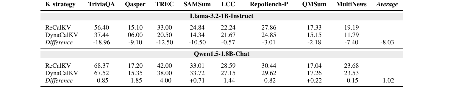
Figure 6 (paper Table III): LongBench long-context evaluation. This table is where the paper’s central cautionary claim becomes concrete and severe. On Qwen1.5-1.8B-Chat (MHA, 16 heads), DynaCalKV is nearly lossless, averaging just $-1.02$ points below ReCalKV, and even improving on SAMSum ($+0.71$) and QMSum ($+0.22$). But on Llama-3.2-1B-Instruct (GQA, 8 heads), the average drop is $-8.03$ points, with catastrophic degradation on retrieval-heavy tasks: $-18.96$ on TriviaQA, $-12.50$ on TREC, $-10.50$ on SAMSum, $-7.40$ on MultiNews. (SmolLM2’s LongBench numbers aren’t reported at all — the paper notes that all three methods, including the ReCalKV baseline, collapse to near-zero performance on that model under LongBench, making any comparison uninformative; this is a real, if awkwardly-timed, gap in the evaluation, discussed further below.) The mechanism the authors propose: GQA models already operate with a minimal, load-bearing set of Key heads (each one non-redundant by construction, since GQA’s whole design point is to avoid keeping redundant heads in the first place); clustering further “merges” already-distinct heads and destroys fine-grained positional/contextual information that long-context retrieval and summarization specifically depend on. Short benchmarks apparently don’t stress this failure mode enough to expose it, which is precisely why the LongBench evaluation — not just the six standard QA benchmarks — was necessary to catch this at all.

Practical takeaway the paper draws (and that I’d endorse): treat DynaCalKV as architecture-aware, not universally beneficial. It is a strong default for standard MHA models with many heads, where it can be applied confidently even in long-context settings. On GQA models with already-thin Key-head counts, it remains usable for short-context tasks but should be applied conservatively — or perhaps skipped in favor of plain ReCalKV — for long-context deployments.

4.1 Interpreting the accuracy/parameter trade-off as a single picture

It is useful to summarize the three-way trade-off (parameter savings, short-context accuracy, long-context accuracy) in one table, since the paper presents these as three separate results but never explicitly juxtaposes them:

Model	Architecture	Key params saved	Zero-shot avg. Δ	LongBench avg. Δ
Llama-3.2-1B-Instruct	GQA, 8 heads	−18.23%	−0.15	−8.03
Qwen1.5-1.8B-Chat	MHA, 16 heads, $d_h{=}128$	−16.00%	−0.81	−1.02
SmolLM2-1.7B-Instruct	MHA, 32 heads, $d_h{=}64$	−65.23%	+0.44	(not reported)

Read this way, the story is stark: the model with the smallest parameter savings (Qwen1.5, 16%) has the safest long-context behavior, while the model with a meaningful but not extreme parameter savings (Llama, 18%) has by far the worst long-context degradation. Parameter savings and quality preservation are not correlated with each other in this table at all — the deciding factor is purely architecture (GQA vs. MHA), which is exactly the paper’s own conclusion, but seeing all three metrics side-by-side makes clear how little the raw compression ratio predicts the outcome. A practitioner scanning only for “how many parameters does this save me” without checking architecture would walk straight into the Llama-style failure mode.

4.2 An additional pattern worth naming: knowledge tasks vs. reasoning tasks

Looking back at Table II (Figure 5), there’s a further pattern worth calling out explicitly, which the paper documents in scattered numbers but never names as a single phenomenon: DynaCalKV consistently gains on common-knowledge/factual-retrieval tasks (PIQA, ARC-e) across all three models, while consistently losing a small amount on tasks requiring multi-step reasoning (OpenBookQA, ARC-r). A plausible explanation is that knowledge/retrieval tasks depend on Key information behaving as a coarse index — you mostly just need to locate roughly the right region of context, and merging redundant heads costs little precision there — while multi-step reasoning may require repeatedly attending back to different fine-grained details across several reasoning steps, details that are exactly what get blurred together when their originating heads get merged. If this explanation holds, it has a direct practical implication: for deployments that are predominantly reasoning-heavy (math, code generation, multi-hop QA), even on a favorable MHA architecture, DynaCalKV’s compression aggressiveness should probably be tuned more conservatively than the paper’s default configuration, rather than assuming the favorable average-case numbers transfer uniformly across task types.

5. Limitations the paper acknowledges

The authors are refreshingly upfront about several constraints, which is worth crediting explicitly:

• Hardware scope. All three models tested are small (1B–2B parameters) and evaluation runs on a single T4 GPU — explicitly attributed to available compute, not a deliberate design choice. Whether the CKA-clustering behavior (and its architecture-dependent failure mode) holds at 7B+ scale, where head counts and dimensions differ substantially, is untested.
• Missing SmolLM2 LongBench numbers. Because ReCalKV, Palu, and DynaCalKV all collapse to near-zero on LongBench for SmolLM2-1.7B-Instruct, the paper simply omits that comparison as “uninformative.” This is honest, but it also means one-third of the long-context evidence for the paper’s flagship MHA case study (SmolLM2 has the most heads and the largest reported parameter savings) is simply absent — we don’t actually know if DynaCalKV holds up in long context for the model where it saves the most parameters.
• Only three models, one calibration set. WikiText-2 is a relatively narrow, English-only calibration corpus; how sensitive the CKA similarity structure and the resulting clusters are to calibration-data choice is not studied.

6. Critical analysis

(a) Weaknesses and flaws specific to this paper. The greedy rank-adjustment heuristic (Section 3.2, Eq. 4–5) is the load-bearing mechanism that determines how much budget gets freed, yet it is a one-shot greedy pass with no optimality guarantee and no comparison against a smarter constrained-optimization baseline (e.g., a proper knapsack DP over discretized rank levels, which would be tractable at this problem scale). Because group sizes under dynamic clustering can vary enormously (from singleton groups to 30+-head groups, per Figure 3), a greedy “cheapest first” heuristic is exactly the kind of allocation problem where locally-optimal choices can compound into a meaningfully suboptimal global allocation. The paper never reports what fraction of the theoretical energy-optimal allocation the greedy heuristic actually achieves, so a reader has no way to judge how much headroom is being left on the table.

Similarly, the choice of $\lambda = 1$ in the cluster-count selection objective (Eq. 6) is justified only by the two terms being “observed to be comparable” — there’s no sensitivity analysis showing how results change as $\lambda$ varies, and no argument for why this should transfer to models with very different energy/rank-utilization scales (e.g., much larger models where a unit of energy loss and a unit of unused rank may not be remotely comparable in magnitude).

(b) Limitations the authors understate or omit. The paper frames its GQA finding (“apply conservatively in long-context settings”) as a nuanced caveat, but the actual number — an 8-point average LongBench drop, with individual tasks losing 10–19 points — is a severe regression, not a minor caveat. For a production system, an 18.96-point drop on TriviaQA is disqualifying, not “conservative use recommended.” The paper’s framing softens what is, functionally, a clear statement that DynaCalKV should simply not be used on GQA models in long-context deployments as currently designed, full stop, pending a fix. Relatedly, the paper never proposes or even sketches a mitigation for the GQA failure mode (e.g., a hybrid rule that falls back to fixed/no grouping specifically for architectures below some head-count threshold) — it diagnoses the problem cleanly but stops short of solving it, despite the fix being conceptually straightforward (detect $h \le$ some threshold, e.g., $h \le 8$, and skip clustering in that regime).

(c) Concrete, specific improvement suggestions. First, add an explicit architecture-aware guard: if the number of Key/Value heads $h$ falls below some threshold (the paper’s own data suggests something like $h \le 8$ is the danger zone), automatically fall back to ReCalKV’s fixed grouping or even no grouping at all, rather than leaving this as a caveat for practitioners to discover themselves. Second, replace the greedy rank-adjustment heuristic with a proper discrete-optimization formulation (even a simple dynamic program over quantized rank levels per group would likely be tractable given the small number of groups per layer) and report how much the greedy version leaves on the table relative to it. Third, run the missing SmolLM2 LongBench evaluation with a different calibration or evaluation protocol that avoids the reported near-zero collapse for all methods, since without it the paper’s strongest parameter-savings result (65.23%) has no accompanying long-context quality evidence at all. Fourth, test on at least one 7B-scale model of each architecture family to establish whether the MHA/GQA dichotomy identified here is a fundamental architectural property or an artifact of the small 1–2B parameter regime studied.

A fifth improvement worth adding: report the linkage criterion used in the agglomerative clustering step (flagged in Section 3.5) and, ideally, an ablation over at least two linkage choices (e.g., average-linkage vs. Ward’s method) to show whether the reported results are sensitive to this specific hyperparameter or robust across reasonable choices. Given that the entire method’s behavior hinges on how heads get clustered, and clustering algorithms are known to be sensitive to linkage choice especially in high-dimensional, noisy similarity spaces (which CKA-derived similarity matrices often are, particularly for larger head dimensions like Qwen1.5’s $d_h=128$), this is not a cosmetic detail — it directly affects whether another team can trust that re-running this method on a new model will reproduce a similar MHA/GQA split in outcomes, or whether the split itself is partly an artifact of one specific clustering configuration.

6.1 A note on evaluation methodology: relative vs. absolute comparisons

One more detail worth surfacing for readers planning to build on this work: the paper’s zero-shot QA evaluation (Table II) and LongBench evaluation (Table III) both compare post-compression accuracy to the ReCalKV baseline, but neither table reports the uncompressed (original, full-precision, no KV-cache compression at all) model’s accuracy on the same benchmarks. This makes it impossible for a reader to judge, from this paper alone, how much total accuracy has been given up relative to an uncompressed model — only how DynaCalKV compares to one specific prior compression method (ReCalKV). If ReCalKV itself already costs, say, 3–4 points of accuracy relative to the uncompressed model on some of these benchmarks (a plausible scenario, given that both methods perform fairly aggressive low-rank compression of the Key cache), then DynaCalKV’s reported "$-0.15$" or "$+0.44$" deltas relative to ReCalKV could still represent a meaningfully larger total gap relative to an uncompressed baseline. This is a common omission across the low-rank KV-cache compression literature more broadly — relative comparisons between compression methods are reported far more often than absolute comparisons to an uncompressed ceiling — but it’s still worth flagging explicitly here, since it directly affects how a reader should interpret the paper’s central “nearly lossless” framing. A reader deciding whether to deploy DynaCalKV in production should independently benchmark the uncompressed model on their own workload before concluding that a small delta relative to ReCalKV also means a small delta relative to no compression at all.

7. Reproducibility notes

• Code/data availability: the paper builds directly on the publicly available Palu repository (arXiv:2407.21118) and re-implements ReCalKV (arXiv:2505.24357) on top of it; no dedicated DynaCalKV repository link is given in the preprint text itself, so reproduction requires re-implementing Algorithm 1 (CKA similarity + agglomerative clustering + energy-based rank init + greedy adjustment) on top of the Palu/ReCalKV codebase.
• Compute requirements: a single NVIDIA T4 GPU is sufficient for all reported experiments (1–2B models), which is a genuinely low bar to reproduce — one of the more practitioner-friendly aspects of this paper.
• Calibration data: WikiText-2, used identically for both the layer-wise Fisher Information budget allocation and the Value-cache calibration refinement (Eq. 8–9).
• Key hyperparameters to match: rank budget $r$ per layer (inherited from Palu’s Fisher-Information-based allocation), candidate cluster-count set $\mathcal{K}$ searched over in Algorithm 1 (not explicitly enumerated in the text — a reproducibility gap), and $\lambda = 1$ in the cluster-selection objective (Eq. 6).
• Evaluation harness: six zero-shot QA benchmarks and eight LongBench datasets, standard and widely available; no custom benchmark construction needed.

7.1 A note on what “architecture-aware” should mean in practice

The paper’s recommendation — “be architecture-aware” — is correct but underspecified as actionable guidance. A practitioner reading this paper and deciding whether to adopt DynaCalKV for their own serving stack needs a concrete decision rule, not just a qualitative caveat. Based on the evidence presented, a reasonable first-pass rule would be: (1) count the number of Key/Value heads $h$ in the target model; (2) if $h \ge 16$ (comfortably inside the “many redundant heads” regime demonstrated by Qwen1.5 and SmolLM2), adopt DynaCalKV with confidence for both short- and long-context workloads; (3) if $h \le 8$ (the GQA regime demonstrated by Llama-3.2-1B), restrict DynaCalKV to short-context workloads only, or skip it entirely in favor of plain ReCalKV for long-context deployments; (4) for the messy middle ground ($8 < h < 16$), this paper simply provides no evidence either way, and a team in that situation would need to run their own LongBench-style validation before trusting either method’s behavior. This kind of explicit decision boundary is easy to derive from the paper’s own numbers, but the paper stops short of stating it this concretely — which is a small but real gap between what the data shows and what the paper’s actionable recommendation says.

8. Conclusion

DynaCalKV is a tightly-scoped, well-executed ablation of a single design decision inside an existing KV-cache compression pipeline: does letting attention-head similarity structure drive dynamic grouping (instead of a fixed group size) improve low-rank Key-cache compression? The answer the paper delivers is genuinely nuanced rather than a blanket “yes”: dynamic grouping recovers substantial additional Key-cache savings (up to 65% fewer parameters) on standard multi-head attention models with many heads, while largely preserving accuracy on both short-context QA and long-context LongBench evaluation — but the same mechanism becomes actively harmful on grouped-query-attention models that already operate with a small, non-redundant set of Key heads, where long-context quality can degrade by double digits. For anyone building or maintaining a KV-cache compression pipeline, the takeaway is less “adopt DynaCalKV” and more “know your architecture before choosing a grouping strategy” — a lesson that likely generalizes to other adaptive-clustering ideas applied to attention heads more broadly, not just to this specific SVD-based compression pipeline.