Libra: Taming Attention Workload Skew in Long-Context LLM Training with Bounded Sequence Pool

Review date: 2026-07-30 Author: Zhongzhu Zhou Paper reviewed: Libra: Taming Attention Workload Skew in Long-Context LLM Training with Bounded Sequence Pool Paper authors: Yan Wang, Xiulong Yuan, Kaiming Yang, Jiaxuan Peng, Pengju Lu, Mingzhen Li, Zhipeng Zhang, Chang Si, Zhixiang Ruan, Hongqing Chen, Linlang Jiang, Siyu Wang, Langshi Chen, Rui Men, Man Yuan, Guangming Tan, Yong Li, Weile Jia, Jingren Zhou arXiv: 2607.23250 Venue/Status: Preprint (cs.DC), July 25, 2026 — University of Chinese Academy of Sciences / Alibaba Group / National University of Singapore

1. Why this paper, and what problem is it actually solving

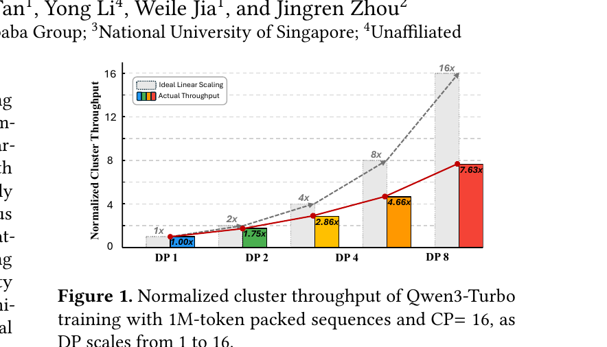
Suppose you are training a long-context LLM at, say, 1M tokens per packed sequence, and someone hands you the following observation: you double your GPU count from 128 to 256 by doubling data parallelism (DP), and your training throughput goes up by… 1.9x, not 2x. You try it again scaling DP from 1 to 16 (16x more GPUs), and you get 4.42x, not 16x. Something is eating roughly three-quarters of your expected scaling. It is not a networking bug, not a bad NCCL version, not GPU flakiness. It is a statistical property of your dataset colliding with how attention cost scales, and it is happening even though every GPU is nominally doing the “same amount of work” by token count.

This is the problem Libra tackles, and it is one of those papers where the diagnosis is at least as valuable as the fix. The authors (from Alibaba’s Qwen training team, with academic collaborators) show that sequence packing — the standard trick for keeping GPU memory and compute uniform across data-parallel replicas — does nothing to balance attention compute, because attention cost scales quadratically with sequence length while packing only balances the linear token count. Their fix, Libra, is now running in production on Qwen-series training jobs from 32K to 1M tokens, across thousands of GPUs, having already accumulated hundreds of thousands of GPU-hours.

If you work anywhere near distributed LLM training — pipeline parallelism, context parallelism, data loading, or cluster scheduling — this paper is worth reading closely for one specific idea that generalizes well beyond attention: when you need to redistribute an imbalanced workload across a scaling cluster, you do not have to make the redistribution domain scale with the cluster. You can hold it fixed, using classical statistics (the law of large numbers) to tell you how big “fixed” needs to be, and add more fixed-size domains as the cluster grows. This is a genuinely reusable systems-design pattern, not just an attention-specific hack.

Prerequisites: what you need to know before diving in

If you are already fluent in DP/PP/CP parallelism, sequence packing, and FlashAttention-style variable-length kernels, skip ahead to Section 2. Otherwise, here is the minimum vocabulary.

Data Parallelism (DP). Split the batch across replicas: each replica holds a full copy of the model and processes a disjoint slice of the global batch, then all replicas synchronize gradients (typically via AllReduce) before the optimizer step. The slowest replica in a DP group stalls everyone else — this “straggler” effect is central to this paper.

Pipeline Parallelism (PP). Split the model’s layers across stages, feeding microbatches through them like an assembly line (GPipe-style). If different microbatches take very different amounts of time to process, the pipeline develops “bubbles” — idle gaps where later stages wait for a slow earlier stage to finish an unusually heavy microbatch.

Context Parallelism (CP). For very long sequences, even a single sequence’s activations and attention computation do not fit comfortably on one GPU. CP splits a single sequence’s core-attention computation across a group of workers — either along the sequence axis (Ring Attention, which circulates KV blocks around a ring) or along the head axis (DeepSpeed Ulysses, which exchanges Q/K/V tensors so each worker computes full attention for a subset of heads). This paper treats CP as an abstraction for “the workers that jointly compute one packed sequence’s core attention,” which subsumes tensor parallelism on the attention path.

Sequence packing. Real training corpora contain samples of wildly different lengths (a chat turn might be 200 tokens; a code repository dump might be 60K tokens). Padding every sample up to the longest one in a batch wastes enormous compute. Instead, packing concatenates multiple short samples into one fixed-length “packed sequence” of length $L$ (e.g., 256K or 1M tokens), separated by a block-diagonal causal mask so no sample can attend across another sample’s boundary. This keeps every packed sequence the same token count $L$, which balances memory and any linear-cost operator (MLPs, layernorms) uniformly across replicas.

Why packing does not balance attention. Multi-head self-attention has a cheap linear part (Q/K/V/output projections, cost $O(l)$ in sequence length $l$) and an expensive quadratic part (core attention itself, cost $O(l^2)$, dominant at long context). For a packed sequence containing samples of length $\{\ell_j\}$, the total attention FLOPs scale as $\sum_j \ell_j^2$ — the sum of squares, not the sum. This is the crux of the whole paper: two packed sequences with identical total token count $L$ can have very different $\sum_j \ell_j^2$ if one packs “one 40K-token sample + short filler” and the other packs “ten 4K-token samples.” The first does roughly 10x the attention FLOPs of the second despite occupying exactly the same memory footprint. Equal token counts silently conceal unequal attention workloads.

FlashAttention / variable-length attention kernels. Modern attention implementations (FlashAttention and its variable-length variants) fuse the QK^T, softmax, and weighted-sum-with-V steps into a single memory-efficient kernel that never materializes the full $l \times l$ attention matrix. This is what makes it feasible to run attention over ragged, packed, multi-sample sequences at all — the paper builds directly on an unmodified variable-length FlashAttention kernel and never touches its internals.

Law of Large Numbers (LLN), briefly. If you sum up $n$ independent, identically-distributed random variables with finite variance, the relative spread of that sum (its coefficient of variation, or standard deviation divided by mean) shrinks like $1/\sqrt{n}$. In other words: averaging over more independent things concentrates the average closer to the true mean. This is the single statistical fact that Libra’s entire design is built around — it says that if you group enough packed sequences together into one workload-redistribution pool, the pool’s total attention workload will concentrate near the dataset’s mean workload, even though any individual sequence in that pool might be wildly larger or smaller than average.

With this vocabulary, the rest of the paper reads cleanly.

2. Architecture overview: what Libra actually builds

Libra is a drop-in context-parallel attention operator plus a pluggable data sampler — it requires zero changes to model layers, optimizers, gradient accumulation, checkpointing, or the pipeline schedule. You swap in libra_attention in place of your existing CP core-attention call, and it handles workload redistribution invisibly underneath.

flowchart TD
    A["Global batch of GBS packed sequences arrives"] --> B["VRSP: CPU-side heavy-light\nreordering into fixed-size P-sequence pools"]
    B --> C["Each DP replica loads its assigned\npacked sequence for this GA index"]
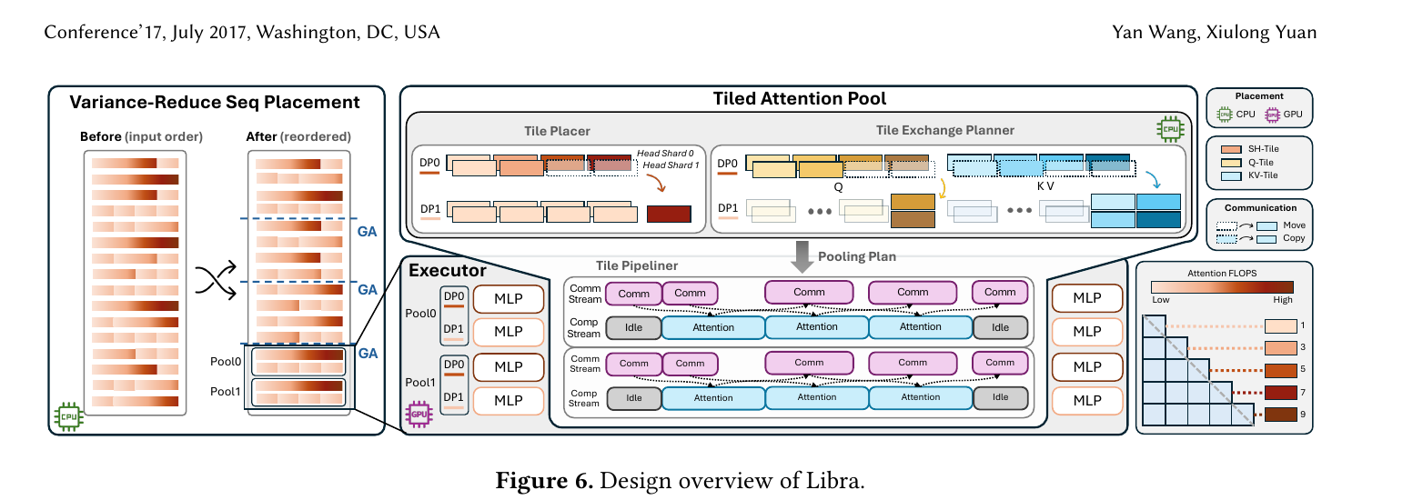
    C --> D["TAP Tile Placer: split each sequence\ninto Sequence x Head SH-Tiles,\nestimate FLOPs, assign across pool's W workers"]
    D --> E["Tile Exchange Planner: dedupe KV fetches,\nbuild per-worker transfer schedule"]
    E --> F["TAP Pipeliner: chunk transfers by head axis,\noverlap dispatch/return with FlashAttention compute"]
    F --> G["Unmodified FlashAttention kernel\nruns each SH-Tile's attention"]
    G --> H["Outputs returned to Q-home workers,\nfeed into unchanged MLP/optimizer path"]

Figure 1 (self-drawn, Mermaid): Libra’s end-to-end pipeline, from the global batch down to the unmodified attention kernel. Everything left of the FlashAttention call is Libra; everything to its right (MLP, optimizer, checkpointing) is untouched.

Libra attacks the imbalance problem at two levels, using three components:

1. Variance-Reduced Sequence Placement (VRSP) — balances aggregate attention workload across sequence pools, by cleverly assigning which packed sequences land in which pool.
2. Tiled Attention Pooling (TAP) — balances workload within a pool, by decomposing each packed sequence into fine-grained sequence-by-head tiles and spreading them across the pool’s workers.
3. TAP Pipeliner — overlaps the tensor movement that TAP’s rebalancing introduces with the actual attention computation, so the load-balancing “costs” as little wall-clock time as possible.

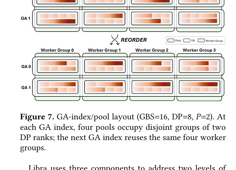
The central abstraction tying all three together is the sequence pool: a fixed-size group of $P$ DP replicas (and their CP groups), defined at a given pipeline stage and gradient-accumulation (GA) index. Crucially — and this is the paper’s core design decision — $P$ stays fixed as the cluster’s DP degree grows. Scaling DP from 8 to 16 does not make each pool twice as large; it creates twice as many fixed-size pools running side by side. This is the “bounded sequence pool” of the title, and it is where the law of large numbers earns its keep.

Data flow at a glance

flowchart LR
    subgraph DataPath["Data path (CPU, offline)"]
        Meta["Sequence-length metadata\nfor GBS packed sequences"]
        VRSP["VRSP: heavy-light greedy\nplacement into K pools"]
        Meta --> VRSP
    end
    subgraph PoolExec["Per-pool execution (each GA index)"]
        TilePlan["CPU Tile Placer + Tile\nExchange Planner (per iteration)"]
        Exec["GPU executor: fetch tiles,\nrun FlashAttention, return outputs"]
        TilePlan --> Exec
    end
    VRSP -->|"reordered sequence -> pool assignment"| PoolExec

Figure 2 (self-drawn, Mermaid): Two clearly separated planning domains — VRSP operates once per optimizer step across the whole GBS window, while TAP’s tile placement operates once per training iteration within each pool. Both run on CPU, ahead of and alongside the GPU critical path, so no placement decision blocks GPU execution.

Here is Libra’s actual architecture diagram from the paper, showing how VRSP feeds into the Tiled Attention Pool’s Tile Placer, Tile Exchange Planner, and pipelined Executor:

And here is the GA-index/pool layout concretely, showing how pool membership stays fixed across gradient-accumulation indices while different (reordered) sequences flow through those fixed worker groups:

The rest of this review works through each component’s math and design rationale in order: why fixed-size pools work at all (Section 3), how VRSP fills them well despite the finite-window / long-tail problem (Section 4), how TAP balances work inside a pool (Section 5), how the Pipeliner hides the resulting communication (Section 6), and then the experimental evidence (Section 7) and a critical assessment (Section 8).

3. Why bounded pools work: the law of large numbers, derived

3.1 The workload proxy and why equal tokens do not mean equal FLOPs

For a packed sequence $S$ containing raw samples with lengths $\{\ell_j\}$, the paper defines an attention-workload proxy:

$$w(S) \propto \sum_j \ell_j^2 \tag{1}$$

This absorbs constants (causal factor, number of heads, head dimension) into the proportionality constant, since those are fixed across all packed sequences and do not affect relative comparisons. The intuition: attention cost is quadratic in each individual sample’s length (because attention computes pairwise interactions within a sample, blocked by the causal mask at sample boundaries), so a packed sequence’s total attention cost is the sum of its constituent samples’ squared lengths, not the square of the total length. This is why one 40K-token sample contributes roughly 10x the attention FLOPs of ten 4K-token samples: $40000^2 = 1.6\times10^9$ versus $10 \times 4000^2 = 1.6\times10^8$ — a 10x gap, despite both packings summing to 40K tokens.

Production long-context corpora are strongly long-tailed: the paper’s 1M-token dataset has a median raw-sample length of only 644 tokens, but a p99 of 71,006 tokens. Because of the quadratic proxy, this length skew becomes a much larger skew in attention workload — a handful of packed sequences that happen to contain long tail samples will dominate attention FLOPs, while most packed sequences (built mostly from short samples) are comparatively cheap.

3.2 Deriving the concentration bound for a fixed-size pool

Here is the derivation the paper sketches, filled in step by step. Let $X = w(S)$ be the workload of one packed sequence, with population mean $\mu$, standard deviation $\sigma$, and coefficient of variation $CV = \sigma/\mu$. Within one optimizer-step window (one global-batch-size, $GBS = D$ packed sequences), group them into pools of size $P$, giving $K = D/P$ pools. Let $L_k$ be pool $k$‘s aggregate workload — i.e., the sum of the $w(S)$ values of the $P$ sequences assigned to it.

Step 1 — apply the Central Limit Theorem (CLT) to each pool’s sum. Under the analytical approximation that packed-sequence workloads are grouped randomly and are approximately independent and identically distributed (IID) with finite variance, the CLT tells us each pool’s sum $L_k$ is approximately Gaussian:

$$L_k \;\approx\; \mathcal{N}\!\left(P\mu,\; P\sigma^2\right) \tag{2}$$

The mean scales linearly with $P$ (adding $P$ independent things adds their means), and the variance also scales linearly with $P$ (adding $P$ independent things adds their variances) — so the standard deviation scales as $\sqrt{P}\sigma$, not $P\sigma$.

Step 2 — normalize to get the imbalance ratio. Define the cluster-wide maximum normalized load $R = \max_k L_k / (P\mu)$; perfect balance is $R=1$. Dividing $L_k$ by its mean $P\mu$ gives a normalized quantity with mean 1 and standard deviation

$$\frac{\sqrt{P}\sigma}{P\mu} = \frac{\sigma/\mu}{\sqrt{P}} = \frac{CV}{\sqrt{P}}. \tag{3}$$

This is the key step: the relative spread of one pool’s normalized load shrinks as $1/\sqrt{P}$ — exactly the law of large numbers in action. Bigger pools concentrate more tightly around the mean, in relative terms.

Step 3 — account for taking a maximum over $K$ pools. But we don’t just care about one pool’s spread — we care about the worst pool in the whole cluster, since that is the one that becomes the DP/PP straggler. For $K$ approximately-Gaussian, approximately-independent normalized sums, a standard extreme-value approximation for the expected maximum of $K$ standard Gaussians is $\sqrt{2\ln K}$. Combining this with the per-pool spread from Step 2:

$$E[R] \;\approx\; 1 + \frac{CV}{\sqrt{P}}\sqrt{2\ln K} = 1 + \frac{CV}{\sqrt{P}}\sqrt{2\ln(D/P)}. \tag{4}$$

The paper is careful to flag this as an analytical approximation, not a claim that production packed-sequence workloads are strictly IID — real corpora have correlations (e.g., data loaders often shuffle within limited windows, and packing itself creates dependencies between which samples end up together).

Interpreting Equation 4. As $P$ grows, the $CV/\sqrt{P}$ factor shrinks — larger pools concentrate more tightly, which is the good news. But $K = D/P$ shrinks as $P$ grows (fewer, bigger pools for a fixed $GBS = D$), and $\sqrt{2\ln K}$ grows slowly with $K$ — so having more, smaller pools makes the maximum-over-pools term worse only logarithmically. Practically, this means: bare LLN concentration alone converges too slowly at the moderate pool sizes ($P \le 16$) that communication efficiency demands. Figure 4 in the paper (residual inter-pool imbalance vs. pool size) shows exactly this: at $P=8$, random grouping still leaves $R-1 \approx 1.08$ on the 256K dataset and $\approx 0.90$ on the 1M dataset — a worst pool with more than double the mean workload. Even at $P=64$ — already too large to keep communication cheap — the residual is still 0.09 and 0.08. This is the paper’s motivation for not relying on random placement, which brings us to VRSP.

3.3 The scaling principle this derivation licenses

The payoff of this whole derivation is a specific, falsifiable claim: the pool size $P$ required for a target concentration level is governed by the workload distribution’s $CV$ and the desired imbalance level — not by the DP degree. Once you have picked a $P$ that gives acceptable concentration for your corpus, you do not need to grow $P$ as DP scales out. You just add more pools of that same fixed size. This is why Libra’s pools remain fixed at $P \le 16$ (in practice $P=8$ for both evaluated workloads) even as DP scales from 1 to 16 across the paper’s experiments, and it is the mechanism by which the scope of every attention-workload redistribution — and therefore its communication domain — stays bounded regardless of cluster size.

Design-choice discussion: why not scale the pool with the cluster (DistCA’s approach)? The obvious alternative is what DistCA does: disaggregate core attention across the entire cluster’s worker pool ($P = DP$), maximizing the workload-aggregation scope. The paper’s own analysis of Equation 4 explains why this is a double-edged trade: a larger pool does concentrate aggregate workload better (bigger $P$, smaller $CV/\sqrt{P}$), but it also (a) grows the communication domain proportionally, potentially crossing low-bandwidth inter-supernode links, and (b) exposes the scheduling to more independent sources of device-runtime variance — a placement that is balanced in estimated FLOPs is not necessarily balanced in wall-clock time, because more workers means more chances for one of them to be transiently slow. The paper backs this second point with a direct measurement: running the same 32K causal-attention input on 256 identical GPUs for 500 steps, discarding the fastest/slowest outlier each step, the per-step (slowest − fastest)/fastest spread averages 7.01% and reaches 15.07% — pure hardware-runtime variance with zero data-workload imbalance. A cluster-wide pool inherits all of this noise into its balancing decisions; a small, fixed pool is exposed to far less of it. This is a legitimate boundary condition worth flagging: Libra’s approach trades some theoretically-achievable balance (a bigger pool could in principle balance FLOPs more tightly) for materially lower communication and runtime-variance exposure — and the paper’s own numbers suggest this trade is worth making at practical scales, but it is a trade, not a free lunch.

4. Variance-Reduced Sequence Placement (VRSP): filling pools well, not randomly

Section 3 established that bare random grouping into fixed-size pools leaves too much residual imbalance at practical $P$. VRSP is the mechanism that closes this gap — not by making the pools bigger, but by choosing which packed sequences go into which pool more cleverly, using all the placement freedom available within one optimizer-step window.

4.1 What VRSP is allowed to touch, and what it must preserve

VRSP’s scheduling unit is a complete packed sequence — it never splits a packed sequence or changes its internal packing (which raw samples share a packed sequence). Given $GBS = D$ packed sequences in one optimizer-step window and target pool size $P$, VRSP forms $K = D/P$ pool instances, each receiving exactly $P$ packed sequences, using the workload proxy from Equation 1:

$$F_i = w(S_i) \propto \sum_j \ell_{ij}^2 \tag{5}$$

It may reorder packed sequences across GA indices, DP replicas, and pools — but it preserves the raw-sample multiset of the entire optimizer step. This constraint matters a great deal and is worth dwelling on: it means VRSP cannot change which raw training samples contribute to a given optimizer update, only how those samples are spatially arranged across workers. This is what the paper calls the “step-equivalence requirement,” and it is the property that distinguishes VRSP from competing approaches like WLB-LLM’s outlier-deferral mechanism, which pushes an unusually large sample into a later optimizer step — changing that step’s sample multiset and, in the authors’ view, changing training semantics in a way they are unwilling to accept.

4.2 The algorithm: exact-cardinality greedy placement (constrained LPT)

VRSP adapts the classic Longest-Processing-Time-first (LPT) scheduling heuristic — originally designed for balancing job loads across machines — with one added constraint: every pool must receive exactly $P$ sequences, no more, no fewer (an “exact-cardinality” constraint that classical LPT does not need to satisfy, since classical LPT only cares about balancing load, not enforcing equal group sizes).

Here is the algorithm, unpacked step by step:

Algorithm 1: Variance-Reduced Sequence Placement

Input:  packed sequences {S_i} for i = 0 .. GBS-1;  pool size P
Output: reordered sequence list S'

1.  for each S_i: compute F_i = sum_j (length of raw sample j in S_i)^2
2.  K = GBS / P                      # number of pools
3.  initialize K empty pools
4.  order = sort sequences by DECREASING F_i, breaking ties by increasing index i
5.  H = min-heap of (current_load[k], pool_id k) over all NON-FULL pools
6.  for each sequence S_i in `order`:
7.      (load_k, k) = pop the minimum-load entry from H
8.      assign S_i to pool k;  load_k += F_i
9.      if pool k now has fewer than P sequences:
10.         push (load_k, k) back onto H
11.         # (if pool k is now full, it is simply NOT pushed back —
12.         #  this enforces the exact-cardinality constraint)
13. S' = concatenate all pools' sequences in GA-major, pool-minor order
14. return S'

Why heaviest-first ordering matters (the intuition). Process the heaviest (most attention-expensive) packed sequences first, while every pool is still empty and available as a destination. Each heavy sequence goes to whichever pool currently has the least accumulated load — this is the standard greedy LPT move, and it is provably good for classical (non-cardinality-constrained) load balancing because it prevents any single pool from silently accumulating multiple heavy sequences early, before the algorithm “notices.” Then, as the algorithm works down to progressively lighter sequences, it uses them to fill in the residual gaps between pools — the lighter sequences are exactly the flexible material needed to top off whichever pools are still slightly under target. If you instead processed sequences in a random or lightest-first order, a late-arriving heavy sequence could be forced into whichever pool happens to have room left, regardless of how loaded that pool already is — precisely the failure mode VRSP is designed to avoid.

Why the exact-cardinality constraint needs special handling. The min-heap in the algorithm only contains non-full pools (line 5/9-10) — once a pool has received its quota of $P$ sequences, it is permanently removed from consideration, even if its current load happens to still be below other pools’ loads. This is necessary because the whole point is to keep every pool at exactly $P$ sequences (so that pool sizes, and therefore worker-group sizes, are uniform and predictable); without the exact-cardinality constraint, ordinary LPT would happily keep piling sequences onto whichever pool is lightest, producing pools of very different sizes even if their loads end up balanced — which would break the fixed $W = P \cdot CP$ worker-group abstraction that the rest of Libra (VRSP’s pool boundaries, TAP’s worker assignment) depends on.

Complexity. Writing $D = GBS$, the procedure sorts the $D$ sequences ($O(D \log D)$) and performs one heap push/pop per sequence over at most $K$ live pool entries ($O(D \log K)$), for a total of $O(D \log D + D \log K) = O(D \log D)$ time and $O(K)$ pool-state space. This runs entirely on CPU at data-loading time, off the GPU critical path, and touches neither the TAP tile-placement logic nor the model’s execution path — it only changes the order in which packed sequences are handed to DP replicas.

A candid caveat the paper states explicitly: this is a practical exact-cardinality heuristic, and the authors do not claim it inherits classical LPT’s worst-case approximation guarantee (the textbook bound that LPT is within 4/3 of optimal for makespan scheduling) once the exact-cardinality constraint is added. That guarantee was proven for unconstrained LPT; adding the “every bin gets exactly $P$ items” constraint changes the combinatorial structure of the problem, and the paper does not re-derive a bound for the constrained variant. What backs VRSP’s effectiveness is empirical measurement, not a re-proven worst-case theorem — a limitation worth being explicit about even though the empirical results (below) are strong.

4.3 Does it actually work? The empirical concentration numbers

Figure 8 in the paper (not reproduced here, but the core numbers are worth quoting directly) sweeps VRSP against three baselines — Random grouping, Zigzag ordering, and Zigzag+Swap — across pool sizes $P \in \{2,4,8,16,32,64\}$ on both the 256K and 1M datasets at $GBS=128$. The result: at $P=8$, VRSP drives the residual inter-pool imbalance $R-1$ down to 0.0050 on 256K and 0.0066 on 1M — compared with 1.077 and 0.525 respectively under naive random grouping (i.e., roughly a 150-200x reduction in residual imbalance at the same pool size). VRSP also consistently and substantially outperforms both Zigzag and Zigzag+Swap at every evaluated pool size on both datasets. The gap is not subtle: production-sampler-order grouping would need a dramatically larger pool (well beyond what communication bandwidth allows) to reach the same level of balance that VRSP achieves at $P=8$. Table 1 in the paper additionally shows this holds stably across different global batch sizes ($GBS \in \{32, 64, 128, 256\}$): doubling $GBS$ leaves the $P=8$ VRSP-corrected imbalance essentially unchanged, while the uncorrected production-order imbalance would require an even larger pool to compensate as $GBS$ grows. This is exactly the practical payoff of the LLN-guided design: pool size is decoupled from both DP scale and batch-size scale.

5. Tiled Attention Pooling (TAP): balancing work inside a pool

Even after VRSP balances the aggregate workload assigned to each pool, the $W = P \cdot CP$ individual workers inside one pool can still be imbalanced relative to each other — VRSP operates at the granularity of whole packed sequences, but a single packed sequence’s attention work is not automatically spread evenly across the CP group processing it. TAP is the mechanism for this finer-grained, intra-pool rebalancing.

5.1 SH-Tiles: the atomic unit of rebalancing

TAP decomposes each packed sequence’s attention computation along two axes simultaneously: the sequence axis and the head axis.

• Sequence axis: each packed sequence is cut at global token positions into blocks of at most $B$ tokens (a configurable block size). Crucially, TAP does not add extra cuts at raw-sample boundaries — a block can freely straddle multiple samples, and the final block of a sequence may be shorter than $B$. This keeps the tiling scheme decoupled from the packing scheme.
• Head axis: the $h_q$ query heads are split into $H$ equal-width shards, where $H$ divides $h_q$ evenly. $H$ is a single fixed configuration value shared across every pool, layer, and packed sequence in one training run — it is not re-tuned per-tile.

The combination gives the SH-Tile (Sequence-Head Tile):

$$\text{SH-Tile } t = (\text{sequence\_block } b,\ \text{head\_shard } h) \tag{6}$$

This is the smallest independently-placeable core-attention task in Libra — the placer’s job is to assign every SH-Tile in a pool to one of the pool’s $W$ workers so that each worker ends up with roughly equal estimated FLOPs.

Why not just split along the sequence axis (the more conventional choice)? This is the paper’s most interesting design-choice discussion, because the “obvious” alternative — splitting purely along the sequence axis (as Ring Attention and its relatives do) — turns out to have a real flaw for load balancing specifically (as opposed to raw compute distribution, where it’s a fine well-established choice). The argument has two parts:

1. Uniformity of compute and communication. Equal head-axis chunks have identical query-key interaction patterns, identical Q/K/V/output byte volumes, and identical execution structure — every head shard does “the same shape of work.” Sequence-axis chunks do not have this property: under a causal mask, later sequence blocks in the causal order are inherently more expensive (a later query token attends to a longer prefix of keys) than earlier blocks of the same token-length, so fixed-token sequence chunks are not FLOPs-uniform. You could instead build fixed-FLOPs sequence chunks, but then different chunks contain different numbers of query tokens, so their Q/K/V/output communication volumes differ — you gain compute uniformity but lose communication uniformity. Among the sequence and head axes considered in this work, only the head axis provides both properties simultaneously.
2. Kernel-efficiency sensitivity. The paper directly measures FlashAttention throughput as a function of per-call sequence-block length and head count (their Figure 5). The result: normalized FlashAttention throughput is comparatively insensitive to reducing the number of heads per call, but shortening the sequence-block length degrades kernel efficiency much faster. In other words, splitting along heads costs you comparatively little raw kernel efficiency, whereas aggressively shortening sequence blocks (to get finer-grained scheduling units) actively hurts the underlying FlashAttention kernel’s throughput.

Where head-axis splitting has a boundary condition. The paper is explicit that this analysis is scoped to “the sequence and head axes considered in this work” for dense causal self-attention — it does not claim this ordering holds for sparse or linear attention variants, which the paper explicitly places out of scope (“balancing sparse or linear attention variants is left to future work”). It’s also worth noting head-splitting has a hard ceiling: $H$ can only be increased up to $h_q$ (you cannot split more finely than one query head per shard), and Section 5.4 below shows there is a subtler ceiling tied to the number of KV heads too.

5.2 KV groups and why cross-sample tiles do not need extra masking logic

A KV group is defined as $g = (j, h)$: the complete K/V tensors of raw sample $j$ on head shard $h$. Multiple query blocks belonging to the same sample and head shard can share one KV group — this is pure reuse bookkeeping, since fetching K/V once and reusing it for several query blocks is strictly cheaper than re-fetching per query block.

Even when a query block only needs a causal prefix of a sample’s keys (because of the causal mask), the runtime still fetches the complete KV group for that sample and applies the causal mask during attention computation — it does not try to fetch a masked subset. This is a deliberate simplicity trade-off: fetching exactly the causally-required prefix would save some bytes for early blocks, but would complicate the deduplication logic (Section 6.1) that lets multiple destinations share one fetch of a KV group. A cross-sample SH-Tile (one whose sequence block straddles multiple raw samples) therefore references the set of KV groups for every sample it intersects:

$$K(t) = \{(j,h) \mid j \text{ intersects tile } t = (b,h)\} \tag{7}$$

5.3 FLOPs estimation for a tile

Each SH-Tile’s estimated attention FLOPs must correctly account for the causal mask and for cross-sample fragments, without charging “padding” for the parts of a block that a query does not actually attend to. The paper’s estimate, for a block $b$ covering sample-local query positions $a_{bj}, \ldots, e_{bj}-1$ in every intersected raw sample $j$:

$$f_{b,h} \propto \frac{h_q}{H} \sum_{j:\, b \cap j \neq \emptyset} \ \sum_{q=a_{bj}}^{e_{bj}-1} (q+1) \tag{8}$$

Unpacking this formula. The inner sum $\sum_{q=a_{bj}}^{e_{bj}-1}(q+1)$ counts the actual number of causal query-key pairs for sample $j$‘s portion of this block: query position $q$ (0-indexed, sample-local) attends causally to positions $0, \ldots, q$, which is $q+1$ keys. Summing this over the block’s query range within sample $j$ gives the true triangular count of causal interactions for that fragment — not $B^2$ or any padded approximation. The outer sum over $j$ accumulates this across every sample the block straddles (handling cross-sample blocks correctly), and the $h_q/H$ factor scales by the number of query heads in this shard. Because this estimate depends only on sequence-length metadata and the fixed tile configuration $(B, H)$ — not on the actual K/V tensor values — it can be computed cheaply and deterministically on CPU, ahead of time, with no online profiling required, and the resulting assignment can be reused across every Transformer layer that shares the same layout (since every layer has the same sequence lengths and mask structure, only the actual Q/K/V tensor values differ layer to layer).

5.4 Communication-aware SH-Tile placement

Once every tile’s estimated FLOPs $f_t$ is known, TAP needs to decide which worker executes each tile — and this decision should account for the fact that moving a tile to a non-local worker costs communication (transferring Q, K/V, and the returned output).

Each tile $t$ has one Q-home worker $q(t)$ that supplies its Q tensor and receives its output. If a tile is placed on a different worker than its Q-home, both the Q tensor and the returned output must be transferred; if it’s placed on its Q-home, neither transfer is needed. Separately, if the destination worker already holds (from a previous tile placement) one of the KV groups a tile references, that KV group’s transfer can be skipped too. This gives the incremental communication cost of placing tile $t$ at destination $r$:

$$\Delta_{\text{comm}}(t, r) = \sum_{g \in K(t) \setminus C_r} V_g \;+\; \mathbb{1}[r \neq q(t)]\left(V_Q(t) + V_O(t)\right) \tag{9}$$

where $V_g$, $V_Q(t)$, $V_O(t)$ are the byte volumes of KV group $g$, tile $t$‘s Q tensor, and tile $t$‘s output, respectively, and $C_r$ is the set of KV groups destination $r$ has already committed to fetch. The first term charges for any KV groups not already resident at $r$; the second term (via the indicator function $\mathbb{1}[\cdot]$) charges the Q/output transfer cost only if $r$ is not the tile’s Q-home.

Algorithm 2: Communication-Aware SH-Tile Placement

Input:  tiles T; workers W; slack tau = 0.03
Output: assignment sigma (tile -> worker)

1. C = (1 + tau) * (sum of f_t over all tiles) / |W|   # soft per-worker load target
2. order = sort tiles by DECREASING f_t, then tile ID
3. for each tile t in order:
4.     F = { r in W : current_load[r] + f_t <= C }      # workers with headroom
5.     if F is not empty:
6.         r* = argmin over r in F of (delta_comm(t, r), current_load[r], r)
7.     else:
8.         r* = argmin over r in W of (current_load[r], delta_comm(t, r), r)  # fallback
9.     sigma(t) = r*;  current_load[r*] += f_t
10.    C_{r*} = C_{r*} union K(t)                        # remember newly-resident KV groups
11. return sigma

Reading the algorithm. It is a load-target-guided, communication-aware greedy placer: first, it computes a soft per-worker load target $C$ that’s $(1+\tau)$ times the perfectly-even share, with $\tau=0.03$ fixed across all configurations (a 3% slack). It then processes tiles heaviest-first (same LPT-style intuition as VRSP: place the hardest-to-fit items while all destinations still have room). For each tile, it restricts attention to workers that would stay under the soft target $C$ if this tile were added, and among those, picks the one minimizing incremental communication (breaking ties by current load, then worker ID for determinism). If no worker has enough headroom (line 7-8), it falls back to picking the globally least-loaded worker, prioritizing balance over communication in that edge case.

Design-choice discussion: why prioritize load-target compliance over pure communication minimization? The alternative would be to always pick the worker minimizing $\Delta_{\text{comm}}$, letting load balance emerge as a side effect. The paper’s ordering — filter by load headroom first, minimize communication second — reflects a considered priority: an unbalanced pool directly costs wall-clock time (the slowest worker sets the pool’s execution time), while suboptimal communication placement costs comparatively less (much of it gets hidden by the Pipeliner in Section 6). The paper is candid about the resulting boundary condition: $C$ guides the trade-off, it does not provide a worst-case load guarantee. In particular, a single tile can be individually larger than the remaining headroom of every worker — no soft target can prevent an indivisible large tile from overshooting some worker’s target once placed. This is structurally similar to the “indivisible outlier” problem VRSP faces at the sequence level, just recurring one level down at the tile level; the paper does not offer a further fix (like splitting an oversized tile) for this residual case.

6. The TAP Pipeliner: hiding the communication TAP introduces

Rebalancing SH-Tiles across workers is only a net win if the resulting Q/KV/output transfers don’t simply eat back the time saved by better load balance. The TAP Pipeliner’s job is to overlap this tensor movement with the attention computation itself.

6.1 Deduplication of KV transfers

Before even discussing overlap, one important efficiency detail: KV transfer is deduplicated per sample, head shard, and destination worker. If multiple SH-Tiles at the same destination reference the same KV group, that group is fetched exactly once for that destination and reused for every referencing tile — two different destinations, however, do fetch separate copies (there is no cross-worker KV caching in this scheme). Local Q/output paths (tile stays on its Q-home) and already-resident KV groups require no transfer at all. This deduplication is what makes the load-target-aware placement in Algorithm 2 meaningfully cheaper than a naive “fetch everything independently per tile” scheme would be.

6.2 Equal-head chunk construction: the trick that makes pipelining possible

Here is the key insight that makes overlap effective: every SH-Tile assigned to a worker has the same head-shard width, $h_q/H$. The executor first concatenates all of a worker’s assigned SH-Tiles along the sequence/variable-length-batch dimension, producing one aggregate workload with head-width $h_q/H$. It then splits this aggregate workload’s head dimension into $M$ equal pieces (with $M$ dividing $h_q/H$ evenly; the paper fixes $M=4$ in all experiments). Chunk $m$ then contains the $m$-th head-piece of every SH-Tile assigned to this worker.

Why this matters: even though the worker’s assigned SH-Tiles can have wildly heterogeneous sequence-block lengths (some tiles cover long sequence blocks, others short ones, per TAP’s balancing decision), every chunk contains the same proportional fraction of every tile. This means every chunk has the same estimated FLOPs, the same Q/output byte volume, the same KV byte volume, and the same execution structure as every other chunk for that worker — chunks are pipeline-uniform by construction, which is exactly what you need for predictable, evenly-spaced overlap.

6.3 Asynchronous overlap schedule

The runtime issues non-blocking communication and delays synchronization until the transferred tensors are actually consumed by compute. Concretely:

Dispatch chunk 0's Q/K/V  (non-blocking)
for m = 0 to M-1:
    wait only for chunk m's input handle (if not already arrived)
    while computing chunk m's attention:
        concurrently dispatch chunk (m+1)'s Q/K/V   [if m+1 < M]
        concurrently return chunk (m-1)'s output     [if m-1 >= 0]
wait for chunk (M-1)'s output-return handle before assembling final output

The runtime waits for an input handle only immediately before computing the corresponding chunk, and waits for outstanding return handles only immediately before assembling the final output. This means chunk 0’s initial dispatch and chunk $M-1$‘s final return are the only two communication events that cannot be hidden — every transfer in between overlaps with some chunk’s attention computation. When each chunk’s attention compute time is at least as long as the concurrent transfer time, up to $(M-1)/M$ of the total communication volume can be hidden behind compute (for $M=4$, up to 75% in the ideal case).

Design-choice discussion: why fix $M=4$ rather than tuning it per-configuration? A larger $M$ gives finer-grained overlap (more, smaller chunks to interleave), theoretically hiding a larger fraction of communication ($(M-1)/M \to 1$ as $M$ grows). But finer chunking also means each chunk’s compute is shorter, making it more likely the compute time no longer covers the transfer time for that chunk (breaking the assumption that overlap fully hides communication), and it adds more kernel-launch and synchronization overhead per chunk. The paper does not present a sweep over $M$, so this specific choice of $M=4$ reads as an engineering default validated by the end-to-end numbers rather than a value derived from first principles — a minor reproducibility gap worth flagging (see Section 9).

Boundary condition, stated directly by the authors: overlap cannot fully hide communication once the pool grows. Their own pool-size sweep (Figure 14, discussed in Section 7.4 below) shows that at larger pool sizes, the unhidden communication leftover keeps growing even though per-worker computation stays balanced — overlap mitigates but does not eliminate the cost that a larger pool’s communication volume adds. This is a second, independent argument (beyond the LLN-concentration argument of Section 3) for why Libra keeps pools small: even with the Pipeliner’s overlap, big pools cost more.

7. Implementation and production deployment

Libra is implemented as a Python/PyTorch package (9k lines of Python) layered on top of an unmodified variable-length FlashAttention kernel — SH-Tile slicing, variable-length packing, head chunking, and mask-metadata construction all happen in Python/PyTorch, with no custom CUDA/Triton attention kernel required. Inter-rank tensor movement uses torch.all_to_all.

Configuration simulator. Before a training run starts, a CPU-side simulator reads cumulative sequence-length metadata for the entire corpus and replays VRSP and TAP over GBS-sized windows for each candidate $(P, H, B)$ triple, reporting three numbers: VRSP’s inter-pool imbalance, the placer’s intra-pool imbalance, and the resulting exchange plan’s communication volume (both imbalance metrics use estimated attention FLOPs, and the byte accounting matches the runtime planner’s accounting exactly, including deduplication). This simulator is explicitly described as guiding configuration selection by exposing the balance-communication trade-off and checking for sufficient tile granularity — the paper is careful to say it “does not claim to solve a fixed optimization objective,” i.e., it is a decision-support tool for a human or automated config search, not a formal optimizer. Applied to each workload’s actual GBS, this simulator selected $P=8$ for both the 256K and 1M production configurations used throughout the evaluation.

Integration surface. The executor replaces the existing CP core-attention call with a libra_attention API call. Crucially, the executor makes no placement decision on the GPU critical path — it only executes a plan that was already computed on CPU (by the Tile Placer and Tile Exchange Planner, running on a dedicated CPU thread alongside data loading). Each Transformer layer binds this shared plan to its own Q/K/V and output tensors; Transformer-layer definitions, the optimizer, gradient accumulation, pipeline schedules, and checkpointing all require no changes. Notably, Libra stores no plan or runtime state in checkpoints — pool groups and plans are simply reconstructed from the training configuration after any restart, which keeps the checkpoint format completely unaffected by whether Libra is enabled.

A semantic caveat stated candidly by the authors: VRSP preserves the exact raw-sample multiset of every optimizer step, but TAP executes the same block-diagonal masked core-attention computation under a potentially different floating-point operation order than an unmodified baseline would use (because tiles execute in a different worker/order arrangement). The paper explicitly does not claim bitwise-equivalent gradients, optimizer states, or training trajectories relative to a non-Libra run — only that the deployed training runs converge normally in production. This is an honest and important disclosure: floating-point non-associativity means any reordering of parallel reduction operations can, in principle, produce numerically different (though not necessarily worse) results, and Libra does not attempt to guarantee otherwise.

Production track record. Libra has been deployed in Qwen-series training jobs spanning packed-sequence lengths from 32K to 1M tokens, including jobs at thousands-of-GPU scale, accumulating hundreds of thousands of GPU-hours without correctness incidents, per the authors’ report.

8. Experiments: what the numbers actually show

8.1 Setup

The evaluation runs on an NVIDIA GPU cluster with NVLink intra-node and RoCE inter-node interconnect, across two settings: end-to-end training with Libra integrated into an internal Megatron-LM-style framework, training Qwen3-Turbo (Qwen3-30B-A3B), and standalone microbenchmarks isolating the core-attention layer’s computation and cross-worker communication with synthetic head configurations drawn from production sequence-length distributions. Two production datasets are used: a 256K-token packed-sequence corpus (median raw-sample length 607-644 tokens, p99 around 33K-71K tokens) and a 1M-token corpus with an even heavier tail.

Baselines: Ulysses (the primary end-to-end baseline; balances within a CP group but leaves cross-CP-group imbalance unaddressed), WLB-LLM (workload-aware variable-token packing across CP groups, reimplemented since no open-source release exists, with the outlier-deferral mechanism deliberately excluded to preserve step-equivalence), and DistCA (emulated as a cluster-wide pool with $P=DP$, reusing Libra’s own SH-Tile granularity and Pipeliner overlap to isolate purely the effect of balancing scope). Libra itself is evaluated in three cumulative configurations: Libra(TAP) alone, Libra(TAP+VRSP), and Libra(Full) with the Pipeliner’s overlap enabled.

8.2 End-to-end throughput: the headline result

The most important figure in the paper measures throughput scaling as DP grows from 1 to 16, holding global batch size fixed (so this isolates cross-DP-rank imbalance, the paper’s central target):

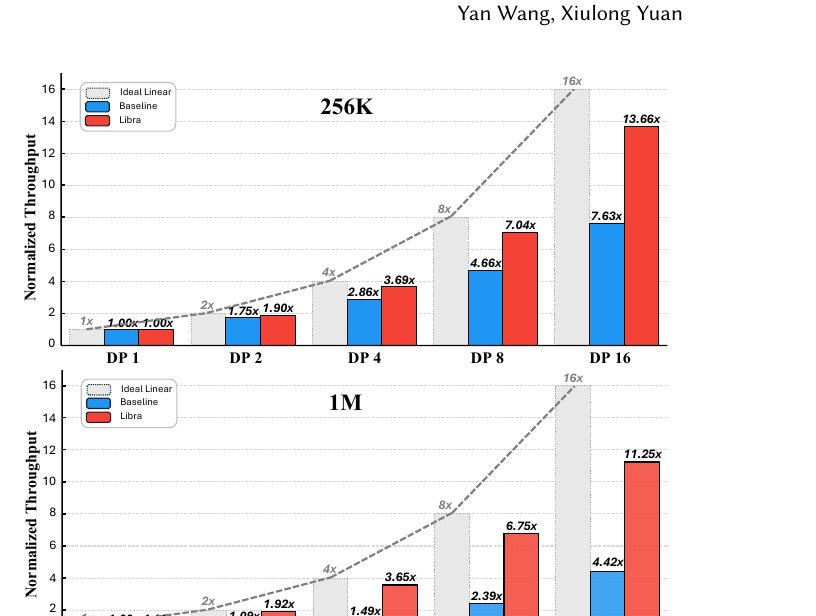
This translates to an end-to-end speedup over the Ulysses baseline of 1.79x on the 256K dataset and 2.54x on the 1M dataset, both at DP=16. The paper offers a clean explanation for why the 1M dataset benefits more: longer sequences produce a heavier attention-FLOPs tail (recall the quadratic proxy from Section 3), so the inter-rank imbalance TAP has to absorb is more severe on 1M, and correspondingly there is more headroom for Libra to recover.

The teaser figure from the paper’s abstract makes the same point at a slightly different DP range (DP 1 to 8, 1M dataset), and is worth including because it’s the figure the authors chose to lead with:

8.3 Pipeline-parallel bubbles: the per-microbatch view

A second, complementary experiment runs pipeline-parallel training and measures the distribution of per-microbatch forward time across 15 iterations, normalized so Libra’s own mean sits at 1.0:

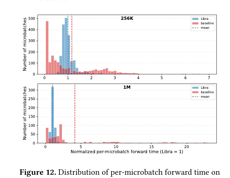
The baseline’s distribution (red) is extremely dispersed — on the 1M dataset it spans 0.02 to 23.1 with a mean of 4.14, while Libra (blue) compresses this to a tight 0.52-1.57 range. Since a pipeline’s bubble size is set by its slowest microbatch in a window (every other stage waits for it), this compression is what actually matters operationally: Libra cuts the worst-case microbatch time from 23.1 to 1.57 on the 1M dataset, a 14.7x reduction, and from 6.98 to 2.63 on 256K (2.6x). The paper is careful to frame this as “indirect evidence” for reduced pipeline bubbles — no actual pipeline trace with bubble measurements is collected in this experiment, only the underlying forward-time distribution that would determine bubble size under a bulk-synchronous pipeline schedule. This is a reasonable proxy, but it stops short of a direct bubble-time measurement, which would have been a stronger and more literal claim.

8.4 Microbenchmarks: isolating the core-attention layer

To compare directly against all three baselines (Ulysses, WLB-LLM, DistCA) without the confound of a full training pipeline, the paper isolates just the core-attention layer and measures per-step straggler latency (the slowest worker’s time), reporting both the mean (proxying throughput impact) and the max (proxying the PP-bubble impact) across a GBS window:

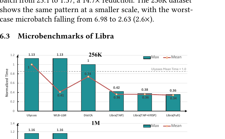
On the 256K dataset, Libra(Full) lowers mean latency by 15.9% versus WLB-LLM and 53.7% versus DistCA, and lowers max latency by 68.4% and 64.2% respectively; against Ulysses, the reductions reach 65.6% (mean) and 68.3% (max). The paper diagnoses why each baseline falls short: WLB-LLM balances the mean reasonably well, but its max stays within 0.2% of Ulysses — because its indivisible outlier packed sequences (recall Section 2.3’s step-equivalence constraint means WLB-LLM in this reproduction cannot defer outliers to later steps) still bottleneck its single slowest step, no matter how well the rest of the batch is balanced. DistCA balances globally (since its pool spans the entire cluster) but trails on the mean because a cluster-wide pool exchanges tiles across all participating GPUs, inflating communication cost — exactly the trade-off flagged analytically back in Section 3.3. Taken together across both datasets, Libra achieves a mean-straggler speedup of 2.91x (256K) / 2.57x (1M) and a worst-step straggler speedup of 3.14x (256K) / 2.90x (1M) over Ulysses.

8.5 Pool-size sweep and component ablation

Sweeping the pool size $P \in \{2,4,8,16,32\}$ (Figure 14 in the paper) with a computation/communication breakdown per component reveals the pattern predicted analytically in Section 3.3 and Section 6.3: communication cost climbs steeply with pool size (on 256K, communication rises from 0.07 normalized time at $P=4$ to 0.17 at $P=8$, 0.47 at $P=16$, and 0.77 at $P=32$), while VRSP’s contribution to reducing computation time is fairly stable across pool sizes once enabled (cutting computation by roughly 23-34% versus TAP-alone, depending on dataset and $P$). The Pipeliner’s overlap hides a growing absolute amount of communication as pool size grows, but the fraction hidden and the residual unhidden leftover both grow with pool size too — confirming the paper’s own boundary condition from Section 6.3 that overlap mitigates, but cannot eliminate, the extra communication a larger pool introduces. Interestingly, the paper reports that $P=4$ slightly edges out $P=8$ in Libra(Full)‘s absolute latency on both datasets, yet the paper still uses $P=8$ throughout the main evaluation — because it was the value the offline simulator (Section 7) selected based on the estimated balance-communication trade-off, not a value chosen by sweeping measured latency after the fact. This is a small but genuine inconsistency worth flagging (discussed further in Section 9).

A separate grid search over TAP’s two granularity knobs — block size $B$ and head-split count $H$ — confirms the head-axis-splitting argument from Section 5.1 empirically: at an equal total tile count, splitting along heads outperforms splitting along the sequence axis on the 256K dataset (1.89x speedup vs. 1.76x at 128 tiles), because all query tiles sharing one KV group can amortize that KV group’s fetch cost over more query work when blocks are larger and heads are split instead. This benefit is pronounced on 256K (which has $h_{kv}=16$) but comparatively small on 1M (which has only $h_{kv}=4$), and the benefit reverses slightly once $H$ exceeds $h_{kv}$ (head shards start sharing expanded KV heads, inflating KV traffic) — a concrete, measured boundary on how far head-splitting can be pushed.

9. Limitations and boundary conditions

The paper is unusually forthright about its own scope, and it is worth collecting these self-disclosed limitations in one place, alongside a few this reviewer would add:

• Scope restricted to dense causal self-attention. The paper explicitly states “balancing sparse or linear attention variants is left to future work.” Given how much production inference (and increasingly training) work is moving toward sparse attention patterns, this is a real and acknowledged gap — the FLOPs proxy (Equation 1), the SH-Tile FLOPs estimate (Equation 8), and the head-axis-splitting argument (Section 5.1) would all need rederivation for sparse masks, where the causal-triangular counting no longer applies cleanly.

• No end-to-end comparison against WLB-LLM or DistCA. The paper is explicit that it only compares against these two baselines in the microbenchmark setting, not end-to-end, because “applying them end-to-end would require invasive modifications to the training framework’s execution scheduling.” This is a reasonable engineering constraint, but it does mean the headline end-to-end numbers (1.79x/2.54x speedup, Section 8.2) are only directly measured against Ulysses — we do not know how WLB-LLM or DistCA would actually perform end-to-end on the same Qwen3-Turbo training job, only how they perform on an isolated attention microbenchmark. The paper’s own indirect argument (recovering most of the lost DP-scaling gap) is offered as “complementary, indirect evidence,” not a substitute for a direct measurement.

• DistCA is emulated, not run as published. The paper states plainly: “we do not run its public implementation; instead, we emulate its balancing scope in our own harness.” This isolates the effect of balancing scope cleanly (which is the paper’s specific interest), but it also means the DistCA numbers in this paper should not be read as a faithful reproduction of DistCA’s full system — DistCA’s token-level dispatch, dedicated attention-server pool, and ping-pong execution co-design are explicitly “not covered” by this emulation. A reader citing this paper’s DistCA numbers as “DistCA’s measured performance” would be over-extending what was actually measured.

• WLB-LLM reproduction deliberately weakens its strongest mechanism. The paper’s reimplementation of WLB-LLM “excludes the outlier-deferral mechanism” specifically because that mechanism would violate the step-equivalence requirement Libra itself adheres to. This is a defensible, principled choice (comparing methods on equal semantic footing), but it does mean the WLB-LLM baseline shown here is not WLB-LLM at its full published strength — it is WLB-LLM minus its key trick for handling indivisible outliers, which unsurprisingly then fails to control the worst-case max latency (Section 8.4). A more charitable framing would have been to additionally report vanilla WLB-LLM’s numbers with deferral, explicitly labeled as violating step-equivalence, so readers could judge both the performance gap and the semantic trade-off Libra is declining to make.

• No wall-clock convergence or model-quality comparison. The paper states training “converges normally in production” and explicitly disclaims bitwise-equivalent gradients or trajectories relative to a non-Libra baseline, but it does not present any loss curves, downstream evaluation scores, or convergence-speed comparison between Libra-trained and baseline-trained checkpoints. For infrastructure changes that alter floating-point operation order, even a brief loss-curve overlay would have meaningfully strengthened the “preserves training semantics” claim beyond “we deployed it and nothing broke.”

• Simulator-selected configuration is not latency-validated. As flagged in Section 8.5, the paper’s own pool-size sweep shows $P=4$ slightly beating $P=8$ in measured Libra(Full) latency, yet $P=8$ is used throughout the main results because the offline simulator selected it based on estimated FLOPs/communication trade-offs. This is a minor inconsistency: the paper builds a whole configuration-simulation apparatus (Section 7) specifically to avoid expensive latency sweeps, but its own sweep (done for the ablation study) suggests the simulator’s choice may be very slightly, though not substantially, suboptimal at these two data points. It would strengthen the paper to explain why $P=8$ was kept despite this, or to note this gap as a known simulator-accuracy limitation.

• Single hardware/interconnect configuration. All experiments run on one NVLink-intra-node/RoCE-inter-node cluster configuration. The paper’s own argument for bounded pools rests partly on communication-domain locality (Section 3.3), so results could plausibly look different on clusters with different intra-node/inter-node bandwidth ratios (e.g., all-NVSwitch full-mesh clusters with less severe inter-node penalties might tolerate somewhat larger pools before the communication-cost argument bites as hard) — the paper does not explore this sensitivity.

Concrete, specific improvement suggestions

1. Add a direct end-to-end comparison against at least one alternative (even a partial/limited-scope integration of WLB-LLM or a smaller-scale DistCA-style disaggregation), rather than relying entirely on microbenchmark comparisons plus an indirect “recovers most of the DP-scaling gap” argument for the end-to-end numbers.
2. Report a loss-curve or downstream-eval comparison between a Libra-trained checkpoint and a non-Libra baseline checkpoint at matched token budgets, to substantiate “preserves training semantics” with more than an operational “no incidents” claim.
3. Publish a small $M$-sweep for the Pipeliner (Section 6.3) and a brief justification for the $P=8$-despite-$P=4$-being-slightly-faster choice (Section 8.5) — both are one-paragraph additions that would close small but noticeable gaps between the paper’s own ablation data and its main-line configuration choices.
4. Extend the FLOPs proxy and SH-Tile design to at least one sparse-attention pattern (even a simple fixed-window or block-sparse case), since sparse attention is increasingly common in exactly the long-context regime this paper targets, and the current proxy (Equation 1, Equation 8) is derived specifically for dense causal masks.

10. Conclusion

Libra’s real contribution is not a new attention kernel or a clever new masking scheme — it reuses an unmodified variable-length FlashAttention kernel throughout. Its contribution is a scheduling and workload-placement discipline, motivated by one clean statistical insight: when redistributing an imbalanced workload across a growing cluster, the redistribution domain does not have to grow with the cluster. The law of large numbers tells you how large a fixed domain needs to be for a given target concentration; you then scale out by adding more fixed-size domains, not by growing existing ones. VRSP supplies the finite-window placement mechanism that makes fixed pools work well in practice (despite long-tailed, non-asymptotic corpora), TAP handles the residual intra-pool imbalance via sequence-and-head tiling, and the Pipeliner claws back most of the resulting communication cost through head-axis-chunked overlap.

The production numbers back this up convincingly: 1.79x-2.54x end-to-end throughput improvement, DP=16 scaling efficiency recovered from 27.6% to 70.3% on the hardest (1M-token) workload, and hundreds of thousands of production GPU-hours without correctness incidents. For anyone building or operating long-context LLM training infrastructure, this paper’s core scaling principle — fixed-size, statistically-justified redistribution domains rather than cluster-wide disaggregation — is a pattern worth internalizing well beyond the specific case of attention load balancing.

11. Reproducibility notes

• Code availability: the paper does not state that Libra’s implementation will be open-sourced; no repository link is given in the arXiv preprint as of this writing. This limits independent reproduction of the exact numbers reported.
• Datasets: both evaluation datasets (256K-token and 1M-token production corpora) are internal/proprietary Alibaba training data; the length-distribution statistics (median, p75, p99) are reported in Figure 2, which is enough to characterize the corpus shape but not to reconstruct it exactly.
• Model: Qwen3-Turbo (Qwen3-30B-A3B) is a real, named model, which aids interpretability of the results, though the specific training configuration (learning rate schedule, optimizer hyperparameters, total training tokens) beyond the parallelism dimensions discussed is not fully specified.
• Key hyperparameters given explicitly in the paper: pool size $P=8$ (both datasets), Pipeliner chunk count $M=4$ (all experiments), placement slack $\tau=0.03$ (all configurations), plus the per-experiment $(CP, DP, GBS)$ settings quoted throughout Section 8 — these are sufficient to attempt a re-implementation on an equivalent Megatron-LM-style stack with a comparable long-tailed long-context corpus, even without the exact original dataset.
• Baselines’ reproducibility status: Ulysses is a published, well-known open-source method (DeepSpeed Ulysses) and should be straightforwardly reproducible; WLB-LLM and DistCA are both reimplemented/emulated by the authors rather than run from official releases, per the caveats in Section 9 above.