Branching Policy Optimization: Turning Sandbox Snapshots Into a Variance-Reduction Primitive

Review date: 2026-07-28 Review author: Zhongzhu Zhou Paper reviewed: Branching Policy Optimization: Sandbox-Native Language Agent Reinforcement Learning Paper authors: Bowei He, Yankai Chen, Xiaokun Zhang, Xue Liu (MBZUAI, McGill University, City University of Hong Kong) arXiv: 2607.14171v1, 2026-07-15 Venue/status: Accepted by WAIC Academic 2026

0. Why this paper is worth a careful read

Most of the recent progress narrative in LLM agent RL reads like a sequence of small simplifications to PPO: drop the critic (RLOO), normalize by group statistics instead of a learned baseline (GRPO), tweak the reward shaping (RAFT, ReST). These are all “loss-level” changes — they keep the same rollout topology inherited from RLHF, where for a given prompt you sample $N$ independent trajectories from scratch and subtract their mean return as a baseline.

Branching Policy Optimization (BPO) asks a different, more structural question: agent training almost always happens inside a sandbox — a Docker container, a browser session, a text-adventure simulator — and sandboxes have a property that a static RLHF preference prompt never had: they can be snapshotted and restored. If you can freeze the sandbox at an intermediate state and fork multiple continuations from there, you don’t have to treat every rollout as an independent sample from the initial state. You can build a tree of rollouts that share a prefix, and that shared prefix carries information you can exploit statistically.

This is the kind of idea that sounds almost too simple once stated, and that simplicity is exactly why it’s worth reading carefully: the paper backs the intuition with two clean theorems (unbiasedness and a closed-form variance-reduction guarantee), ties the reduction explicitly to the law of total variance, and validates all of it on three genuinely different sandboxes (WebShop, ALFWorld, SWE-bench Verified) with two model backbones. The empirical story — 3.6 to 6.1 point absolute gains at matched compute, roughly half the gradient-norm variance throughout training, and a 38% reduction in gradient steps to match GRPO’s final performance — is the kind of result that, if it replicates, changes how people think about designing RL algorithms for agents versus RLHF. This review works through the theory, the algorithm, the experiments, and where the idea is likely to break.

1. Prerequisites

1.1 Policy gradients and baselines, briefly

Reinforcement learning for language models optimizes $J(\theta) = \mathbb{E}_{\tau \sim \pi_\theta}[R(\tau)]$, the expected return of a policy $\pi_\theta$ over trajectories $\tau$. The policy gradient theorem gives:

$$\nabla_\theta J(\theta) = \mathbb{E}_{\tau \sim \pi_\theta}\left[\sum_{t=0}^{T} \nabla_\theta \log \pi_\theta(a_t \mid s_t) \cdot A(s_t, a_t)\right] \tag{1}$$

where $A(s_t, a_t) = Q^\pi(s_t, a_t) - V^\pi(s_t)$ is the advantage: how much better action $a_t$ is than the policy’s average behavior at state $s_t$. The gradient estimator in Eq. (1) is unbiased for any function $A'$ satisfying $\mathbb{E}[A' \mid s_t, a_t] = A$ — the raw return $R(\tau)$ itself is one (very high-variance) choice, and the entire “baseline design” literature is about finding lower-variance substitutes that are still unbiased.

Why does variance matter so much here? Because gradient noise directly slows convergence and can destabilize training (the reason PPO clips instead of doing vanilla policy gradient). For long-horizon agent tasks — a 50-step WebShop episode, or a multi-tool-call SWE-bench trajectory — a single early misstep can flip the terminal reward from 1 to 0, so the return $R(\tau)$ conditioned only on the prompt has very high variance. Reducing that variance without introducing bias is the central engineering problem this whole family of algorithms is solving.

1.2 From REINFORCE to RLOO and GRPO

Vanilla REINFORCE uses $A = R(\tau)$ directly — extremely noisy, because it doesn’t subtract off any baseline. PPO fixes this by learning a critic $V_\phi(s_t)$ and using Generalized Advantage Estimation (GAE), but training a good critic for LLMs is itself expensive and can be unstable in the sparse-reward, long-horizon regime.

The “baseline-only” family (RLOO, GRPO) sidesteps the critic entirely by sampling $N$ independent rollouts $\tau^{(1)}, \ldots, \tau^{(N)}$ from the same initial state $s_0(x)$ for a given prompt $x$, and using the empirical mean (or leave-one-out mean) of their returns as the baseline:

$$A^{\text{GRPO}}_i = \frac{R^{(i)} - \mu_R}{\sigma_R}, \qquad \mu_R = \frac{1}{N}\sum_j R^{(j)}, \quad \sigma_R^2 = \frac{1}{N}\sum_j (R^{(j)} - \mu_R)^2 \tag{2}$$

RLOO uses the un-normalized leave-one-out variant (excluding sample $i$ from its own baseline). Both are unbiased and both are cheap (no critic network), which is why they’ve become the default for agent RL post-DeepSeekMath and DeepSeek-R1. But notice the structural assumption buried in Eq. (2): the baseline conditions only on $s_0$, and every step of trajectory $i$ gets the same scalar advantage. All the variance internal to how the trajectory unfolds after $s_0$ — every branching decision at every intermediate state — is lumped into the return’s variance and left unreduced.

1.3 Sandboxes and the checkpoint-restore primitive

The paper’s core technical lever is a property most RLHF settings don’t have but almost all agent settings do: the environment is a sandbox — a stateful, resumable Markov Decision Process. Concretely, this means there exist two operators:

• $\text{snap}: \mathcal{S} \to \Sigma$ — take a state $s$ and produce an opaque snapshot $\sigma$ (e.g., a Docker overlayfs diff, a CRIU checkpoint, a Python interpreter pickle, a browser session export).
• $\text{rest}: \Sigma \to \mathcal{S}$ — restore a snapshot back into a live state that behaves identically to the original.

The paper formalizes the fidelity requirement as an explicit assumption:

Assumption 1 (Snapshot fidelity). For every state $s$ encountered along an on-policy trajectory, $\text{rest}(\text{snap}(s))$ produces a state with identical transition distribution to $s$.

This is doing real work: it says that once you fork a snapshot and take a different action, the sandbox will behave exactly as if you’d taken that action from the “real” trajectory at that point — no leakage, no drift, no partial state corruption. Everything downstream (the unbiasedness theorem in particular) depends on this holding. WebShop, ALFWorld, and Docker-backed SWE-bench containers all satisfy it reasonably well because their dynamics are either purely deterministic code or a simulator with an explicit, serializable state object.

1.4 Shannon entropy as an uncertainty signal

The paper’s branch scheduler uses per-step policy entropy to decide where in a trajectory to fork additional rollouts:

$$H_t = -\sum_{a \in \mathcal{A}} \pi_\theta(a \mid s_t) \log \pi_\theta(a \mid s_t) \tag{3}$$

Intuitively, $H_t$ is large when the policy is genuinely unsure what to do next (many actions have comparable probability) and small when it is confident (probability mass concentrated on one action). If you’re going to spend a limited branching budget on re-sampling actions from a state, spending it where the policy is already nearly deterministic wastes the budget on near-duplicate rollouts; spending it where the policy is uncertain maximizes the spread of outcomes you get to compare.

2. Architecture and rollout-tree overview

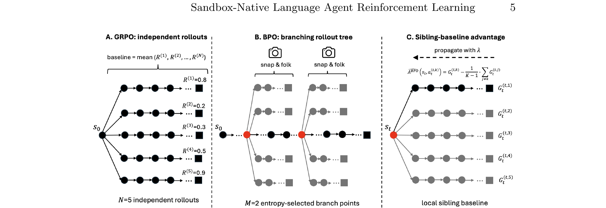
Figure 1 (paper Fig.1): Panel A shows GRPO’s independent-rollout topology — $N=5$ separate paths from $s_0$, each producing a terminal return $R^{(i)}$, with the baseline computed as their mean. Panel B shows BPO’s branching topology: a single backbone trajectory, with $M=2$ entropy-selected branch points (red dots) where the sandbox is snapshotted (“snap & fork”) and $K$ sibling continuations are rolled out. Panel C zooms into one branch point: the sibling-baseline advantage is computed locally among the $K$ siblings, then propagated backward along the shared prefix with discount $\lambda$.

The diagram is the clearest way to internalize the idea. GRPO’s tree is “flat and wide” — $N$ separate root-to-leaf paths that never touch each other after $s_0$. BPO’s tree is “narrow at the root, bushy at a few chosen depths” — one backbone path, and at a handful of high-entropy steps, the sandbox is frozen and forked into $K$ siblings that share everything before the branch point and diverge only after it.

The key structural insight, made precise in §3 below, is: siblings that share a long prefix have already “used up” the variance attributable to that prefix. Their remaining variance is only the variance of the return given the branch state $s_t$ — which the law of total variance guarantees is smaller (often much smaller) than the variance of the return given only $s_0$.

2.1 The training data-flow, end to end

flowchart TD
    A["Prompt x sampled from batch"] --> B["Sample backbone trajectory in sandbox E"]
    B --> C["Compute per-step entropy H_t at each decision boundary"]
    C --> D["Select top-M branch points, min spacing Delta_min"]
    D --> E["For each branch point t: snapshot sandbox state s_t"]
    E --> F["Fork K-1 siblings: restore, sample new action, roll out to termination"]
    F --> G["Compute leave-one-out sibling-baseline advantage per branch point"]
    G --> H["Propagate advantage to pre-branch steps with discount lambda"]
    H --> I["PPO-clip gradient update on whole tree"]
    I --> B

Figure (self-drawn): the end-to-end BPO data flow for one gradient step. The loop from the gradient update back to sampling a fresh backbone captures that this whole procedure repeats every training iteration; nothing here persists across iterations except the policy weights themselves — snapshots are ephemeral and discarded once their sibling rollouts complete.

3. Formalizing the sibling-baseline advantage

3.1 The rollout tree

For a prompt $x$, BPO constructs a rooted tree $\mathcal{T}_x$ with root $s_0(x)$:

1. A backbone trajectory $\tau^{(0)} = (s_0, a_0, s_1, \ldots, s_{T_0}, a_{T_0})$, sampled by running $\pi_\theta$ to termination — this is just a normal on-policy rollout.
2. At each branch point $t \in \mathcal{B} \subseteq \{0, \ldots, T_0-1\}$ (chosen by the entropy scheduler, §4 below), $K-1$ sibling sub-trajectories $\{\tau^{(t,k)}\}_{k=2}^{K}$, obtained by snapshotting $s_t$, restoring it, sampling a fresh action $a_t^{(t,k)} \sim \pi_\theta(\cdot \mid s_t)$, and rolling out to termination. The original backbone action $a_t^{(t,1)} := a_t$ is treated as the first of the $K$ siblings — so the backbone isn’t wasted, it’s reused as sibling #1.

Write $G_t^{(t,k)}$ for the return-to-go of sibling $k$ starting from branch point $t$ (i.e., the discounted sum of rewards from $t$ onward along that sibling’s continuation).

3.2 The sibling-baseline advantage: derivation

At a branch point $t$, BPO computes a leave-one-out baseline over the $K$ siblings only (not over the whole batch of prompts, and not conditioned on $s_0$):

$$\hat{A}^{\text{BPO}}\left(s_t, a_t^{(t,k)}\right) := G_t^{(t,k)} - \frac{1}{K-1}\sum_{j \neq k} G_t^{(t,j)} \tag{4}$$

This is structurally identical to RLOO’s leave-one-out formula — the difference is entirely in what the samples are conditioned on. RLOO’s $K$ samples are $K$ independent rollouts from $s_0$; BPO’s $K$ samples are $K$ rollouts that all share the prefix $s_0 \to \cdots \to s_t$ and only diverge from $s_t$ onward. That shared prefix is the entire source of the variance reduction, derived formally in §3.4.

For steps $t' < t$ that lie before the branch point (i.e., on the shared prefix), there’s no local sibling comparison available — a single prefix step feeds into multiple downstream branch points, potentially at different depths. BPO handles this by propagating the branch-point advantage backward with a discount $\lambda \in (0, 1]$:

$$\hat{A}^{\text{BPO}}(s_{t'}, a_{t'}) := \sum_{t \in \mathcal{B}(\tau)} \lambda^{\,t - t'} \cdot \hat{A}^{\text{BPO}}_{\text{local}}\left(s_t, a_t^{(t, k(\tau))}\right) \tag{5}$$

where $\tau$ is the unique path through the tree containing $(s_{t'}, a_{t'})$, $\mathcal{B}(\tau)$ are the branch points on that path at depth $\geq t'$, and $k(\tau)$ is the sibling index that path corresponds to. Intuitively: a pre-branch action gets credit (or blame) for every downstream branch-point comparison it eventually leads to, discounted by how far downstream that comparison happened. $\lambda = 1$ means full, undiscounted propagation of every downstream sibling comparison; $\lambda \to 0$ collapses to “only the branch point itself gets a nonzero advantage, everything upstream gets zero” — which throws away information but is the simplest possible choice.

Why a discount at all, rather than just $\lambda=1$? The paper’s ablation (§7 below) shows a broad plateau for $\lambda \in [0.9, 0.99]$ and a small but consistent loss at $\lambda=1$ on the longest-horizon environment (SWE-bench), which the authors attribute to long-horizon credit assignment benefiting from some temporal decay — the further back an action is from the actual comparison that revealed information about it, the less directly relevant that comparison should be to updating it. This is the same intuition behind GAE’s $\lambda$, applied here to a different quantity (whether to propagate a sibling comparison, rather than whether to bootstrap a value estimate).

3.3 The full training objective

BPO plugs the advantages of Eq. (4)–(5) into the standard PPO-clip objective, summed over every $(s,a)$ pair in the tree:

$$\mathcal{L}^{\text{BPO}}(\theta) = -\mathbb{E}_{\mathcal{T}_x}\left[\sum_{(s,a) \in \mathcal{T}_x} \min\Big(\rho_\theta(s,a)\hat{A},\ \text{clip}(\rho_\theta(s,a), 1-\epsilon, 1+\epsilon)\hat{A}\Big) + \beta\, \text{KL}(\pi_\theta \Vert \pi_{\text{ref}})\right] \tag{6}$$

where $\rho_\theta(s,a) = \pi_\theta(a\mid s)/\pi_{\theta_{\text{old}}}(a\mid s)$ is the usual importance ratio. One subtlety worth flagging explicitly (the paper notes it but doesn’t dwell on it): because every $(s,a)$ pair in the tree contributes a term to the sum, and shared-prefix states appear only once per tree but influence multiple downstream leaves, the effective gradient weight on a shared-prefix action is implicitly higher than on a leaf-only action — the paper calls this an “advantage-broadcast” effect that is structurally impossible in trajectory-flat algorithms like GRPO, where every state appears in exactly one trajectory.

3.4 Why the variance actually goes down: the law of total variance

This is the theoretical core of the paper, and it’s worth deriving in full rather than taking on faith. Fix a branch point $t > 0$ and a budget of $K$ return samples for the advantage estimate, in one of two configurations:

• GRPO/RLOO: $K$ independent rollouts $\tau^{(1)}, \ldots, \tau^{(K)}$ all starting from $s_0$, giving i.i.d. returns $G^{(1)}, \ldots, G^{(K)}$.
• BPO: $K$ sibling rollouts sharing the prefix $\tau_{0:t}$, forking only from $s_t$ onward, giving returns $G_t^{(t,1)}, \ldots, G_t^{(t,K)}$ that are i.i.d. conditional on $s_t$, but not unconditionally i.i.d. (they share the randomness of how the trajectory got to $s_t$).

Step 1 — decompose the unconditional variance of the return using the law of total variance. For any random variable $G$ that depends on the path through $s_t$:

$$\text{Var}(G \mid s_0) = \underbrace{\mathbb{E}\big[\text{Var}(G \mid s_t)\big]}_{=:\ \sigma_t^2} + \underbrace{\text{Var}\big(\mathbb{E}[G \mid s_t]\big)}_{=:\ \nu_t^2 \ =\ \text{Var}(V^\pi(s_t))} \tag{7}$$

The first term, $\sigma_t^2$, is the residual variance that remains even after you know exactly which state $s_t$ you ended up in — it’s the “genuinely random” part of what happens after $t$. The second term, $\nu_t^2$, is the variance of the conditional mean itself — i.e., how much the expected return $V^\pi(s_t) = \mathbb{E}[G \mid s_t]$ varies depending on which particular prefix $\tau_{0:t}$ you happened to sample. This is exactly the quantity that a trajectory-flat estimator like GRPO cannot see, because it never conditions on anything past $s_0$.

Step 2 — compute GRPO’s leave-one-out variance. The $K$ returns are i.i.d. with variance $\sigma_t^2 + \nu_t^2$ (the total variance from Eq. 7, since they’re unconditionally i.i.d.). For i.i.d. samples, the leave-one-out advantage $A_k = G^{(k)} - \frac{1}{K-1}\sum_{j\neq k} G^{(j)}$ has variance:

$$\text{Var}(A_k^{\text{GRPO}}) = \frac{K}{K-1}\left(\sigma_t^2 + \nu_t^2\right) \tag{8}$$

(This is a standard fact about leave-one-out statistics of i.i.d. variables: $\text{Var}(X - \bar{X}_{-i}) = \text{Var}(X)(1 + \frac{1}{K-1}) = \frac{K}{K-1}\text{Var}(X)$.)

Step 3 — compute BPO’s leave-one-out variance. Conditional on $s_t$, the $K$ siblings are i.i.d. with variance $\text{Var}(G \mid s_t) = \sigma_t^2$ (by definition), and by the leave-one-out symmetry, $\mathbb{E}[A_k^{\text{BPO}} \mid s_t] = 0$ for every sibling. So, applying the tower rule (average the conditional variance over the randomness in $s_t$, plus the variance contribution of the conditional mean, which is zero here because the conditional expectation of $A_k$ given $s_t$ is identically zero):

$$\text{Var}(A_k^{\text{BPO}}) = \mathbb{E}_{\tau_{0:t}}\left[\frac{K}{K-1}\text{Var}(G \mid s_t)\right] + 0 = \frac{K}{K-1}\sigma_t^2 \tag{9}$$

Step 4 — subtract. Comparing Eq. (8) and Eq. (9):

$$\text{Var}(A_k^{\text{GRPO}}) - \text{Var}(A_k^{\text{BPO}}) = \frac{K}{K-1}\nu_t^2 \geq 0 \tag{10}$$

with equality only if $\nu_t^2 = 0$, i.e., only if $V^\pi(s_t)$ happens to be constant across all prefixes — which for any nontrivial task means BPO’s variance is strictly lower whenever the value function actually varies across trajectories (which is exactly when a baseline is useful in the first place). This is Theorem 2 in the paper; the proof structure above matches theirs, spelled out with the intermediate algebra filled in.

Intuition in one sentence: GRPO’s baseline can only remove the variance attributable to “which prompt did you get,” while BPO’s sibling baseline additionally removes the variance attributable to “which prefix did the backbone happen to wander into before branching” — and for long, high-stakes agent trajectories, that second source often dominates the first.

A corollary worth internalizing: the paper also shows (Corollary 1) that branching deeper into the trajectory yields a larger reduction than branching shallow, because $\nu_t^2 = \text{Var}(V^\pi(s_t))$ tends to grow with $t$ — the further into a trajectory you are, the more the value function has had a chance to diverge across different paths (an early WebShop search query barely constrains the eventual outcome; a near-checkout state constrains it a lot). This directly motivates favoring branch points later rather than earlier in the trajectory, all else equal — though the entropy scheduler (next section) can still override this if early steps happen to be high-entropy.

3.5 A worked toy numerical example

Abstract variance formulas are easy to nod along with and hard to actually feel. Here’s a small worked example with made-up but internally consistent numbers, to make Eq. (7)–(10) concrete.

Suppose a WebShop-style task has a branch point $t$ at the moment the agent has just picked a product category, three steps before the end of the episode. Say there are two “kinds” of prefix the backbone could have wandered into by step $t$: a good prefix (the agent picked a category that matches the instruction well) and a bad prefix (a near-miss category). Assume, for the sake of a clean number:

• With probability $\frac{1}{2}$, the backbone lands in a good prefix, from which $V^\pi(s_t) = 0.8$ (i.e., conditional on being in a good prefix, the expected eventual return is 0.8), and the residual variance of the return given this prefix is $\text{Var}(G \mid s_t) = 0.05$.
• With probability $\frac{1}{2}$, the backbone lands in a bad prefix, from which $V^\pi(s_t) = 0.2$, with the same residual variance $0.05$.

First compute the pieces of Eq. (7). The residual term is easy since it’s the same in both cases: $\sigma_t^2 = \mathbb{E}[\text{Var}(G\mid s_t)] = 0.05$. The prefix-explained term is the variance of a two-point distribution taking values $0.8$ and $0.2$ each with probability $\frac12$:

$$\nu_t^2 = \text{Var}(V^\pi(s_t)) = \mathbb{E}[V^\pi(s_t)^2] - \big(\mathbb{E}[V^\pi(s_t)]\big)^2 = \frac{0.8^2+0.2^2}{2} - 0.5^2 = 0.34 - 0.25 = 0.09 \tag{11}$$

So the total unconditional return variance seen by GRPO/RLOO at this branch point is $\sigma_t^2 + \nu_t^2 = 0.05 + 0.09 = 0.14$ — and notice that the prefix-explained component ($0.09$) is actually larger than the pure within-prefix noise ($0.05$): most of what GRPO treats as “return variance” here is really just “which prefix did I happen to land in,” not genuine post-branch randomness.

Now plug into Eq. (8)–(9) with $K=4$ siblings, so $\frac{K}{K-1} = \frac{4}{3} \approx 1.333$:

$$\text{Var}(A_k^{\text{GRPO}}) = \frac{4}{3}(0.05+0.09) = \frac{4}{3}(0.14) \approx 0.187, \qquad \text{Var}(A_k^{\text{BPO}}) = \frac{4}{3}(0.05) \approx 0.067 \tag{12}$$

That’s a 64% reduction in advantage variance at this branch point, purely from conditioning on which prefix you’re in rather than pooling across both prefix types as if they were interchangeable. The reduction $\frac{4}{3}\nu_t^2 = \frac{4}{3}(0.09) = 0.12$ matches Eq. (10) exactly. This toy example is deliberately exaggerated (a real WebShop trajectory has more than two discrete prefix “kinds”), but it isolates exactly why the empirical ratio in Figure 3 sits around 0.42–0.58 rather than near 1: whenever a meaningful fraction of return variance is attributable to which prefix you’re in rather than what happens after, sibling-conditioning removes a large chunk of it for free.

4. Algorithm: entropy-driven branch scheduling and the full training loop

4.1 Why entropy, and not a learned value-disagreement signal?

A natural alternative to entropy-based scheduling would be to branch wherever a learned value network disagrees with itself across candidate actions — i.e., estimate $V^\pi$ separately for each of several candidate next actions and branch where those estimates spread out the most. The paper deliberately rejects this design, for two stated reasons:

1. It would require training a value network, which defeats the entire point of the “baseline-only” family (the reason GRPO/RLOO exist is to avoid a critic).
2. Early in training, a value network’s own approximation error would be confounded with genuine value disagreement — you can’t tell whether the network disagrees because the task genuinely has high variance at that point, or because the network just hasn’t learned yet.

Policy entropy, in contrast, is intrinsic to $\pi_\theta$ itself, requires zero extra parameters, and is well-calibrated by construction (a well-trained policy that is genuinely unsure will show it in its own output distribution). The ablation in §7 confirms this design choice empirically: the entropy scheduler comes within 0.6 points of an oracle schedule that gets to peek at a held-out value network at evaluation time only — i.e., entropy alone recovers almost all of the benefit that a “cheating” value-based oracle would get, without paying for a value network at all.

4.2 The scheduler, step by step

1. Run the backbone trajectory to termination, recording every step’s action distribution.
2. Compute Shannon entropy $H_t$ (Eq. 3) at every decision boundary — i.e., at the end of each agent-level action (a completed tool call, a completed reasoning step), not at every individual token. This matters: the unit of “branching” is a semantically meaningful decision point in the agent’s interaction with the sandbox, not an arbitrary token position.
3. Select the top-$M$ decision boundaries by entropy, subject to a minimum spacing constraint $\Delta_{\min}$ (default 64 tokens) — this spacing constraint exists specifically to prevent all $M$ branch points from clustering inside a single high-entropy region (e.g., one long uncertain reasoning span), which would waste budget on near-duplicate branch points that all condition on almost the same prefix.

4.3 Full algorithm

Algorithm 1: BPO training loop (per gradient step)

Require: policy π_θ, reference π_ref, sandbox env E,
         prompt batch {x_i}, branch count M, branch width K,
         propagation discount λ, clip ε, KL weight β

for each prompt x_i in parallel:
    1. Sample backbone trajectory τ_i = (s_0, a_0, ..., s_T0, a_T0) from π_θ in E
    2. Compute step entropies {H_t} for t = 0 .. T0-1   via Eq. (3)
    3. Select branch points B_i ← TopM({H_t}, M, Δ_min)
    4. for each branch point t in B_i:
         a. σ ← snap(s_t)                      # O(c_snap), cheap relative to a rollout
         b. for k = 2 .. K in parallel:
              restore s_t ← rest(σ)
              sample a_t^(t,k) ~ π_θ(· | s_t)
              roll out sibling k to termination, record G_t^(t,k)
    5. Compute branch-point advantages {Â^BPO(s_t, a_t^(t,k))}  via Eq. (4)
    6. Propagate to pre-branch steps                            via Eq. (5)

Update θ ← θ - η ∇_θ L^BPO(θ)   using Eq. (6), aggregated over the whole batch

Three implementation properties the paper highlights as practically important:

1. Compute matching: the total number of sampled returns per prompt is $1 + M(K-1)$ (one backbone rollout, plus $K-1$ siblings at each of $M$ branch points). This is set equal to GRPO’s $N$ in every comparison, so gains can’t be attributed to “BPO just samples more.”
2. Embarrassing parallelism: sibling rollouts within a branch point share nothing after the fork point, so they parallelize trivially across the LLM inference batch and across sandbox worker processes.
3. Bookkeeping is $O(1)$ per step: the only extra state carried per trajectory step is the snapshot handle $\sigma$ and the entropy value $H_t$ — neither scales with trajectory length, which matters for long SWE-bench-style trajectories with 25+ tool calls.

5. Experimental setup

• Environments. WebShop (simulated e-commerce, continuous reward in $[0,1]$, 500-instruction test split, $T_{\max}=50$); ALFWorld (household simulator, 6 task types, 134-task unseen split, $T_{\max}=40$, snapshot via state pickling); SWE-bench Verified (500 real GitHub issues, Docker-per-repo sandbox with overlayfs snapshotting, binary reward from the official test harness, SWE-agent scaffold, $T_{\max}=25$ tool calls).
• Baselines, all reimplemented in the authors’ own codebase for fair comparison: SFT-only, PPO (with a learned critic), RLOO, GRPO, and VinePPO (which the paper treats as its closest relative — see §6 for the comparison discussion).
• Backbones. SFT-initialized Qwen2.5-7B-Instruct for the main results; Llama-3.1-8B-Instruct for a scale/generality check on WebShop.
• Compute matching. GRPO/RLOO/PPO use $N=8$ independent rollouts; VinePPO samples 8 trajectories plus 8 Monte Carlo value rollouts; BPO uses $M=2, K=4$ (giving $1 + 2\cdot 3 = 7$ total returns, an approximate match) in the main comparison, with the exact $N$-matching handled per experiment.
• Optimization. AdamW, learning rate $2\times10^{-6}$, cosine decay, batch size 128 prompts, PPO clip $\epsilon=0.2$, KL weight $\beta=0.05$, propagation discount $\lambda=0.95$, 3 seeds per configuration, 3,000 gradient steps (WebShop/ALFWorld) or 5,000 steps (SWE-bench), 8×A100-80GB per run plus a separate 32-core sandbox worker pool.

6. Design choice: BPO vs. VinePPO — same idea, different mechanism

VinePPO is the paper’s closest relative and deserves a careful side-by-side, because on the surface both methods “use intermediate sandbox states to improve credit assignment,” and it would be easy to conflate them.

What VinePPO does: it replaces PPO’s learned critic with Monte Carlo value estimates — roll out several trajectories from a sampled intermediate state, average their returns, and use that average as a plug-in estimate of $V^\pi(s_t)$ inside a standard Generalized Advantage Estimation (GAE) computation. The intermediate-state rollouts are a value oracle, feeding a conventional actor-critic-style advantage.

What BPO does: it uses the sibling rollouts directly as a leave-one-out baseline, with no GAE and no explicit value estimate ever materialized. The advantage in Eq. (4) is computed purely from returns, never from a fitted or bootstrapped value function.

Two concrete differences fall out of this:

1. No critic-shaped object anywhere. VinePPO’s MC estimate of $V^\pi(s_t)$ still plays the same role a learned critic would play inside GAE — it’s a plug-in replacement, not an architectural change. BPO has genuinely no analogue: the leave-one-out mean over siblings is algebraically an advantage estimator directly, with the value-function-like quantity ($\frac{1}{K-1}\sum_{j\neq k} G_t^{(t,j)}$) appearing only as an intermediate term inside the advantage formula, never estimated or used on its own.
2. Where the sampling budget goes. VinePPO samples states to evaluate uniformly along a trajectory. BPO’s entropy scheduler concentrates budget where the policy is uncertain. The paper’s ablation (Table 3, §7) shows this matters: an inverted (lowest-entropy) schedule actively underperforms GRPO at matched $N$, while the entropy schedule outperforms both GRPO and a uniform-random schedule.

Where might VinePPO’s approach still have an edge? VinePPO’s MC-value-into-GAE pipeline can, in principle, propagate credit through every step of the trajectory using bootstrapped $n$-step returns, which is a more classical and more thoroughly studied machinery than BPO’s ad hoc discount-$\lambda$ propagation (Eq. 5). If the discount-$\lambda$ propagation turns out to be poorly calibrated in some new environment, VinePPO’s GAE-based propagation has decades of RL tooling and diagnostics behind it that BPO’s newer mechanism doesn’t yet have. The empirical results (BPO beats VinePPO by 3.6–4.7 points across all three environments) suggest this isn’t a decisive practical concern for these three benchmarks, but it is a reasonable place to expect BPO’s advantage to narrow on tasks with much longer horizons or much sparser branch-worthy uncertainty.

6.1 Visualizing the variance decomposition

flowchart LR
    subgraph Total["Total return variance given only s_0 (what GRPO sees)"]
        direction TB
        S["sigma_t^2: residual variance after branching (unavoidable)"]
        N["nu_t^2: prefix-explained variance (which prefix did you land in)"]
    end
    Total --> GRPO["GRPO/RLOO advantage variance: K/(K-1) times (sigma_t^2 + nu_t^2)"]
    S --> BPO["BPO advantage variance: K/(K-1) times sigma_t^2 only"]
    N -.->|"removed by sibling conditioning"| BPO

Figure (self-drawn, math-visualizing): a schematic of the law-of-total-variance decomposition from Eq. (7)–(10). GRPO’s baseline only ever sees the combined box on the left; BPO’s sibling conditioning strips out the $\nu_t^2$ piece entirely, leaving only the residual $\sigma_t^2$ term in its advantage variance. The size of the win is exactly how large $\nu_t^2$ is relative to $\sigma_t^2$ for a given task and branch depth — which is why Corollary 1 (deeper branches help more) and the toy example in §3.5 both matter for intuition.

7. Main results and ablations

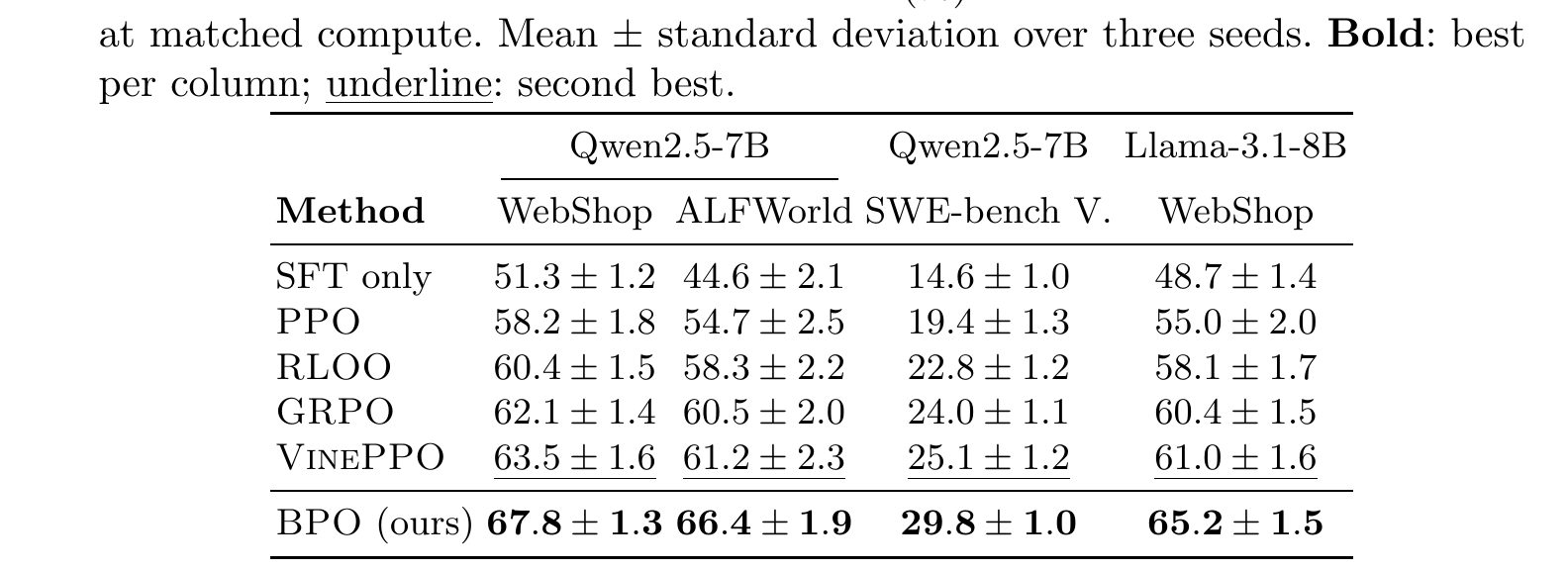
Table 1 (paper Table.1): End-task success rate (%) at matched compute, mean ± std over 3 seeds. BPO is strictly best on every column, with the largest absolute gains on the longest-horizon task (SWE-bench Verified, +4.7 over the best baseline VinePPO) and on ALFWorld (+5.2). The WebShop gain (+4.3) is smaller but still the largest margin in the table relative to the strongest competitor.

A few observations worth pulling out beyond the raw numbers:

• The ranking of baselines is itself informative. SFT-only < PPO < RLOO < GRPO < VinePPO < BPO is a remarkably consistent ordering across all four (environment, backbone) columns. This isn’t surprising in the abstract (more sophisticated credit assignment should help monotonically), but it’s reassuring that the ordering doesn’t flip anywhere — a common failure mode for RL algorithm papers is a method that wins on the primary benchmark but loses on a held-out one.
• The Llama-3.1-8B column is the generality check. BPO’s advantage over GRPO (65.2 vs. 60.4) is essentially unchanged in magnitude from the Qwen2.5-7B WebShop column (67.8 vs. 62.1), suggesting the effect isn’t an artifact of one particular backbone’s training dynamics.

Figure 2 (paper Fig.2): Success rate vs. gradient step, shaded ±1 s.d. over 3 seeds. BPO (red) both reaches a higher plateau and gets there faster than every baseline on all three environments. The vertical dashed line marks the step at which BPO first matches GRPO’s final performance — reported as 1,840 ± 90 steps on average, a 38.7% reduction from GRPO’s full 3,000-step budget. The gap between BPO and the rest is visibly largest in the first 1,000 steps, which the authors attribute to return variance being highest early in training (when the policy is still exploring broadly) — exactly the regime where a variance-reduced estimator should help most.

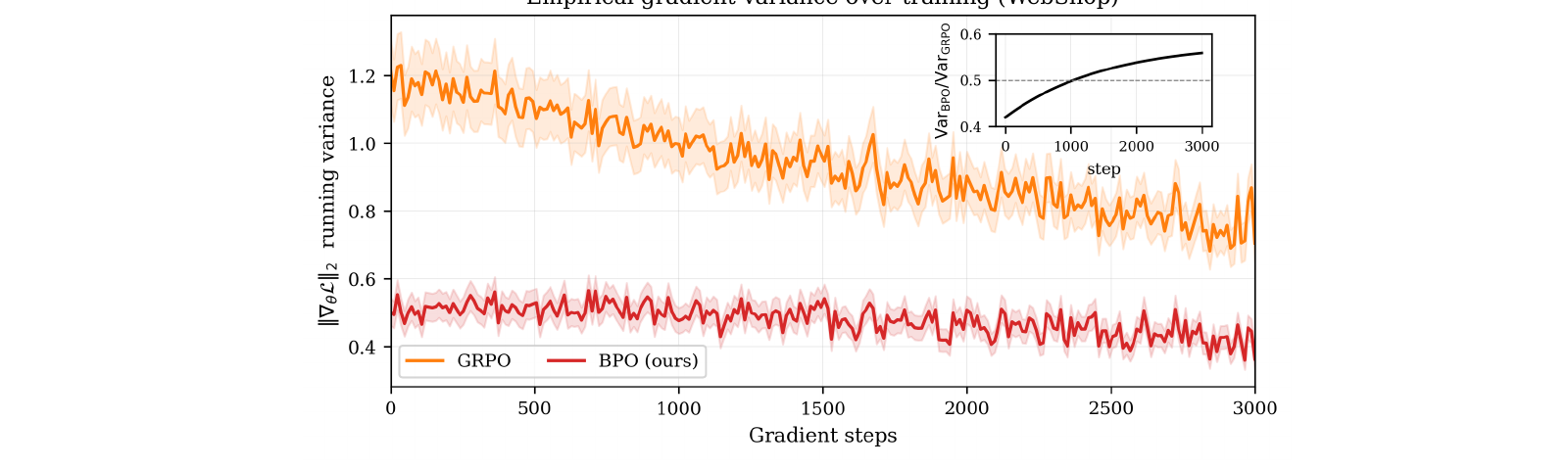
Figure 3 (paper Fig.3): Running variance of the per-mini-batch gradient norm $\|\nabla_\theta \mathcal{L}\|_2$ (window of 50 mini-batches), on WebShop. BPO (red) maintains roughly half the variance of GRPO (orange) throughout training. The inset shows the ratio $\text{Var}_{\text{BPO}}/\text{Var}_{\text{GRPO}}$ climbing from about 0.42 early in training to about 0.58 near convergence — which is exactly the direction Theorem 2 predicts: the reduction term $\frac{K}{K-1}\nu_t^2$ shrinks as the policy converges and $V^\pi(s_t)$ becomes flatter across prefixes (less to gain from conditioning on the branch state once most prefixes lead to similar outcomes anyway).

Branch width ablation (Table 2 in the paper). Sweeping $K \in \{1, 2, 4, 8, 16\}$ at an approximately fixed total return budget ($N \approx 13$): performance rises sharply from $K=1$ (no branching, degenerates to a GRPO-like baseline) to $K=4$, then saturates and even dips slightly at $K=16$ — but the paper is careful to note this dip is an artifact of compute-matching forcing $M$ down to nearly zero branches at $K=16$, not evidence that wide branching is intrinsically bad.

Branching schedule ablation (Table 3). Comparing the entropy scheduler against uniformly-random branch points, equally-spaced branch points, and an inverted (lowest-entropy) schedule: the lowest-entropy schedule actively hurts relative to GRPO at the same $N$ (60.8% vs GRPO’s 62.1%), because branching where the policy is already confident produces near-identical siblings that carry almost no comparative signal. The entropy-based schedule (67.8%) is within 0.6 points of an oracle schedule that gets to use a held-out value-disparity network at evaluation time only (68.4%) — strong evidence that entropy is capturing nearly all of the useful signal a much more expensive value-based oracle would provide.

Why does it actually work, beyond the variance argument? The paper offers two supplementary mechanisms:

1. The fraction of training steps with a “non-degenerate” advantage (defined as $\max|\hat{A}| > 0.1$) rises from 71% under GRPO to 94% under BPO on SWE-bench — meaning far fewer wasted gradient steps where an entire batch of $N$ rollouts happened to all succeed or all fail (giving GRPO a near-zero advantage signal and nothing useful to learn from).
2. Pass@1 improves disproportionately on hard instances (+6.8 points) versus easy ones (+2.1 points), consistent with the idea that sibling-baseline structure matters most exactly where prefix structure is most determinative of the eventual outcome.

7.1 Placing the baseline family on one map

flowchart TD
    PG["REINFORCE: A = R(tau), no baseline"] --> PPO["PPO: learned critic V_phi, GAE"]
    PG --> RLOO["RLOO: leave-one-out mean over N independent rollouts from s_0"]
    RLOO --> GRPO["GRPO: same, plus std-normalization"]
    PPO --> VinePPO["VinePPO: MC value estimate from intermediate states, still feeds GAE"]
    GRPO --> BPO["BPO: leave-one-out mean over K siblings sharing prefix up to branch point t"]
    VinePPO -.->|"closest relative, different mechanism (Sec 6)"| BPO

Figure (self-drawn, baseline/prior-art comparison): where BPO sits relative to the algorithms discussed in this review. The rightward drift from REINFORCE to RLOO/GRPO is “remove the critic, keep independence.” The drift from GRPO to BPO is orthogonal: “keep the leave-one-out estimator, remove the independence assumption by conditioning on a shared prefix instead of only $s_0$.” VinePPO sits in between — it removes the critic’s parameters but keeps a value-estimate-shaped quantity inside a GAE-style computation, which is why §6 treats it as the nearest neighbor rather than a strict ancestor or descendant of BPO.

8. Snapshot overhead: does the theory survive contact with real wall-clock time?

A method that’s provably lower-variance in theory could still lose in practice if the mechanism enabling it (snapshotting) is expensive. The paper measures this directly (Table 4):

Environment	Snapshot cost $c_{\text{snap}}$	Avg rollout length	Branch overhead (% of rollout time)	Wall-clock to match GRPO
WebShop	42 ms	11.4 s	0.6%	8.2 h vs. 13.5 h
ALFWorld	138 ms	9.1 s	2.4%	11.4 h vs. 17.0 h
SWE-bench V.	1,920 ms	182 s	4.2%	47.6 h vs. 74.1 h

Even on SWE-bench, where a Docker/overlayfs snapshot costs nearly 2 seconds — the most expensive case by a wide margin — that overhead is only about 4% of the average rollout duration, because SWE-bench rollouts themselves take 3 minutes on average. The reduction in required gradient steps (38%) dwarfs this overhead, giving a net 35–40% wall-clock training-time reduction across all three environments. This is an important robustness check: it would be easy for a paper to report only the “gradient steps” axis and let readers assume wall-clock savings follow automatically; the explicit measurement here closes that gap.

Design choice: why not report this trade-off as purely a function of snapshot cost in general? Because snapshot cost is environment-specific and implementation-specific (overlayfs vs. CRIU vs. pickling have very different cost profiles), the paper is right to report it per-environment rather than as a single number — but this also means a practitioner adopting BPO in a new sandbox needs to measure their own snapshot cost before assuming the wall-clock benefit will hold. A sandbox with expensive, non-incremental snapshotting (e.g., a full VM image dump rather than a copy-on-write diff) could plausibly erase the benefit; the paper doesn’t test this failure regime.

9. Limitations and boundary conditions

The paper is reasonably upfront about some constraints, and a few more become apparent on close reading:

1. Snapshot fidelity (Assumption 1) is load-bearing and not universally available. Environments with genuine external non-determinism that a snapshot can’t capture (live network calls to a real e-commerce site rather than a simulator, wall-clock-dependent APIs, multi-agent environments where another agent’s state can’t be frozen) violate the assumption outright. The paper tests only environments where this holds cleanly by construction.
2. The propagation discount $\lambda$ is a new hyperparameter with only a loose theoretical justification. Unlike GAE’s $\lambda$, which has a well-understood bias-variance trade-off derivation, Eq. (5)‘s $\lambda$ is motivated primarily by the empirical plateau observed in the ablation, not by a matching theoretical result — the paper proves variance reduction for the local branch-point advantage (Theorem 2) but not for the propagated advantage used at every non-branch step.
3. The compute-matching convention (fixing $N = 1 + M(K-1)$) treats a sibling rollout and an independent rollout as equally expensive, which is true in raw LLM forward-pass cost but not necessarily in wall-clock terms once snapshot/restore overhead and sandbox worker contention are considered at scale — the paper’s own Table 4 shows this overhead is small at the tested batch sizes, but doesn’t stress-test it at much larger $M \cdot K$ or under sandbox-worker-pool contention.
4. All three benchmarks have single-agent, single-objective, verifiable terminal rewards. It’s unclear how the branch scheduler and the sibling-baseline advantage interact with dense, per-step process rewards (rather than sparse terminal rewards) or with multi-agent settings where the “sandbox state” includes another learning agent’s policy.
5. The theory assumes $K$ siblings are drawn from the current policy $\pi_\theta$ at the branch point, but in an off-policy or delayed-update setting (common in large-scale asynchronous RL infrastructure), the siblings might be drawn from a slightly stale $\pi_{\theta_{\text{old}}}$, which the importance-ratio clipping in Eq. (6) partially but not fully compensates for — the paper’s experiments are run synchronously, so this interaction is untested.

10. Critical analysis

Weaknesses and flaws specific to this paper. The headline “matched compute” claim deserves a closer look: BPO’s exact $(M, K)$ configuration used to hit the reported $N$ in the main table (§5, “Compute matching”) is described somewhat loosely in the text — the paper mentions both ”$M=4, K=4$ giving 13 rollouts, sub-sampled to match” and ”$M=2, K=4$ for an exact match at $N=7$” as alternative configurations, without fully specifying which one produced the headline Table 1 numbers. This is a reproducibility gap: a reader trying to replicate Table 1 exactly would need to guess which configuration, or run both and hope they land close. It’s a minor point relative to the overall contribution, but it’s the kind of detail that matters a lot for exact replication and should have been pinned down in a single canonical configuration per row.

Limitations the authors understate or omit. The paper frames snapshot fidelity (Assumption 1) as essentially free for the three tested sandboxes, and indeed it likely holds well for WebShop, ALFWorld, and single-container SWE-bench. But the paper doesn’t discuss the maintenance burden this assumption places on anyone building a new sandbox environment for BPO-style training: guaranteeing that rest(snap(s)) behaves identically to s requires careful engineering discipline (making sure no hidden global state — random seeds not properly threaded through, cached file descriptors, background timers — leaks across a snapshot boundary), and violations of this can be silent: a slightly-off snapshot won’t crash, it will just quietly bias the sibling comparisons in a way that’s very hard to detect from success-rate metrics alone. This risk is understated relative to how central the assumption is to every theoretical guarantee in the paper.

Similarly, the paper’s variance-reduction theory (Theorem 2) is proven for a single branch point in isolation; the multi-branch case is claimed to “follow by induction,” but induction over branch points that all share overlapping prefix segments (since the backbone is one shared path threading through all $M$ branch points) is not entirely trivial — correlations between the advantage estimates at different branch points on the same backbone are not obviously zero, and the paper doesn’t provide the multi-branch proof or bound the covariance terms explicitly. The empirical variance reduction (Figure 3) is consistent with the theory holding up in aggregate, but a reader can’t verify the multi-branch claim from the paper text alone.

Concrete, specific improvement suggestions.

1. Publish the exact $(M, K)$ configuration used for each cell of Table 1, rather than describing two candidate configurations in prose — ideally as a supplementary table alongside the main results, so the compute-matching claim is independently checkable.
2. Provide the multi-branch variance bound (even a looser one with an explicit covariance term) rather than asserting the single-branch result “follows by induction” — this is the one piece of the theoretical apparatus that, as written, a careful reader cannot verify without redoing the derivation themselves.
3. Add an explicit ablation on snapshot fidelity violation — e.g., deliberately inject small amounts of non-determinism into one of the sandboxes (say, a randomized network delay in WebShop) and measure how much the reported gains erode, to give practitioners a concrete sense of how much slack the method has before Assumption 1’s violation becomes a real problem rather than a theoretical footnote.
4. Test at least one dense-reward or process-reward-supervised environment, since sparse terminal-only reward is the one setting where “an early misstep determines a fifty-step outcome” is most acute — it would strengthen the paper considerably to show the sibling-baseline advantage still helps (or characterize when it stops helping) once reward is denser and the baseline-variance problem GRPO has is naturally smaller.
5. Report results at larger model scale (e.g., a 32B or 70B backbone) — all reported backbones are 7–8B; agent RL findings at this scale don’t always transfer cleanly to larger models where entropy calibration and KL behavior can differ substantially.

11. Reproducibility notes

The paper reports enough detail to attempt a careful re-implementation: full hyperparameters (learning rate $2\times10^{-6}$, cosine decay, batch size 128, PPO clip $\epsilon=0.2$, KL weight $\beta=0.05$, $\lambda=0.95$), 3 seeds per configuration with mean ± std reported throughout, exact hardware (8×A100-80GB per run, separate 32-core sandbox pool), and exact benchmark splits (500-instruction WebShop test set, 134-task ALFWorld unseen split, 500-issue SWE-bench Verified). What’s missing for a bit-exact reproduction: the precise $(M,K)$ configuration per Table 1 cell (§10 above), the exact entropy-computation granularity beyond “at decision boundaries” (is entropy computed from the first generated token of the next action, or averaged over the whole action span?), and the sandbox-worker-pool scheduling policy under contention (relevant if a re-implementer doesn’t have 32 dedicated cores available). A careful re-implementer should budget extra time for hyperparameter re-tuning around the branch-width/branch-count trade-off, since Table 2’s ablation shows this interacts non-trivially with the compute-matching convention.

12. Notation reference

Symbol	Meaning
$s_0, s_t$	initial state / state at step $t$ along a trajectory
$\tau^{(0)}$	backbone trajectory
$\mathcal{B}$	set of chosen branch points
$K$	branch width (number of siblings per branch point, including the backbone action)
$M$	number of branch points per prompt
$G_t^{(t,k)}$	return-to-go of sibling $k$ starting from branch point $t$
$\hat{A}^{\text{BPO}}$	sibling-baseline advantage
$\lambda$	propagation discount for pre-branch steps
$H_t$	policy entropy at step $t$, used for branch-point selection
$\sigma_t^2$	residual (within-prefix) return variance at branch point $t$
$\nu_t^2$	prefix-explained return variance ($=\text{Var}(V^\pi(s_t))$) at branch point $t$
$c_{\text{snap}}$	wall-clock cost of one sandbox snapshot operation

13. How this fits the broader agent-RL landscape

It’s useful to place BPO relative to two other lines of work this review has referenced only in passing.

Relative to inference-time tree search (Tree-of-Thoughts, RAP, AlphaZero-style decoding). These methods also exploit a sandbox’s snapshot/restore capability, but purely at inference time, to search for a single better trajectory to execute or to generate higher-quality supervised data (MCTS-DPO, ReST-MCTS$^\star$). They inherit the value-network machinery of AlphaZero, with all its associated complexity (a trained value network guiding the search, careful exploration-exploitation balancing at each node). BPO’s tree is built for a completely different purpose — variance reduction of a training gradient — and deliberately avoids a value network anywhere in the pipeline. The two ideas are complementary rather than competing: nothing prevents combining BPO-style training with tree-search-based inference once training is done, since they touch different parts of the pipeline.

Relative to process reward models (PRMs). Math-Shepherd and similar approaches densify sparse terminal rewards by training a separate model to predict intermediate correctness. This requires additional annotation or self-training data and a separate model that itself needs to generalize well. BPO’s sibling-baseline advantage densifies credit assignment without any additional model — it substitutes actual rollout comparisons for a learned reward proxy. The trade-off is direct: PRMs pay an upfront annotation/training cost once and then reward every rollout cheaply at inference time within training; BPO pays a per-training-step rollout cost (the extra sibling trajectories) but needs no separate model and no annotation pipeline. For sandboxes where rollouts are cheap and PRM training data is scarce or hard to define (e.g., verifying partial correctness of a half-finished shopping-cart state is not obviously well-posed), BPO’s approach is more directly applicable.

14. Practical takeaways: when does branching make sense?

If you are training an LLM agent inside a genuinely resumable sandbox (Docker with overlayfs, a Python-native simulator, anything you can pickle or fork cheaply) and your task has a long horizon with sparse terminal reward — the exact regime where GRPO-style baselines are known to struggle because a single early action can determine a fifty-step outcome — BPO’s sibling-baseline advantage is a comparatively low-risk upgrade: it’s a drop-in replacement for the advantage computation inside an existing PPO-clip training loop, requires no new network, and the paper’s compute-matching convention means you’re not implicitly trading off sample efficiency against wall-clock cost.

Where it’s a less obvious fit: (1) tasks with dense, well-shaped per-step rewards, where GRPO’s baseline is already fairly low-variance and the marginal benefit of branching may not offset the engineering cost of building reliable snapshot/restore for your sandbox; (2) environments with genuine external non-determinism (live APIs, other learning agents in the loop) that violate the snapshot-fidelity assumption; (3) very short-horizon tasks, where there simply isn’t much prefix-explained variance ($\nu_t^2$ in Eq. 7) to exploit in the first place — the whole benefit of BPO scales with how much the value function actually varies across different prefixes, and for a 2-3 step task that quantity may be small.

15. Conclusion

BPO’s contribution is best understood as a topology change rather than a loss-function change: it takes a capability sandboxed agent environments have always had (checkpoint-restore) and re-derives what a baseline should condition on once that capability is available. The math is genuinely clean — the law of total variance decomposition (Eq. 7) is the kind of derivation that, once you see it, makes the entire GRPO/RLOO baseline design look like it was leaving free variance reduction on the table the whole time, for any environment where trajectories can be forked mid-flight. The empirical results across three structurally different sandboxes (a shopping simulator, a household simulator, and real software-engineering Docker containers) are consistent enough — same ranking of baselines, same qualitative variance-reduction pattern, same order-of-magnitude wall-clock benefit — that this reads like a genuinely reusable idea rather than a benchmark-specific trick. The open questions (multi-branch variance bounds, snapshot-fidelity robustness, dense-reward and larger-scale generalization) are exactly the right next experiments, and the paper is honest enough about being a first instantiation of a broader design space (“adaptive budget allocation across prompts, recursive branching, asynchronous tree-distributed training”) that a reader can see where this line of work is likely to go next.