KV-Fold: Turning the KV Cache Into a Left Fold for Long-Context Inference

Review date: 2026-07-26 Review author: Zhongzhu Zhou Paper reviewed: KV-Fold: One-Step KV-Cache Recurrence for Long-Context Inference Paper authors: Alireza Nadali, Patrick Cooper, Ashutosh Trivedi, Alvaro Velasquez (University of Colorado Boulder) arXiv: 2605.12471v1, 2026-05-12 Venue/status: arXiv preprint (cs.LG)

0. Why this paper is worth a careful read

Every few months a new long-context method shows up promising “infinite context” and the recipe is almost always the same: compress, evict, or approximate. Sliding-window attention throws away old tokens. KV-cache quantization loses precision. Learned memory tokens need fine-tuning. State-space models replace attention altogether. All of these are legitimate engineering trade-offs, but they share one blind spot: none of them ask whether a completely unmodified, frozen transformer already has enough machinery to handle long context on its own, just by being run differently.

KV-Fold answers that question with an almost embarrassingly simple idea, dressed up in a name borrowed from functional programming: treat the KV cache as the accumulator of a left fold (foldl in Haskell terms) over a sequence of chunks. No new parameters, no retraining, no special tokens — just a different bookkeeping discipline for how the KV cache is passed from one chunk to the next. What makes the paper worth digesting in detail (rather than filing under “yet another chunked-attention trick”) is the empirical claim that follows: the recurrence this induces is stable. Instead of accumulating error monotonically with chain depth — which is what you’d expect from naive iterated approximation — the deviation from full attention rises briefly and then flatlines into a plateau that survives a 10,000× change in numerical precision, an 8× sweep of chunk size, and three different model families. That stability claim, and how far you can trust it, is the technical heart of this review.

1. Prerequisites

1.1 The KV cache, briefly

In a decoder-only transformer, every attention layer computes queries, keys, and values from the current hidden states: $Q = XW_Q$, $K = XW_K$, $V = XW_V$. During autoregressive generation, instead of recomputing $K$ and $V$ for every past token at every new step, an inference engine caches them. The KV cache at layer $\ell$ after processing tokens $0, \dots, s-1$ is simply the stacked tensor $K^{(\ell)}_{0:s}, V^{(\ell)}_{0:s} \in \mathbb{R}^{s \times d}$ ($d$ = head dimension, or per-head if there are multiple heads). When a new token $x_s$ arrives, its query $q_s$ attends over the cached keys/values plus its own newly computed $k_s, v_s$, and the cache is grown by one row. This is the mechanism every serving system (vLLM, TensorRT-LLM, SGLang, etc.) relies on, and it is also the mechanism this paper repurposes.

The important property to hold onto: the KV cache is not a compressed summary. It stores exact per-token keys and values. If you attend to a cache entry from 50,000 tokens ago, you are attending to the exact linear projection of that token’s actual hidden state at that layer — not a decayed, evicted, or quantized proxy (barring numerical precision effects, which the paper explicitly tests).

1.2 Why long context is hard in the first place

The attention operation for a single forward pass over $T$ tokens costs $O(T^2)$ in both compute and memory for the score matrix $QK^\top$. At $T = 128\text{K}$ with $H=32$ heads in bf16, that score matrix alone is roughly:

$$\text{bytes} = H \times T \times T \times 2 = 32 \times 128000 \times 128000 \times 2 \approx 1.05 \times 10^{12} \text{ bytes} \approx 1\text{ TB} \tag{1}$$

— utterly infeasible on a single 40GB GPU. This is why long-context inference is a systems problem, not just a modeling problem: even if a model’s weights were trained with a long enough position range, a literal single forward pass over the whole sequence may not fit in memory at all.

1.3 The existing playbook, and its shared weakness

Three broad families try to work around the $O(T^2)$ wall:

1. Streaming / sliding-window methods (e.g., StreamingLLM, LM-Infinite): keep a small fixed set of “attention sink” tokens plus a bounded sliding window of recent tokens. Memory is $O(1)$ in sequence length. The trade-off: anything that falls outside the window is gone. If a needle-in-a-haystack fact scrolls out of the window, it is unrecoverable, full stop.
2. KV-cache compression (eviction, pruning, quantization): keep a subset or a lossy encoding of the full cache. Memory grows sublinearly or stays bounded, but recall is probabilistic — important tokens might get evicted by a heuristic that doesn’t know they’re important.
3. Architectural alternatives (recurrent memory tokens, learned compression, state-space models like Mamba, modified positional encodings): change what the model computes, which typically requires training or fine-tuning, and changes the attention computation itself (so you lose the guarantee that it behaves like the original trained model).

Every one of these approaches has a legitimate use case. But notice the shared assumption: the past has to be shrunk somehow to make room for the present. KV-Fold’s premise is that if you have the memory budget to hold a linearly-growing cache, you don’t need to shrink anything — you can attend to the entire accumulated history at every step, and the only question is whether doing so chunk-by-chunk behaves differently than one giant forward pass would.

1.4 Needle-in-a-haystack, briefly

This is now the standard stress test for long-context claims: insert a synthetic fact (e.g., “The magic number for obsidian is 47213.”) at a controlled position deep inside a long document, then ask the model to retrieve it at the end. It is a clean way to test exact recall rather than aggregate perplexity, because perplexity is a marginal quantity averaged over many predictions and can hide a single catastrophic forgetting event.

2. Architecture overview

flowchart LR
    subgraph Chunk_tminus1["Chunk t-1 forward"]
        A["tokens at pos (t-1)C..tC"] --> B["attention layer l"]
        B --> C["K_(t-1), V_(t-1)"]
    end
    subgraph Chunk_t["Chunk t forward"]
        D["tokens at pos tC..(t+1)C"] --> E["attention layer l"]
        E --> F["K_t, V_t (appended to cache)"]
    end
    C -->|"prefix: no copy, no transform"| E
    F -.->|"to chunk t+1"| G["..."]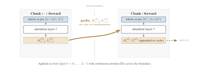

Figure 1 (paper Fig.2): The core mechanism — chunk $t$‘s attention layer treats chunk $t-1$‘s keys/values as an unmodified prefix, and its own output is appended to the cache for chunk $t+1$. Applied identically at every layer $\ell = 0, \dots, L-1$, with position IDs continuing across the chunk boundary (not reset).

The picture above is deceptively simple, and that’s the point. There is no gate, no compression module, no learned routing — the “mechanism” is just: don’t throw away the KV cache between chunks, and don’t reset positions. Everything else is standard transformer inference.

3. Data flow across the whole sequence

flowchart TD
    X0["chunk x_0 (tokens 0..C)"] --> P0["forward pass F_theta"]
    P0 --> KV0["(K^0, V^0)"]
    KV0 --> P1["forward pass F_theta on x_1, prefixed by (K^0,V^0)"]
    X1["chunk x_1 (tokens C..2C)"] --> P1
    P1 --> KV1["(K^1, V^1)  [accumulated]"]
    KV1 --> P2["forward pass on x_2, prefixed by (K^1,V^1)"]
    X2["chunk x_2"] --> P2
    P2 --> KVdots["... accumulates through chunk N-1"]

Figure 2 (self-drawn): The whole sequence processed as foldl(F_theta, (∅,∅), [x_0, x_1, ..., x_{N-1}]) — each step’s output cache becomes the next step’s input prefix, exactly mirroring a functional left fold.

4. Formalizing the recurrence

4.1 The recurrence equation

Let $(\mathcal{K}^{(t)}, \mathcal{V}^{(t)})$ denote the accumulated KV cache (across all layers, though the paper writes it per-layer with superscript $\ell$) after processing chunk $t$. Then:

$$(\mathcal{K}^{(t)}, \mathcal{V}^{(t)}) = \mathcal{F}_\theta\left((\mathcal{K}^{(t-1)}, \mathcal{V}^{(t-1)}), \mathbf{x}_t\right) \tag{2}$$

where $\mathcal{F}_\theta$ is just the ordinary transformer forward function with fixed parameters $\theta$, applied to the current chunk $\mathbf{x}_t$ conditioned on the previous cache as prefix. Unrolling this over the whole sequence gives exactly a left fold:

$$(\mathcal{K}^{(N-1)}, \mathcal{V}^{(N-1)}) = \texttt{foldl}\big(\mathcal{F}_\theta,\ (\emptyset, \emptyset),\ [\mathbf{x}_0, \mathbf{x}_1, \dots, \mathbf{x}_{N-1}]\big) \tag{3}$$

Derivation / intuition. Compare this to what a single full-attention forward pass computes. In full attention, token $i$ in chunk $t$ attends to every token $0, \dots, i-1$ in one shot, computed jointly. In KV-Fold, token $i$ in chunk $t$ attends to the accumulated cache from chunks $0, \dots, t-1$ (computed in earlier, separate forward passes) plus the tokens within its own chunk (computed jointly, as usual). The mathematical content is identical if and only if two conditions hold: (a) position IDs are continuous across the boundary — i.e., token $i$ in chunk $t$ still thinks it’s at absolute position $tC + i$, not $i$ — so that RoPE rotations line up exactly as they would in the full pass; and (b) the numerics of computing $K, V$ for chunk $t-1$ in isolation exactly equal what they’d be inside a single joint forward pass. Condition (a) is exactly satisfied by construction (the paper is explicit about this). Condition (b) is where the interesting empirical behavior comes from — and it is not trivially true, because attention involves a softmax normalization over the full row of keys seen so far, and computing chunk $t-1$‘s keys “as if it were the only chunk” is not literally identical to computing them “as part of a longer running context” — except that per the KV-Fold construction, keys and values themselves don’t depend on later tokens at all (causal masking already guarantees $K_i, V_i$ depend only on tokens $\le i$), so $K^{(\ell)}_s$ computed in the chunked regime is bit-identical, per layer, to what a single joint pass would produce, as long as attention at that layer conditions on the same prefix. The subtlety, which the paper investigates empirically rather than proving analytically layer-by-layer, is whether small floating-point differences introduced by processing chunks as separate kernel calls (different batching, different accumulation order in matmul) compound across depth.

4.2 Three reference conditions

To measure this precisely, the paper defines three conditions per chunk:

• FULL: next-token NLL under a single full-attention forward pass over the entire $T$-token sequence — the reference ceiling.
• ISOLATED: NLL when each chunk is processed with no prefix at all (each chunk sees zero context from earlier chunks) — the floor, representing what you’d get if you just ran chunks independently with no recurrence.
• KV-FOLD: NLL under the accumulated-cache recurrence described above.

And the two headline metrics:

$$\text{drift}(d) = \text{NLL}_{\text{KV-FOLD}}(d) - \text{NLL}_{\text{FULL}}(d) \tag{4}$$ $$\text{advantage}(d) = \text{NLL}_{\text{ISOLATED}}(d) - \text{NLL}_{\text{KV-FOLD}}(d) \tag{5}$$

where $d$ is the chain depth (chunk index minus one, i.e., how many chunk-to-chunk transitions have occurred). Drift measures “how far from the ideal ceiling are we”, and advantage measures “how much better than doing nothing (isolated chunks) are we”. A method that is both low-drift and high-advantage is doing real, useful work rather than degenerating to either extreme.

5. Algorithm: KV-Fold as pseudocode

Algorithm 1 — KV-Fold chunked forward pass

Input: sequence of tokens x[0..T-1], chunk size C, model F_theta with L layers
Output: final KV cache (K, V) over all layers, and per-chunk logits

1.  N ← ceil(T / C)
2.  K[l] ← empty list for each layer l = 0..L-1   # cache init
3.  V[l] ← empty list for each layer l = 0..L-1
4.  for t = 0 to N-1:
5.      x_t ← x[t*C : min((t+1)*C, T)]             # slice t-th chunk
6.      # position IDs continue from absolute offset t*C — NOT reset to 0
7.      logits_t, (k_t[0..L-1], v_t[0..L-1]) ← F_theta.forward(
8.                x_t,
9.                past_key_values = (K, V),          # prefix, unmodified
10.               position_offset = t * C)
11.     for l = 0 to L-1:
12.         K[l].append(k_t[l])                     # grow cache, no eviction
13.         V[l].append(v_t[l])
14.     yield logits_t
15. return (K, V)

This is, deliberately, not an exotic algorithm — it’s exactly what model.generate(..., past_key_values=past_kv) already does in Hugging Face-style APIs, just called repeatedly over successive chunks rather than once over the whole sequence. The “invention” is entirely in the claim that doing this repeatedly is safe, plus the systematic characterization of when it is and isn’t.

Algorithm 2 — Needle-in-a-haystack retrieval protocol (paper’s evaluation procedure)

Input: document D of T tokens split into N chunks, needle (key, value) pair,
       target chain depth d (chunk index at which to query)
Output: retrieval success (boolean)

1.  Insert sentence "The magic number for [key] is [value]." at chunk position N-1-d
2.  Run Algorithm 1 over all N chunks, retaining final (K, V)
3.  Construct query: "Earlier in the document, what was the magic number
    associated with [key]? Reply with only the number."
4.  logits, _ ← F_theta.forward(query, past_key_values=(K,V), position_offset=T)
5.  answer ← greedy_decode(logits, max_new_tokens=30)
6.  extracted ← extract_first_5digit_number(answer)
7.  return extracted == value

6. Design choice: why continuous position IDs matter (and where they can fail)

The choice. Position IDs for chunk $t$ start at $tC$, not $0$ — i.e., the model is never told “a new sequence has started”; RoPE rotations are applied exactly as they would be in one giant forward pass.

Why it works. RoPE encodes relative position through the rotation angle difference between a query and a key. If chunk $t-1$‘s keys are rotated as if they were at position $[(t-1)C, tC)$ and chunk $t$‘s queries are rotated as if they were at $[tC, (t+1)C)$, the relative angle between any query-key pair is identical to what it would be in a single full pass — that’s the whole trick that makes the cache directly reusable without any transformation (“no copy, no transformation” as the architecture figure states).

The obvious alternative. Reset positions to $0$ at each chunk boundary (treat each chunk as a fresh mini-sequence that happens to have some extra keys visible). This is simpler to implement in some serving stacks, but it breaks RoPE’s relative-position semantics: a key from chunk $t-1$ at “position 0” attended by a query from chunk $t$ at “local position 5” would encode a relative distance of 5, when the true distance in the original sequence is $C + 5$. This corrupts every attention score involving cross-chunk pairs.

Where continuous positions fail. The scheme is only exact within the model’s trained position range. Once $tC$ exceeds the maximum position the model was trained/extrapolated for (its native context window, e.g., 128K for Llama-3.1-8B), you’re now relying on RoPE extrapolation behavior outside training distribution — a well-known source of degradation independent of KV-Fold itself. The paper is explicit that all its experiments keep $T$ within the model’s native window for exactly this reason; it does not test what happens if KV-Fold is pushed past the trained position range (that would conflate “recurrence instability” with “position-extrapolation instability”, two different failure modes).

7. The central empirical result: drift saturates

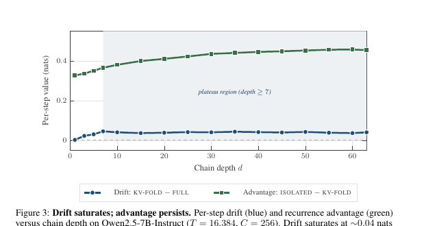
Figure 3 (paper Fig.3): per-step drift (blue) and recurrence advantage (green) versus chain depth on Qwen2.5-7B-Instruct ($T=16{,}384$, $C=256$). Drift rises during the first ~7 transitions to about 0.04 nats, then stays flat through depth 63; advantage stays positive and even grows slightly throughout.

The reported numbers: drift changes by only $-0.0003$ nats between depth 15 and depth 60 — “well within window-to-window noise ($N=42$)” as the paper puts it. In other words, past the initial transient, running the chain deeper costs essentially nothing extra in terms of divergence from full attention. This is the crux of the “stable regime” interpretation: KV-Fold does not behave like an iterated numerical approximation accumulating rounding error linearly (or worse, geometrically) with depth; instead, it looks like the system settles into a nearby fixed point after the first chunk transition and stays there.

Why this matters mechanically. Full attention and KV-Fold compute the same function of the same underlying tokens, conditioned identically at every position — the only difference is how many separate kernel invocations were used to compute the keys/values that get attended to. If this were purely additive floating-point noise, you would expect drift to grow (roughly) with $\sqrt{d}$ or $d$ depending on error accumulation model, not plateau. The plateau instead suggests that whatever discrepancy KV-Fold introduces is a one-time shift in the KV cache distribution at the first boundary, and once the model has “seen” cache states from this new regime, subsequent chunks don’t introduce additional shift — because the model’s attention computation is Lipschitz-ish/robust enough that small perturbations to distant past keys don’t blow up.

8. Design choice: why is drift structural, not numerical?

This is the paper’s second major empirical thrust, and it deserves its own unpacking because it’s the part that turns “we observed a flat line in one experiment” into “here is a claim about why the flat line exists.”

Robustness test 1 — precision. The paper reruns the drift measurement at bf16 vs. fp32 — a $10{,}000\times$ change in per-operation numerical precision (bf16 has ~3 decimal digits of mantissa precision; fp32 has ~7). If drift were caused by floating-point rounding error compounding across chunk boundaries, going to fp32 should shrink it dramatically. Instead, the plateau shrinks by only 2.8%. This is the single strongest piece of evidence that drift is not a numerical artifact.

Robustness test 2 — chunk size. Sweeping chunk size $C$ across an 8× range (128 → 1024) changes the plateau by less than 9%, with no monotonic trend. If drift were an artifact of, say, kernel-level batching differences that scale with chunk granularity, you’d expect a clear trend with $C$. There isn’t one.

Robustness test 3 — architecture. The same qualitative saturation curve (rise then plateau) reproduces across Qwen2.5-7B, Llama-3.1-8B, and OLMoE — three different model families with different attention implementations, head counts, and (in OLMoE’s case) a sparse MoE architecture. The plateau magnitude differs across models (as you’d expect — different models have different sensitivity to distributional shift), but the qualitative shape is consistent.

The alternative explanation the paper is implicitly ruling out. One might worry that “stability” here is really “the model has stopped paying attention to old tokens anyway, so of course drift plateaus — it’s just attention saturation/dilution, not a genuine recurrence property.” The needle-in-a-haystack results (Section 9 below) directly address this: if the model were dilution-saturating and effectively ignoring distant chunks, exact retrieval of a fact planted 511 chunk-transitions back should fail. It doesn’t. So the plateau in drift coexists with preserved content-based addressing to old positions — which is a stronger and more interesting claim than mere saturation.

Where this could still be fragile. All three robustness checks are conducted on PG-19 (long-form book text) with the same measurement protocol (sample fixed windows, greedy/bf16-consistent decoding unless testing precision). None of them test truly adversarial or out-of-distribution chunk boundaries — e.g., a chunk boundary that happens to fall in the middle of a critical dependency (a code block that only makes sense with a variable defined many tokens earlier under unusual syntax, or a legal document with heavy cross-referencing). The paper’s own Discussion section (Section 8) acknowledges a related caveat about quantization robustness that generalizes here: the recurrence “tolerates noise-like perturbations… but is sensitive to systematic information loss.” An out-of-distribution content structure that systematically confuses attention at every chunk boundary is a form of systematic rather than noise-like perturbation, and the paper’s robustness tests don’t rule this out.

9. Long-range retrieval: does the plateau actually preserve information?

Table 1 (paper Table 3): needle-in-a-haystack retrieval on Qwen2.5-7B-Instruct at $T=16{,}384$ ($C=256$, 20 trials/distance).

Distance $d$	FULL	ISOLATED	KV-FOLD	ratio
1	100% (20/20)	0% (0/20)	100% (20/20)	1.00
15	100% (20/20)	0% (0/20)	100% (20/20)	1.00
31	100% (20/20)	0% (0/20)	100% (20/20)	1.00
62	100% (20/20)	0% (0/20)	100% (20/20)	1.00
overall	100% (80/80)	0% (0/80)	100% (80/80)	1.00

This table is doing a lot of work: KV-Fold matches the FULL upper bound exactly, at every tested distance, while ISOLATED (no recurrence at all) fails completely — confirming that the recurrence itself, not some other artifact of chunking, is what preserves the fact.

Multi-needle stress test. A single planted fact is a relatively easy case (models are known to be good at single-needle retrieval even under lossy compression). The paper strengthens this by inserting $K \in \{4, 8\}$ independent (key, value) pairs simultaneously and querying each one separately (Table 2, paper Table 5): 175/176 needles recovered correctly across all configurations (99.4%), with the single miss at $K=4$, a middle-distance position — i.e., not a systematic failure mode, but an isolated miss consistent with ordinary model noise.

Model	$T$	$K$	trials	per-needle	all-correct	ISOLATED
Qwen2.5-7B	16K	2	10	20/20 (100%)	10/10	0/20
Qwen2.5-7B	16K	4	10	39/40 (97.5%)	9/10	0/40
Qwen2.5-7B	16K	8	10	80/80 (100%)	10/10	0/80
Llama-3.1-8B	128K	4	3	12/12 (100%)	3/3	0/12
Llama-3.1-8B	128K	8	3	24/24 (100%)	3/3	0/24
combined			36	175/176 (99.4%)	35/36	0/176

10. Scaling to 128K and the memory/compute cost

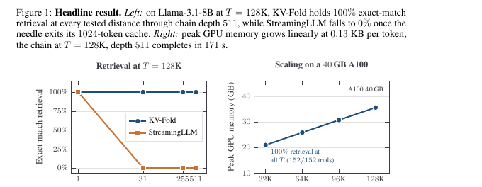
Figure 4 (paper Fig.1): headline results reproduced — left panel shows KV-Fold holding 100% exact-match retrieval at every tested distance through chain depth 511 while StreamingLLM collapses to 0% past distance 1; right panel shows peak GPU memory growing linearly with $T$, reaching 35.6GB at 128K on a 40GB A100.

10.1 Memory scaling derivation

The KV cache at chain depth $t$ stores keys/values for all $tC$ tokens seen so far, across all layers and heads. For a model with $L$ layers, $H_{kv}$ KV-heads, head dimension $d$, and bf16 storage:

$$\text{bytes per token} = L \times H_{kv} \times d \times 2 \ (\text{K and V}) \times 2\ (\text{bf16 bytes}) \tag{6}$$

For Llama-3.1-8B ($L=32$, $H_{kv}=8$, $d=128$):

$$32 \times 8 \times 128 \times 2 \times 2 = 131{,}072 \text{ bytes/token} = 0.128 \text{ KB/token} \tag{7}$$

which matches the paper’s measured $0.13422$ KB/token almost exactly (the small gap is likely additional serving overhead — padding, allocator granularity). At $T=128\text{K}$:

$$128{,}000 \times 0.134 \text{ KB} \approx 17.2 \text{ GB} \tag{8}$$

— matching Table 4’s reported 17.18GB cache size. Peak GPU memory (35.6GB) also includes activations and the model weights themselves (~16GB for an 8B model in bf16), leaving only about 4.4GB headroom on a 40GB card at this operating point — which the paper flags directly as “the operational ceiling.”

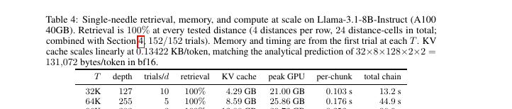
Table 3 (paper Table 4): single-needle retrieval, memory, and compute at scale on Llama-3.1-8B-Instruct (A100 40GB).

$T$	depth	trials/$d$	retrieval	KV cache	peak GPU	per-chunk	total chain
32K	127	10	100%	4.29 GB	21.00 GB	0.103 s	13.2 s
64K	255	5	100%	8.59 GB	25.86 GB	0.176 s	44.9 s
96K	383	3	100%	12.88 GB	30.72 GB	0.252 s	96.9 s
128K	511	3	100%	17.18 GB	35.57 GB	0.335 s	171.3 s

10.2 Compute scaling derivation

At chain depth $t$, attention over the current chunk against the whole accumulated cache costs roughly $O(C \cdot tC \cdot H \cdot L)$ (query length $C$, key length $tC$). Summing over all $N = T/C$ chunks:

$$\text{total compute} \approx \sum_{t=0}^{N-1} O(C \cdot tC \cdot H \cdot L) = O\!\left(\frac{L H C^2 N^2}{2}\right) = O\!\left(\frac{L H T^2}{2}\right) \tag{9}$$

which recovers the same $O(T^2)$ total FLOPs as a single full-attention pass — as it must, since KV-Fold computes an attention pattern equivalent to full causal attention, just spread over multiple kernel calls. The measured per-chunk times (0.103 → 0.176 → 0.252 → 0.335 s for $T=32\text{K} \to 128\text{K}$) grow roughly linearly with the mean cache size the chunk attends against, consistent with this derivation.

Design choice: why does this help at all if total FLOPs are unchanged? The saving is entirely in peak working memory, not total compute. A single full-attention forward at $T=128\text{K}$ requires materializing the $[H, T, T]$ score matrix — roughly 1TB as computed in Eq. (1), infeasible regardless of how much total compute budget you have. KV-Fold’s largest per-chunk score matrix is $[H, C, T]$ — at $C=256$, $H=32$, $T=128\text{K}$, that’s about 2.1GB, comfortably within budget. This is a reorganization of when memory is needed, not a reduction in the amount of work done — closer in spirit to gradient checkpointing (same FLOPs, different memory profile) than to an approximation method.

11. Design choice: comparison against StreamingLLM

Table 4 (paper Table 6): comparison at $T=128\text{K}$, chain depth 511.

Method	NLL	peak GPU	total wall	$d{=}1$	$d{=}31$	$d{=}255$	$d{=}511$
KV-Fold	2.46 ± 0.12	35.6 GB	166 s	3/3	3/3	3/3	2/3*
StreamingLLM	2.66 ± 0.17	16.6 GB	22 s	3/3	0/3	0/3	0/3

*One of three trials at $d=511$ returned no extractable 5-digit answer; combined with the 12/12 result from the earlier single-needle sweep at the same setting, the joint retrieval rate is 14/15.

Why StreamingLLM works the way it does. StreamingLLM keeps a small fixed number of “attention sink” tokens (typically the first few tokens of the sequence, which empirically absorb a disproportionate share of attention mass — a phenomenon documented in the original StreamingLLM paper) plus a bounded sliding window of the most recent tokens (1020 in this comparison, for a 1024-token effective cache). This bounds memory at a constant 0.13GB regardless of $T$ — vastly cheaper than KV-Fold’s linearly-growing cache — and correspondingly the wall-clock is 7.5× faster (22s vs. 166s at this operating point).

The trade-off, stated precisely. The two methods are not competing on the same axis. StreamingLLM optimizes for bounded-memory streaming with acceptable perplexity, where “acceptable” means the model doesn’t need to recall specific facts from arbitrarily far back — a reasonable assumption for open-ended chat or monitoring use cases where only recent context matters. KV-Fold optimizes for exact long-range recall, at the cost of memory that grows (linearly, not compressed) with total context length. Table 4 makes this precise: at every distance beyond the sliding window’s reach (31, 255, 511 chunk-transitions back), StreamingLLM drops to 0% because the needle has literally been evicted from its cache — this is not a soft degradation, it’s a hard architectural ceiling. KV-Fold pays 35.6GB and 166s to avoid that ceiling entirely.

Where KV-Fold could lose this comparison in practice. If your actual workload rarely requires recall beyond a bounded recent window — most conversational or monitoring workloads — StreamingLLM’s 7.5× speedup and near-zero memory footprint is the objectively better engineering choice, and KV-Fold’s guarantee is paying for a capability you don’t need. KV-Fold is the right tool specifically when (a) you need retrieval at arbitrary depth, and (b) you have the memory budget to carry a linearly-growing cache up to your operational ceiling (roughly the model’s native context window, by the paper’s own extrapolation).

12. Robustness to storage-level perturbation (quantization)

The Discussion section reports a further robustness check: quantizing the KV cache with a per-step round-trip (bf16 → int$N$ → bf16) on Llama-3.1-8B at $T=128\text{K}$, chain depth 511. At int8, retrieval holds at 13/14 trials (93%, with the single miss returning no extractable answer, not a wrong answer). At int4, retrieval drops to 24/33 (73%), “down from 100% at moderate depths” per the paper. The paper’s own framing is instructive: “the recurrence tolerates noise-like perturbations… but is sensitive to systematic information loss (decay or eviction remove specific positions entirely).” Quantization noise is roughly uniform and non-targeted (it doesn’t specifically destroy the needle’s tokens), whereas eviction (as in streaming methods) targets old positions systematically and unconditionally. This is a clean, testable distinction, and it’s consistent with everything else the paper shows: KV-Fold’s guarantee is about preserving addressability of specific positions, and any perturbation that specifically and systematically removes position-addressable information (not just adds noise to it) will break that guarantee.

13. Practical deployment notes (beyond what the paper states)

A few operational details worth knowing if you actually want to wire this up:

• Cache placement across GPUs. At 17GB at 128K, the cache won’t fit comfortably alongside model weights on smaller GPUs. Multi-GPU deployments either pin the whole cache to a single device (paying cross-device attention overhead) or shard it PagedAttention-style; KV-Fold composes naturally with chunked serving infrastructure like vLLM, but the serving scheduler must be configured to not compress or evict past chunks, since that would silently reintroduce the streaming trade-off KV-Fold is designed to avoid.
• Prefill vs. decoding. What the paper calls “chunked recurrence” is essentially a controlled, staged prefill. Once the last chunk is processed and the cache is built, ordinary token-by-token decoding proceeds unchanged — it simply operates on a cache that happens to have been built incrementally rather than in one shot.
• Checkpointing for interactivity. A useful pattern not discussed in the paper: checkpoint the accumulated cache every $k$ chunks so an interactive session can rewind to an earlier point without re-prefilling the entire document from scratch.
• Monitoring in production. The paper demonstrates the plateau extends to depth 511 under controlled conditions (PG-19 text, specific models). In a production deployment with more heterogeneous content, I would still monitor per-chunk NLL online to detect cases where the plateau “lifts off” unexpectedly — for example, highly out-of-distribution domains, code with unusual syntax at chunk boundaries, or adversarial inputs.

14. Reproducing the numbers: a worked toy calculation

To build intuition for Eq. (9)‘s compute scaling, consider a toy setting with $C=2$, $T=8$ (so $N=4$ chunks), a single layer ($L=1$), single head ($H=1$). Per-chunk attention cost (ignoring constants) is $C \times (\text{cache size at that step})$:

• Chunk 0: cache size 0 (nothing accumulated yet) → cost $\approx 2 \times 0 = 0$ (chunk still attends within itself, so really $C \times C = 4$, but cross-chunk term is 0)
• Chunk 1: cache size 2 → cross-chunk cost $2 \times 2 = 4$
• Chunk 2: cache size 4 → cross-chunk cost $2 \times 4 = 8$
• Chunk 3: cache size 6 → cross-chunk cost $2 \times 6 = 12$

Total cross-chunk cost: $0 + 4 + 8 + 12 = 24$. Compare to full attention over $T=8$: cost is roughly $T^2/2 = 32$ (upper-triangular causal mask). These are the same order of magnitude ($O(T^2)$), confirming Eq. (9)‘s claim that KV-Fold doesn’t save total FLOPs — it just spreads them out so that no single kernel call needs the full $T \times T$ matrix in memory at once.

15. Notation reference

Symbol	Meaning
$T$	Total sequence length in tokens
$C$	Chunk size in tokens
$N$	Number of chunks, $N = T/C$
$L$	Number of transformer layers
$H$	Number of query heads
$H_{kv}$	Number of KV heads (GQA models may have $H_{kv} < H$)
$d$	Head dimension
$\mathcal{K}^{(t)}, \mathcal{V}^{(t)}$	Accumulated KV cache after processing chunk $t$
$\mathcal{F}_\theta$	Standard transformer forward function, fixed parameters $\theta$
FULL	Reference: single full-attention pass over all $T$ tokens
ISOLATED	Reference: each chunk processed with no prefix
KV-FOLD	The method: chunk $t$ attends to accumulated cache from chunks $0..t{-}1$
drift($d$)	$\text{NLL}_{\text{KV-FOLD}}(d) - \text{NLL}_{\text{FULL}}(d)$
advantage($d$)	$\text{NLL}_{\text{ISOLATED}}(d) - \text{NLL}_{\text{KV-FOLD}}(d)$
plateau	The flat region of drift after the initial transient

16. Limitations and boundary conditions

• Position range dependence. All experiments stay within each model’s native trained context window (Llama-3.1-8B’s 128K). The paper does not test what happens when $T$ exceeds this range, which would require composing with position-extrapolation methods (YaRN, Positional Interpolation, LongRoPE) — explicitly flagged by the authors as future work, not a solved problem.
• Memory does not actually shrink. KV-Fold’s cache at depth $N$ stores exactly the same information a full forward over $NC$ tokens would need. The benefit is entirely operational (spreading peak memory over time), not a reduction in total memory or compute footprint. If your hardware genuinely cannot hold the full linear-growth cache, KV-Fold does not help you — you’re back to needing a compression method.
• Text domain of the robustness sweeps. The precision/chunk-size/architecture robustness experiments (Section 3.1 of the paper) all use PG-19 book text. Whether the same structural (non-numerical) drift behavior holds for very different content distributions — source code, structured tabular data, multi-turn dialogue with abrupt topic shifts — is untested.
• Model scale. Experiments use 7-8B-parameter models. Whether the plateau phenomenon (and its magnitude) holds similarly for much larger or much smaller models, or for models with substantially different attention variants (e.g., linear attention hybrids, heavily sparse attention patterns), is unverified by this paper.
• Quantization degrades gracefully but does degrade. The int4 result (73% retrieval, down from 100%) shows the “noise-like perturbations are fine” claim has real limits — it is not free lunch to combine KV-Fold with aggressive cache quantization for memory savings.

17. Critical analysis

Weaknesses and flaws specific to this paper. The central “stability” claim rests almost entirely on two model families’ worth of PG-19 experiments (Qwen2.5-7B, Llama-3.1-8B, plus a smaller OLMoE check) and a synthetic needle-in-a-haystack task. Needle-in-a-haystack is a well-known “necessary but not sufficient” proxy for genuine long-context understanding — it tests literal string/fact recall, not the kind of reasoning over distant context (e.g., “does what happened in chapter 2 change how I should interpret chapter 40?”) that real long-document use cases often actually need. A model could pass every needle test in this paper while still failing to correctly integrate distant context into a downstream reasoning chain, because retrieval and integration are different capabilities. The paper does not test any reasoning-over-long-context benchmark (e.g., long-document QA requiring multi-hop synthesis, or code understanding requiring cross-file dependency tracking), so the practical scope of the “stability” claim is narrower than the framing (“frozen pretrained transformers already contain the ingredients for long-context reasoning” — from the conclusion) suggests. “Recall” and “reasoning” are being used somewhat interchangeably in the paper’s rhetoric where the evidence only supports the former.

Limitations the authors understate or omit. The paper is admirably candid about memory not shrinking and about the position-range boundary, but it is less forthcoming about the wall-clock cost relative to other long-context methods that also preserve exact recall (not just streaming baselines, which trade away recall by design). There’s no comparison against, e.g., a well-tuned KV-cache eviction method that uses attention-score-based importance heuristics (H2O-style) rather than naive sliding windows — such methods try to keep the important tokens rather than just the recent ones, and might achieve much better retrieval than plain StreamingLLM while still using far less memory than KV-Fold. Without that comparison, it’s hard to know whether KV-Fold’s “exact recall” advantage over streaming specifically generalizes to an advantage over the broader, more sophisticated compression literature, or whether it’s specifically beating a strawman-ish baseline (uniform sliding window with no importance weighting) that the field has already moved past in more recent work.

Concrete, specific improvement suggestions.

1. Add a genuine long-document reasoning benchmark (e.g., a subset of LongBench or RULER’s multi-hop tasks, or a synthetic “chapter 2 changes interpretation of chapter 40” task) to test whether the preserved information is actually usable downstream, not just retrievable verbatim.
2. Compare against at least one importance-weighted KV compression method (H2O, SnapKV, or similar), not only against a plain sliding-window baseline, to establish where KV-Fold sits on the real Pareto frontier of memory vs. recall rather than only against the cheapest possible comparison point.
3. Test a genuinely adversarial chunk-boundary condition — e.g., deliberately split a chunk boundary in the middle of a syntactically load-bearing construct (an unclosed bracket, an incomplete sentence with a pronoun whose antecedent is in the next chunk) — to stress-test whether the “structural, not numerical” drift claim holds when chunk boundaries are chosen adversarially rather than at fixed, content-agnostic intervals.
4. Report variance/confidence intervals more consistently. Several of the headline numbers (e.g., Table 4’s single-trial-per-$T$ memory/timing figures) are reported from “the first trial” rather than averaged, which makes it hard to assess measurement noise in the systems-level numbers (memory, wall-clock) the way the paper carefully does for the NLL-based drift numbers.
5. Push the position-range boundary explicitly, even briefly, by combining KV-Fold with one position-extrapolation method (YaRN is explicitly mentioned as future work) and reporting whether the plateau behavior survives — this is the single most obvious “next experiment” implied by the paper’s own limitations discussion, and its absence leaves the “how far can this actually scale” question unresolved even in the paper’s own terms.

18. Reproducibility notes

• Code is not linked in the version reviewed (no GitHub URL found in the arXiv v1 PDF); the method itself is simple enough (Algorithm 1 above) to reimplement directly against any Hugging Face-compatible past_key_values API.
• Models used: Qwen2.5-7B-Instruct, Llama-3.1-8B-Instruct, and OLMoE (exact variant not fully specified beyond “OLMoE” in the cross-architecture table).
• Evaluation text: PG-19 validation split, fixed random seed, windows starting 200 tokens into a document.
• Hardware: single 40GB A100 for all reported memory/timing figures.
• Precision: bf16 by default; fp32 and int8/int4 variants used specifically for the robustness ablations described in Sections 8 and 12 of this review.

19. A practitioner’s decision framework: when should you actually reach for KV-Fold?

Given everything above, it’s worth condensing the trade-off into something directly actionable, because the paper’s own framing (“frozen transformers already contain the ingredients for long-context reasoning”) can make it tempting to treat KV-Fold as a universal drop-in upgrade. It is not — it is a specific point on a specific trade-off curve, and the decision of whether to use it should be driven by the shape of your actual workload, not by the elegance of the foldl framing.

Decision variable 1: does your task require exact retrieval at unbounded distance, or just “reasonably recent” context? If your application is a customer support chatbot where only the last few turns of conversation matter, or a monitoring system that only needs to reason about the last hour of logs, you almost certainly do not need KV-Fold’s guarantee — a bounded sliding window (StreamingLLM-style) will give you 7.5x faster wall-clock and a fraction of the memory, at the cost of a capability (arbitrary-depth recall) you were never going to use anyway. If your application is repository-scale code assistance (a function defined at the top of a 50K-line file, referenced at the bottom), longitudinal medical record review, or legal document analysis with heavy cross-referencing, then unbounded recall is not a nice-to-have, it is the whole point, and KV-Fold’s trade-off becomes directly relevant.

Decision variable 2: what is your actual memory budget relative to your typical context length? KV-Fold’s cache grows at a fixed, predictable rate (Eq. 6-8: ~0.13KB/token for an 8B-class model). If you can compute, in advance, that your 95th-percentile context length times this per-token cost still leaves comfortable headroom on your serving hardware, KV-Fold is operationally straightforward to adopt. If your worst-case context length would push you past your GPU’s memory ceiling, KV-Fold does not solve your problem — you are back to needing an eviction or compression strategy, and the honest comparison is not KV-Fold vs. StreamingLLM but KV-Fold vs. an importance-weighted compression method (Section 17’s suggestion 2), which this paper does not provide.

Decision variable 3: is your task retrieval-shaped or reasoning-shaped? As argued in Section 17, needle-in-a-haystack tests literal fact recall, not multi-hop synthesis across distant context. If your task genuinely only requires “find and repeat back a specific fact from earlier” (log lookup, ID lookup, a specific line of code), the evidence in this paper directly supports using KV-Fold. If your task requires integrating and reasoning over information distributed across a long document (e.g., “does the constraint introduced in section 2 conflict with the assumption made in section 40”), this paper’s evidence base does not directly speak to whether KV-Fold helps, because it was never tested on that kind of task.

A simple heuristic summary:

Situation	Recommended approach
Bounded recent context is enough, latency-sensitive	StreamingLLM / sliding window
Need exact recall at arbitrary depth, memory budget comfortably covers worst-case $T$	KV-Fold
Need exact recall at arbitrary depth, memory budget is tight	Importance-weighted KV compression (untested against KV-Fold in this paper — proceed with your own benchmarking)
Need multi-hop reasoning over distant context, not just recall	Untested by this paper either way; benchmark directly on your task
Context length routinely exceeds the model’s native trained position range	Compose with a position-extrapolation method first (YaRN / LongRoPE); this paper does not test that combination

This framework is not in the paper itself — it’s my own synthesis of where the paper’s evidence base actually supports a recommendation versus where it is silent, and I’d treat any of these recommendations as a starting hypothesis to validate on your own workload rather than a guarantee.

20. Conclusion

KV-Fold’s contribution is not a new architecture or a new training recipe — it’s an empirical claim about an existing capability of frozen transformers, characterized carefully enough to be useful. Treating the KV cache as a left-fold accumulator across chunks turns an intractable single forward pass into a sequence of tractable ones, at the cost of linear (not compressed) memory growth, and the paper’s central evidence — the drift plateau that survives massive precision changes, chunk-size sweeps, and architecture changes — is a genuinely interesting empirical finding about how robust transformer attention is to this kind of chunked reorganization. The needle-in-a-haystack results back this up with task-level evidence rather than resting purely on aggregate NLL. Where the paper is honest about its limits (memory doesn’t shrink, position range is bounded by training, quantization tolerance has a ceiling), it earns trust; where it leans on the rhetorical framing of “long-context reasoning” while only demonstrating exact recall, readers should hold the claim to the narrower, better-supported version: KV-Fold reliably preserves retrievable information across long chains, on the content distributions tested so far.