July 25, 2026 EN #LLM Agent #Multi-Agent Systems #Reasoning

When Does Adding More Agents Actually Help? An Information-Bottleneck Answer

Review date: 2026-07-25 Review author: Zhongzhu Zhou Paper reviewed: When Do Multi-Agent Systems Help? An Information Bottleneck Perspective Paper authors: Wendi Yu, Lianhao Zhou, Xiangjue Dong, Sai Sudarshan Barath, Declan Staunton, Byung-Jun Yoon, Xiaoning Qian, James Caverlee, Shuiwang Ji (Texas A&M University; Brookhaven National Laboratory) arXiv: 2607.16133 Status: Preprint, submitted 17 July 2026

Short Answer

If you’ve ever wired up a multi-agent LLM pipeline and watched it underperform a single well-prompted agent, this paper explains exactly why, with a formal mechanism rather than a shrug. The authors’ core observation is deceptively simple: a single-agent system (SAS) keeps one growing shared context across the whole task, while a multi-agent system (MAS) splits the task across isolated workers that only talk to each other through short “relay” messages. They first prove that if those relay messages could carry unlimited information, a MAS could always simulate a SAS exactly — so any real advantage or disadvantage of MAS must come from the fact that relays are bandwidth-limited and therefore lossy. They then model each relay as an information bottleneck: it should throw away context that is irrelevant to the downstream worker’s task while keeping everything relevant. This yields a clean decomposition of “MAS gain” into two competing terms — the benefit of removing noisy upstream context, and the cost of losing information the next worker actually needed — with the balance point controlled by an effective parameter β that increases with the downstream model’s capability. Across 18 controlled experiments spanning five agentic benchmarks (ALFWorld, WebShop, WorkBench, WideSearch, TravelPlanner) and three model scales (Qwen2.5-7B, GPT-4o-mini, Qwen3.5-27B), the predicted pattern holds up: MAS reliably wins when the task’s relays can be short and still sufficient (context reduction dominates), and MAS gains shrink or even flip negative as either the task demands richer cross-step context or the base model becomes strong enough to exploit that context itself. This turns “should I use multi-agent or single-agent for this task?” from a matter of taste into a question you can reason about structurally, before you’ve spent a single API dollar on an ablation.

Key Takeaways

The paper’s headline theoretical result, Proposition 3.1, shows that under unbounded relay bandwidth, a MAS can always exactly reproduce any SAS’s output — meaning the entire empirical debate about “does splitting into multiple agents help” is really a debate about bounded-bandwidth relay compression, not about decomposition itself.
Theorem 4.1 decomposes local “MAS gain” at any single relay interface into two competing, named quantities: upstream context reduction $H(M_i \mid m_i)$ (a benefit) and relay information loss $\Delta_i(m_i)$ weighted by capability $\beta$ (a cost) — MAS wins locally exactly when $H(M_i \mid m_i) > \beta \Delta_i(m_i)$ .
The capability-dependent $\beta$ is the paper’s most practically useful idea: stronger downstream models are hurt more by relay compression (because they could have used the full context productively) and helped less by noise removal (because they’re already good at ignoring irrelevant context), so the same MAS design that helps a 7B model can actively hurt a 27B model on the same task.
A carefully designed three-way controlled comparison (SAS vs. SAS-contextflow vs. MAS) isolates why MAS helps: SAS-contextflow uses the identical planner-induced sub-task decomposition as MAS but keeps one shared context, so any residual gap between SAS-contextflow and MAS is attributable purely to relay-induced context isolation, not to task decomposition.
The empirical results split cleanly along the paper’s own predicted relay-complexity axis $\delta$ : benchmarks with compact sufficient relays (ALFWorld, WideSearch, TravelPlanner-CS, all $\delta \approx 0$ ) show MAS beating SAS-contextflow consistently across all three models, while benchmarks needing detailed cross-step evidence (WorkBench, $\delta \gg 0$ ) show MAS losing to SAS-contextflow at every model scale.
A causal ablation (Table 4 of the paper) directly manipulates relay sufficiency by deliberately deleting downstream-needed fields from the relay message (e.g., stripping price and navigation history from a WebShop relay) and shows performance drops monotonically as designed information loss increases — this is the paper’s strongest evidence that $\Delta_i(m_i)$ is a real causal lever, not just a descriptive post-hoc quantity.

Prerequisites: What You Need to Know First

This paper sits at the intersection of three areas: LLM-based multi-agent systems, information theory (specifically the information bottleneck framework), and empirical agent benchmarking. To follow the derivations without hand-waving, you need five pieces of background, which I build up one at a time below: what an LLM agent’s “context” actually is and how it accumulates, what distinguishes a single-agent from a multi-agent architecture at the level of information flow (not just the number of API calls), what mutual information and conditional mutual information mean and how to read expressions like $I(X;Y\mid Z)$ , what the classical information bottleneck principle is trying to optimize, and what a Markov relation $X \leftrightarrow Y \leftrightarrow Z$ asserts about a system.

What “Context” Means for an LLM Agent

When an LLM is used as an autonomous agent — solving a multi-step task like navigating a simulated household (ALFWorld) or completing a purchase on a mock e-commerce site (WebShop) — it doesn’t see the whole task at once. It operates in a loop: observe the current state of the world in text form, decide on an action, receive a new observation reflecting the consequence of that action, and repeat. The context at any point in time is the accumulated transcript of everything the agent has seen and done so far: prior observations, its own intermediate reasoning (“thoughts”), and the actions it took. This context is what actually gets fed back into the LLM at every step — it is functionally the agent’s entire “memory” of the episode, since the underlying LLM itself has no persistent state between calls. A key practical fact worth internalizing: as an episode gets longer, this context grows, and everything in it competes for the LLM’s limited attention and context window. This is the seed of the entire paper’s argument — a shared, ever-growing context is exactly what a single-agent system relies on, and exactly what a multi-agent system deliberately gives up in exchange for isolation.

Single-Agent vs. Multi-Agent: The Real Structural Difference

The intuitive story about multi-agent systems (MAS) is “specialization” — a planner agent, a coder agent, a critic agent, each good at one thing. But the paper argues the deeper structural difference is about information flow, not division of labor. A single-agent system (SAS) is one agent that carries one shared, monotonically growing context through the entire task: every subtask’s outcome, every intermediate observation, stays visible to every later step. A multi-agent system (MAS), by contrast, assigns different phases of the task to different “workers,” each of which starts with a fresh, isolated context — it only receives its own sub-instruction plus a short relay message summarizing whatever the previous worker decided was worth passing forward. Crucially, this means a MAS worker cannot see the raw history that produced the relay message — only the compressed summary. This is the structural fact the whole paper is built on: MAS isn’t “SAS plus specialization,” it’s “SAS with the shared context replaced by a lossy, bottlenecked communication channel between isolated workers.”

Mutual Information and Conditional Mutual Information

The paper’s formal machinery is built entirely out of mutual information, $I(X;Y)$ , which measures (in bits, or nats) how much knowing the value of random variable $X$ reduces your uncertainty about random variable $Y$ . Formally, $I(X;Y) = H(Y) - H(Y\mid X)$ , where $H(\cdot)$ is Shannon entropy (a measure of uncertainty) and $H(Y\mid X)$ is the conditional entropy — the remaining uncertainty about $Y$ once $X$ is known. If $X$ and $Y$ are completely independent, $I(X;Y) = 0$ : knowing $X$ tells you nothing new about $Y$ . If $Y$ is a deterministic function of $X$ , $I(X;Y) = H(Y)$ : knowing $X$ tells you everything about $Y$ . The paper also uses conditional mutual information, $I(X;Y\mid Z)$ , which measures how much $X$ tells you about $Y$ after already conditioning on (i.e., given) $Z$ . This is the quantity that appears throughout Section 4: expressions like $I(m_i; Y_{i+1} \mid X_{i+1})$ ask “how much does the relay message $m_i$ tell us about the downstream target $Y_{i+1}$ , once we already know the downstream sub-instruction $X_{i+1}$ ?” — i.e., the additional, non-redundant predictive value of the relay, above and beyond what the sub-instruction itself already implies.

The Information Bottleneck Principle

The information bottleneck (IB) framework, originally due to Tishby, Pereira, and Bialek, formalizes a very general compression problem: given an input $X$ and a target variable $Y$ you care about predicting, find a compressed representation $T$ of $X$ that keeps as much information about $Y$ as possible while discarding as much irrelevant information about $X$ as possible. This is stated as an optimization problem,

\min_{p(T\mid X)} \; I(X;T) - \beta I(T;Y),

where $I(X;T)$ (how much of $X$ survives into $T$ ) is being minimized — you want a small, compressed $T$ — while $I(T;Y)$ (how predictive $T$ still is of $Y$ ) is being maximized, with a Lagrange multiplier $\beta > 0$ controlling the trade-off between the two competing goals. When $\beta$ is small, the objective favors aggressive compression even if it costs some predictive power; when $\beta$ is large, the objective favors preserving predictive information even at the cost of a less-compressed representation. This exact template — minimize how much upstream information survives, while maximizing how much of it is useful for a downstream target — is what the paper transplants directly onto the design of a MAS relay message: the relay $m_i$ plays the role of the compressed representation $T$ , the worker’s full context $M_i$ plays the role of the input $X$ , and the next worker’s target $Y_{i+1}$ plays the role of the prediction target.

Markov Relations: What $X \leftrightarrow Y \leftrightarrow Z$ Means

A Markov chain (or Markov relation) $X \leftrightarrow Y \leftrightarrow Z$ asserts that $X$ and $Z$ are conditionally independent given $Y$ : once you know $Y$ , learning $X$ gives you no additional information about $Z$ , and vice versa. Formally, $p(z \mid x, y) = p(z \mid y)$ . Intuitively, $Y$ is a “sufficient intermediary” between $X$ and $Z$ — all of the influence $X$ has on $Z$ must flow through $Y$ . This becomes important in Section 4.1 of the paper, which establishes the Markov relation $m_i \leftrightarrow M_i \leftrightarrow Y_{i+1} \mid X_{i+1}$ : the relay $m_i$ is derived from (compressed from) the full context $M_i$ , and cannot contain information about the downstream target $Y_{i+1}$ that isn’t already present in $M_i$ itself. This is what licenses treating the relay-design problem as a bottleneck problem in the first place — the relay can only ever be as informative as its source, never more.

Notation Reference Table

Because Section 4’s derivations introduce a number of subscripted symbols in quick succession, here is a single table to refer back to while reading the method section below.

Symbol	Meaning
$X$	a full task instance
$X_1, \ldots, X_n$	planner-induced sub-instances assigned to workers $1, \ldots, n$
$Y_i$	the worker-specific target variable for sub-instance $X_i$
$M_i$	worker $i$ ‘s full accumulated context
$m_i$	the relay message worker $i$ sends forward, $m_i = \text{Agg}_i(M_i)$
$B_{\text{sys}}$	inter-worker relay bandwidth, $H(m_i) \le B_{\text{sys}}$
$H(\cdot)$	Shannon entropy
$I(\cdot;\cdot)$	mutual information
$I(\cdot;\cdot\mid\cdot)$	conditional mutual information
$\beta$	IB trade-off weight, interpreted as downstream model capability
$\Delta_i(m_i)$	relay information loss at interface $i$ (Definition 4.1)
$L_i^{\text{MAS}}, L_i^{\text{SAS}}$	the MAS/SAS local IB objective values
$G_i^{\text{MAS}}$	local MAS gain, $L_i^{\text{SAS}} - L_i^{\text{MAS}}$
$\delta$	estimated relay complexity of a benchmark (minimum sufficient relay description length)

The Method: Formalizing MAS as Bounded-Bandwidth Relay Compression

Setting Up the Formal Objects

The paper first defines a common abstraction, a basic agent, that both SAS and MAS are built from: an agent is a tuple $\langle \mathcal{T}, \mathcal{M}, \pi^T, \pi^A, \text{Agg}\rangle$ , where $\mathcal{T}$ is a “thought” space (intermediate natural-language reasoning), $\mathcal{M}$ is the context/memory space, $\pi^T$ and $\pi^A$ are policies that produce thoughts and actions respectively given the current context, and $\text{Agg}$ is an aggregation function that produces the final output from the terminal context. Given a task instance $X$ and initial observation $o_0$ , the agent’s context evolves as $M_{t+1} = M_t \oplus (\tau_t, a_t, o_t)$ — at every step, the current thought, action, and resulting observation get appended to the running context, exactly mirroring the “growing transcript” intuition from the prerequisites section above.

A single-agent system (SAS) is simply one basic agent that runs this loop over the whole task, producing one continuous context $M_{\text{SAS}}$ and a final output $y_{\text{SAS}} = \text{Agg}(M_T)$ .

A multi-agent system (MAS) introduces a planner that first splits the task instance $X$ into an ordered sequence of sub-instances $X_1, \ldots, X_n$ , each inducing a worker-specific target variable $Y_i$ (the task-relevant thing worker $i$ is supposed to figure out or produce). Each worker $i$ is a separate basic agent operating only on $X_i$ ; when worker $i$ finishes, it produces a relay message $m_i = \text{Agg}_i(M_i)$ — a compressed summary of its own full context $M_i$ — which gets handed to worker $i+1$ . Worker $i+1$ ‘s initial context is then $M_0^{(i+1)} = (X_{i+1}, o_0^{(i+1)}) \oplus m_i$ : its own sub-instruction plus whatever the previous worker chose to pass along, but crucially not worker $i$ ‘s full context $M_i$ . A system-level aggregator combines all workers’ terminal contexts into the final MAS output.

The single most important structural fact buried in these definitions is this: worker $i+1$ literally cannot see $M_i$ . It only ever sees $m_i$ . Whatever worker $i$ forgot to include in the relay message is permanently lost to every downstream worker — there is no way to “go back and check” the original context. This is the concrete mechanical reason a bounded relay can hurt performance, and it’s worth holding onto as intuition for everything that follows.

Step-by-Step: The Infinite-Bandwidth MAS-SAS Equivalence Proof

Before getting to the bottleneck formulation, the paper proves a foundational sanity-check result, Proposition 3.1: as relay bandwidth $B_{\text{sys}} \to \infty$ , for any SAS there exists a MAS that produces exactly the same output. This matters because it establishes that MAS’s structural differences (planning + relay communication) are not inherently limiting — any performance gap must come from the bandwidth constraint, not from having multiple workers per se. The construction, spelled out as a numbered proof in Appendix A.1 of the paper, works as follows. I unpack it as an explicit algorithm:

Algorithm 1: Constructing a MAS that simulates a given SAS exactly (unbounded relay bandwidth)

Input: A SAS with context trajectory $M_0, M_1, \ldots, M_T$ and final output $y_{\text{SAS}} = \text{Agg}(M_T)$ , and an arbitrary time partition $0 = T_0 < T_1 < \cdots < T_n = T$ .
Planner assignment: Set $X_1 = X$ (the whole task) and $X_i = \emptyset$ for every $i \ge 2$ (all later sub-instances are empty — this construction doesn’t actually decompose the task at all, it just re-labels time intervals as “workers”).
Policy reuse: Give every worker $i$ the same thought and action policies $(\pi^T, \pi^A)$ as the original SAS. Worker $i$ is responsible for reproducing exactly the SAS’s own updates from time $T_{i-1}$ to $T_i$ .
Identity relay: Set the aggregator $\text{Agg}_i$ to be the identity map, so the relay handed forward is the worker’s entire terminal context: $m_i = M^{(i)}_{T_i}$ (no compression at all).
Bandwidth check: Because the SAS context has finite entropy at every step (an assumption), each relay $m_i$ also has finite entropy. So for any $B_{\text{sys}} \ge \max_i H(M^{(i)}_{T_i})$ , every relay satisfies $H(m_i) \le B_{\text{sys}}$ — the construction becomes feasible in the limit $B_{\text{sys}} \to \infty$ .
Inductive equivalence: By induction on $i$ : worker 1 starts from the same initial state as the SAS ( $M_0^{(1)} = (X, o_0) = M_0$ ) and, using identical policies and the identical task kernels, reproduces the SAS’s trajectory exactly up to $T_1$ , so $M^{(1)}_{T_1} \equiv M_{T_1}$ . For the inductive step, worker $i+1$ receives the full relay $m_i = M^{(i)}_{T_i} \equiv M_{T_i}$ (by the inductive hypothesis) and its initial context becomes information-equivalent to the SAS’s context at that point in time, so it, too, reproduces the SAS exactly up to $T_{i+1}$ .
Conclusion: Taking $i = n$ gives $M^{(n)}_{T_n} \equiv M_T$ , so the MAS’s final aggregated output equals $y_{\text{SAS}}$ exactly.

The takeaway from this construction is almost anticlimactic by design: if you’re allowed to pass the entire upstream context forward as the “relay message,” a MAS is just a SAS wearing a disguise. Nothing interesting happens — no gain, no loss — until you’re forced to actually compress $m_i$ down to something smaller than $M_i$ . That’s exactly the regime real deployed systems operate in, since LLM context windows and communication budgets are always finite in practice, and it’s exactly the regime the rest of the paper studies.

Formalizing Relay Design as an Information Bottleneck

Given that bounded relay bandwidth is where all the interesting behavior lives, Section 4 sets up the relay-design problem explicitly as an IB objective. First, the Markov relation from the prerequisites section is established formally (proved in Appendix A.2 by noting that the relay $m_i = \text{Agg}_i(M_i)$ ‘s randomness, if any, is independent of $Y_{i+1}$ given $M_i$ and $X_{i+1}$ ):

m_i \leftrightarrow M_i \leftrightarrow Y_{i+1} \mid X_{i+1}. \tag{1}

This licenses writing the relay-design objective in the standard IB form:

\min_{p(m_i \mid M_i)} \; I(M_i; m_i) - \beta \, I(m_i; Y_{i+1} \mid X_{i+1}), \tag{2}

where the first term measures how much of the upstream context “survives” into the relay (to be minimized — a good relay should be short and free of irrelevant detail), and the second term measures how much downstream-relevant information about $Y_{i+1}$ the relay preserves given the next sub-instruction $X_{i+1}$ (to be maximized — a good relay should still let the next worker do its job). $\beta$ is, as before, the trade-off weight, but the paper gives it a very concrete practical interpretation here: $\beta$ represents the downstream LLM’s capability. A weaker model is more easily confused by noisy, irrelevant leftover context, so it implicitly “prefers” a small $\beta$ (favoring aggressive compression); a stronger model can productively use rich context and therefore implicitly “prefers” a large $\beta$ (favoring information preservation over compression). This single design choice — reframing an abstract Lagrange multiplier as “how good is the model reading this relay” — is what turns an information-theoretic curiosity into a testable, falsifiable empirical prediction, which is exactly what the experiments in the paper go on to test.

Deriving the SAS-as-No-Compression Special Case

An elegant consistency check the paper performs: what happens if you plug the uncompressed relay, $m_i = M_i$ , into the IB objective? Substituting into Eq. (2):

L^{\text{SAS}}_i(\beta) \triangleq L^{\text{MAS}}_i(m_i = M_i; \beta) = H(M_i) - \beta \, I(M_i; Y_{i+1} \mid X_{i+1}). \tag{3}

Here I(M_i; m_i) collapses to $H(M_i)$ (mutual information between something and an identical copy of itself equals its own entropy), and the second term becomes the maximum possible predictive information the context could ever provide about $Y_{i+1}$ , since nothing has been thrown away. This shows algebraically what was intuitively obvious from Proposition 3.1: SAS is the no-compression point in the space of possible relay designs. MAS, by construction, always corresponds to some compressed point in that same space. This reframing is what lets the paper make an apples-to-apples comparison between SAS and MAS purely as different points along one shared axis — the amount of relay compression — rather than as two unrelated architectures.

Deriving the MAS Gain Decomposition (Theorem 4.1)

This is the paper’s central theoretical contribution, and it’s worth deriving in full rather than just quoting. First, define the relay information loss:

Definition 4.1 (Relay Information Loss). The information loss induced by relay $m_i$ is

\Delta_i(m_i) \triangleq I(M_i; Y_{i+1} \mid X_{i+1}) - I(m_i; Y_{i+1} \mid X_{i+1}). \tag{4}

This is simply “how much downstream-relevant information about $Y_{i+1}$ was available in the full context $M_i$ , minus how much of that information actually survived into the compressed relay $m_i$ .” By the Markov relation in Eq. (1), a compressed $m_i$ can never carry more target-relevant information than the source it was compressed from, so $\Delta_i(m_i) \ge 0$ always. When $\Delta_i(m_i) = 0$ , the relay is called sufficient — it lost nothing the next worker needed. When $\Delta_i(m_i) > 0$ , it’s insufficient, and larger values mean more severe, more damaging compression.

Substituting Definition 4.1 back into the general IB objective (Eq. 2), after rearranging the terms (I is expanding $I(m_i; Y_{i+1}\mid X_{i+1}) = I(M_i; Y_{i+1}\mid X_{i+1}) - \Delta_i(m_i)$ and distributing the $-\beta$ ):

L^{\text{MAS}}_i(m_i; \beta) = I(M_i; m_i) + \beta \Delta_i(m_i) - \beta \, I(M_i; Y_{i+1}\mid X_{i+1}). \tag{5}

The last term doesn’t depend on the relay design at all — it’s a fixed property of the task and decomposition — so it drops out of any comparison between two different relay choices for the same worker interface.

Now define the MAS gain relative to the SAS (no-compression) baseline: $G_i^{\text{MAS}} \triangleq L_i^{\text{SAS}} - L_i^{\text{MAS}}$ (gain is defined as reduction in the loss objective — remember the IB objective is something we want small, so a smaller $L^{\text{MAS}}$ than $L^{\text{SAS}}$ is a genuine improvement). Subtracting Eq. (5) from Eq. (3) and simplifying (the shared $-\beta I(M_i;Y_{i+1}\mid X_{i+1})$ term cancels exactly, and $I(M_i;M_i) = H(M_i)$ while $H(M_i) - I(M_i;m_i) = H(M_i\mid m_i)$ by definition of conditional entropy) gives the paper’s headline result:

Theorem 4.1 (MAS Gain Decomposition).

G_i^{\text{MAS}} = \underbrace{H(M_i \mid m_i)}_{\text{upstream context reduction}} \; - \; \underbrace{\beta \, \Delta_i(m_i)}_{\text{model capability} \times \text{relay information loss}}. \tag{6}

Every symbol here has a concrete, checkable meaning. $H(M_i \mid m_i)$ is the residual uncertainty about the full context once you only know the compressed relay — intuitively, “how much noisy, irrelevant clutter did the relay successfully strip away?” This is the benefit term, and it’s always non-negative (you can’t lose entropy you didn’t have). $\beta \Delta_i(m_i)$ is the capability-weighted cost of whatever downstream-relevant signal got thrown away along with the noise. MAS is locally beneficial at this interface exactly when

G_i^{\text{MAS}} > 0 \iff H(M_i \mid m_i) > \beta \, \Delta_i(m_i). \tag{7}

This single inequality is the entire empirical claim of the paper, compressed into one line: context reduction has to outpace capability-weighted information loss. Because $\beta$ increases with downstream model capability, the same relay design and the same task can sit on either side of this inequality depending purely on which model is reading the relay — which is exactly the “MAS helps weak models, hurts strong models” pattern the experiments go on to confirm.

Why “Design Choice X” Was Made This Way — Discussion

Why frame $\beta$ as capability rather than estimate it directly? The obvious alternative would be to try to estimate $\beta$ empirically for a given model (e.g., by fitting it to observed performance data), turning the framework into a predictive, quantitative tool rather than a qualitative, explanatory one. The paper explicitly declines to do this and instead treats $\beta$ as a monotonically-increasing-with-capability qualitative parameter. This is a real limitation the paper itself flags (see Limitations below): it means Theorem 4.1 explains why a pattern should hold and predicts its direction, but cannot tell you in advance, for a brand-new task and model pair, exactly where the crossover point is. The upside of the qualitative choice is generality — you don’t need a costly calibration procedure per model/task pair to get directional predictions — but the cost is that the framework is explanatory rather than a deployable a-priori sizing tool.

Why use relay information loss $\Delta_i$ rather than simply relay length (number of tokens) as the design lever? A shorter relay isn’t necessarily a worse one, and a longer relay isn’t necessarily a better one — what matters is whether the specific bits that got kept are the ones the downstream worker needs. The paper’s Table 4 ablation makes this distinction concrete and causal: they construct “insufficient” relay variants that are not shorter in some crude sense but are specifically stripped of fields known to be downstream-relevant (e.g., dropping object location from an ALFWorld relay, or dropping price/attributes/navigation history from a WebShop relay), and show performance drops as a direct consequence — establishing that it’s the content, not the length, that drives the trade-off. The obvious alternative (using token count as a cheap proxy for relay quality) would have been much easier to measure automatically, but the paper correctly identifies that token count and information sufficiency are only loosely correlated, and a length-based metric would have missed exactly the causal mechanism they wanted to isolate.

Why decompose the task the same way for SAS-contextflow and MAS, rather than compare MAS against an ordinary, non-decomposed SAS directly? This is arguably the paper’s most important experimental-design choice, and it’s worth pausing on why a naive MAS-vs-SAS comparison would have been scientifically weaker. If you only compare MAS against plain SAS, any observed gain is confounded: it could come from the task decomposition itself (breaking a hard problem into easier sub-problems, independent of any context isolation) or from the relay-based context isolation the paper’s theory is actually about. By introducing SAS-contextflow — a single agent that follows the identical planner-induced sub-task sequence as MAS but keeps one shared, uncompressed context throughout — the paper creates a controlled condition that differs from MAS in exactly one variable: whether the shared context is replaced by lossy relays. Any residual gap between SAS-contextflow and MAS is now cleanly attributable to relay compression, not decomposition. This is the paper’s version of a proper ablation, and Section 6’s separate “Does Planning Structure Alone Explain MAS Gains?” experiment (Table 3 of the paper, using a related SAS-Plan variant) directly confirms that decomposition alone, without context isolation, does not reproduce MAS’s gains — SAS-Plan actually performs consistently worse than plain SAS on ALFWorld across all three models, underscoring that the isolation mechanism, not the sub-task structure, is doing the real work.

Where does this design choice fail? The controlled three-prototype comparison (SAS / SAS-contextflow / MAS) is clean for isolating relay compression as a mechanism, but it necessarily fixes the planner’s decomposition strategy across both SAS-contextflow and MAS. If a different decomposition (different subtask boundaries, different assignment of responsibilities to workers) would have produced a more relay-friendly structure — for instance, redesigning WorkBench’s decomposition so that cross-domain evidence-gathering and write-actions are handled by the same worker rather than split across a relay boundary — the paper’s framework doesn’t tell us how to find that better decomposition; it only diagnoses how good or bad a given decomposition’s relays are. The paper acknowledges a version of this limitation implicitly in its “Implications” discussion, which frames “jointly optimizing the relay encoder with the downstream task” as future work, rather than a solved problem.

A Practical Algorithm: Deciding Whether to Use MAS or SAS for a New Task

While the paper itself doesn’t present this as a numbered algorithm, Theorem 4.1 and the five-benchmark taxonomy together imply a concrete, actionable decision procedure that a practitioner could follow before committing engineering effort to a multi-agent architecture. I make this explicit as pseudocode, since clause-15-style unpacking of “how would I actually use this” is exactly the kind of design-level detail the paper’s theory section leaves implicit.

Algorithm 2: Structural triage for MAS vs. SAS on a new task

Input: A candidate task, a planner-induced sub-task decomposition $X_1, \ldots, X_n$ , and a candidate downstream model with informally known capability tier (weak / medium / strong).
Estimate relay complexity $\delta$ for each worker interface by asking: does the next worker’s target $Y_{i+1}$ require exact, hard-to-summarize evidence from the upstream worker (object IDs, timestamps, running totals, global constraints) or can it be satisfied by a compact, natural-language summary? If the former, assign $\delta \gg 0$ ; if the latter, $\delta \approx 0$ ; intermediate cases (partial evidence needed, e.g. product attributes but not full navigation history) get $\delta > 0$ .
If $\delta \approx 0$ at every interface: favor MAS. Context isolation will strip irrelevant upstream clutter with low risk of losing anything the next worker needs, so $H(M_i\mid m_i)$ dominates $\beta\Delta_i(m_i)$ for essentially any $\beta$ .
If $\delta \gg 0$ at any interface and the downstream model is strong: favor SAS (or SAS-contextflow if you still want the sub-task structure for other reasons, e.g. tool-use scoping). A strong model’s large effective $\beta$ means even a small $\Delta_i(m_i)$ gets amplified into a large cost term, and a strong model is precisely the one best equipped to productively use the full shared context anyway.
If $\delta > 0$ (intermediate) and the downstream model is weak-to-medium: MAS is likely still net-positive, since $\beta$ is small enough that even nontrivial information loss doesn’t outweigh the context-reduction benefit — but treat this as the regime most likely to flip as you upgrade the base model, and re-run the triage after any model swap.
In all cases, prefer designing relays that are content-selective rather than merely short: per the Table 4 causal ablation, deliberately dropping specific downstream-required fields (not just truncating length) is what drives the measured performance cost, so relay design effort is best spent on “what specific facts does the next worker need” rather than “how can I compress this transcript.”
Output: a structural recommendation (MAS / SAS / SAS-contextflow) per interface, to be validated empirically before committing to production, since the triage above is directional guidance derived from a qualitative framework, not a guaranteed prediction (see Limitations).

This triage procedure is, in effect, a compressed operational summary of everything Theorem 4.1 says formally — and making it explicit this way also exposes exactly where the theory’s qualitative nature (step 2’s informal $\delta$ assignment, and the “weak/medium/strong” capability tiering rather than a measured $\beta$ ) leaves a practitioner needing to fall back on judgment calls rather than a computed threshold.

Figures

Figure 1 (paper Fig.1): The paper’s own conceptual summary of its central prediction — MAS gain as a function of relay regime and model capability. Green regions indicate where context-reduction benefit dominates (MAS helps); red/negative regions indicate where relay information loss dominates (MAS hurts), with stronger models shifting the balance toward the loss side.

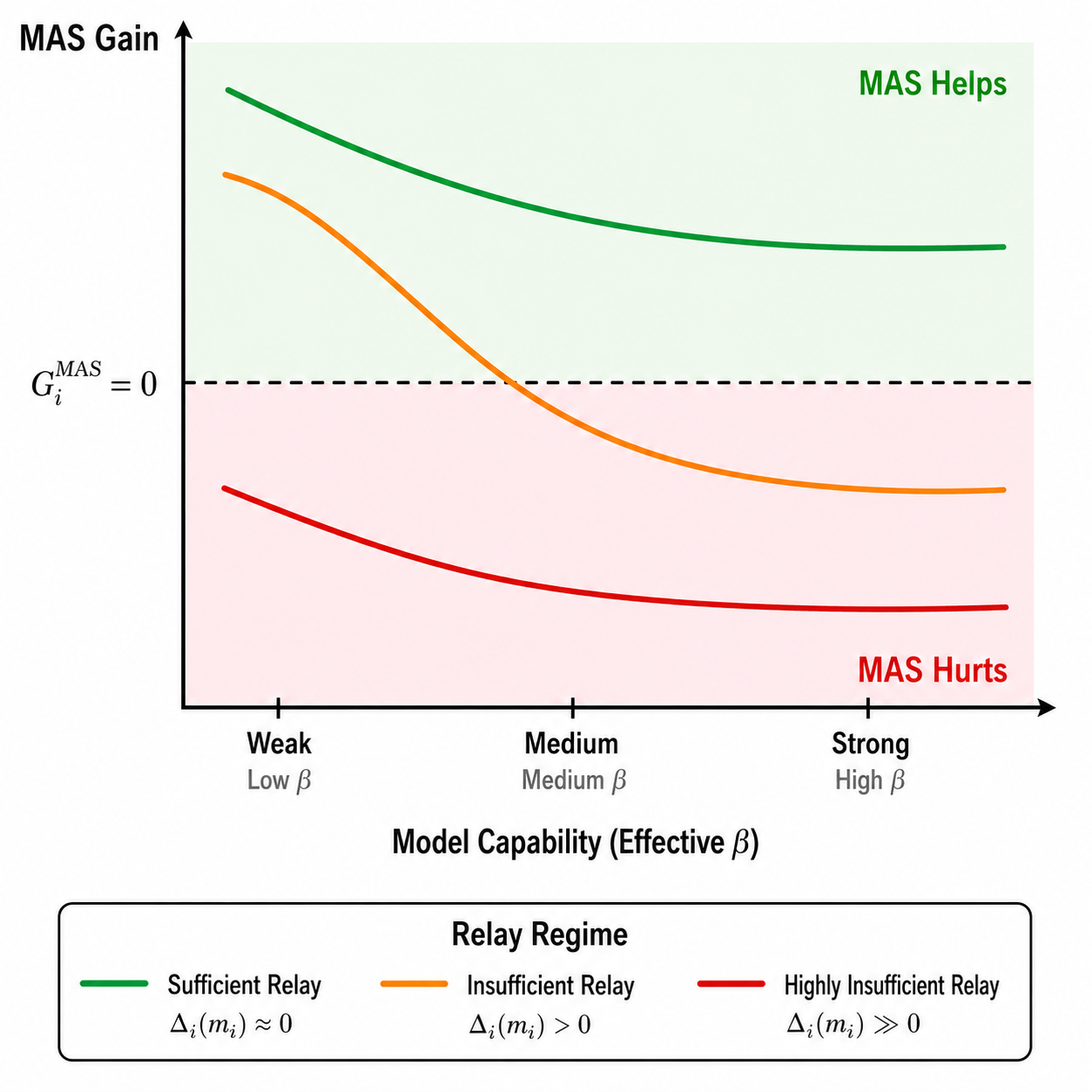
Figure 1 (paper Fig.1): MAS gain prediction by relay regime and capability.

Figure 2 (paper Fig.2): The three controlled prototypes side by side — SAS (single shared context), SAS-contextflow (same planner-induced decomposition, still one shared context), and MAS (same decomposition, but isolated worker contexts connected only by compressed relays $m_1, m_2$ ). This is the experimental design that isolates relay compression as the causal mechanism, described in the design-choice discussion above.

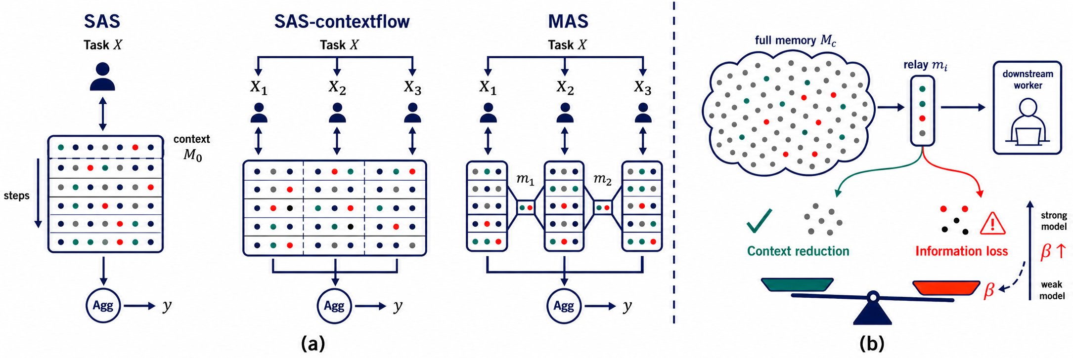
Figure 2 (paper Fig.2): Three controlled prototypes — SAS, SAS-contextflow, MAS.

Figure 3: A self-drawn diagram of the information flow inside a single MAS relay interface, matching Eqs. (1)-(7): worker $i$ ‘s full context $M_i$ is compressed by $\text{Agg}_i$ into relay $m_i$ , which alone (not $M_i$ ) is visible to worker $i+1$ , whose performance on target $Y_{i+1}$ depends on how much of $I(M_i;Y_{i+1}\mid X_{i+1})$ survived compression.

flowchart LR
    subgraph WorkerI["Worker i"]
        Mi["Full context M_i<br/>(all thoughts, actions, observations)"]
        Aggi["Aggregator Agg_i<br/>(compression / summarization)"]
        Mi --> Aggi
    end
    Aggi --> mi["Relay message m_i<br/>(bounded bandwidth B_sys)"]
    subgraph WorkerI1["Worker i+1"]
        Xi1["Sub-instruction X_(i+1)"]
        M0["Initial context M_0^(i+1) = (X_(i+1), o_0) ⊕ m_i"]
        Yi1["Downstream target Y_(i+1)"]
        Xi1 --> M0
        mi --> M0
        M0 -.affects.-> Yi1
    end
    Mi -. "cannot be seen by Worker i+1<br/>(only m_i is visible)" .-> WorkerI1

Figure 4 (paper Fig.3): Main empirical results across all five benchmarks and three model scales (Qwen2.5-7B, GPT-4o-mini, Qwen3.5-27B), with green/red shading showing where MAS outperforms or underperforms SAS-contextflow. This is the primary evidence for the paper’s central claim, discussed benchmark-by-benchmark in the Experiments section below.

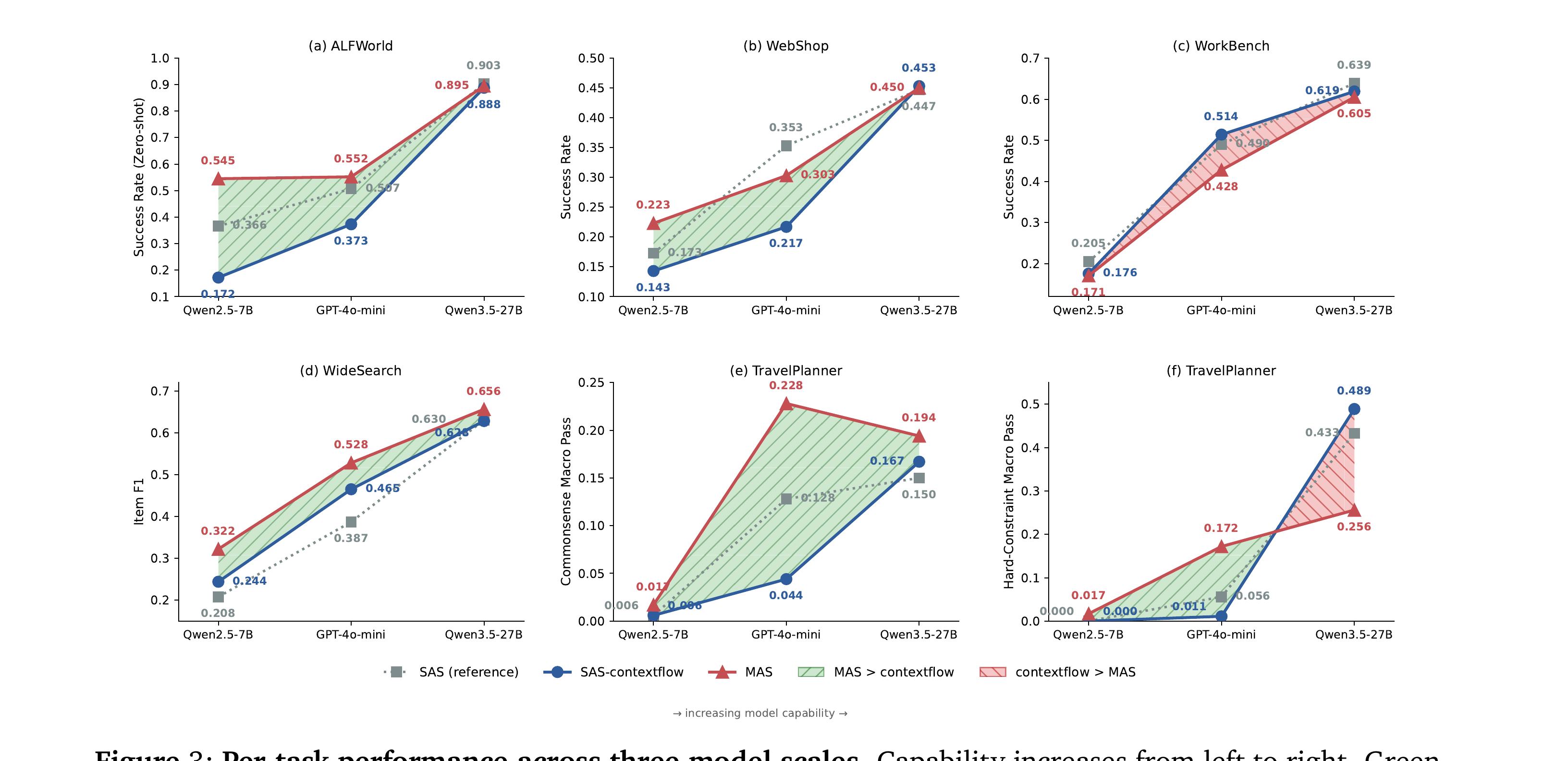
Figure 4 (paper Fig.3): Main results across benchmarks and model scales.

Figure 5 (paper Table 3, rendered as a figure): The SAS-Plan ablation, isolating whether planning structure alone (without context isolation) can explain MAS’s gains. SAS-Plan uses the same decomposed sub-instructions as MAS but keeps a single shared context, and it consistently underperforms plain SAS — direct evidence that decomposition alone is not the mechanism.

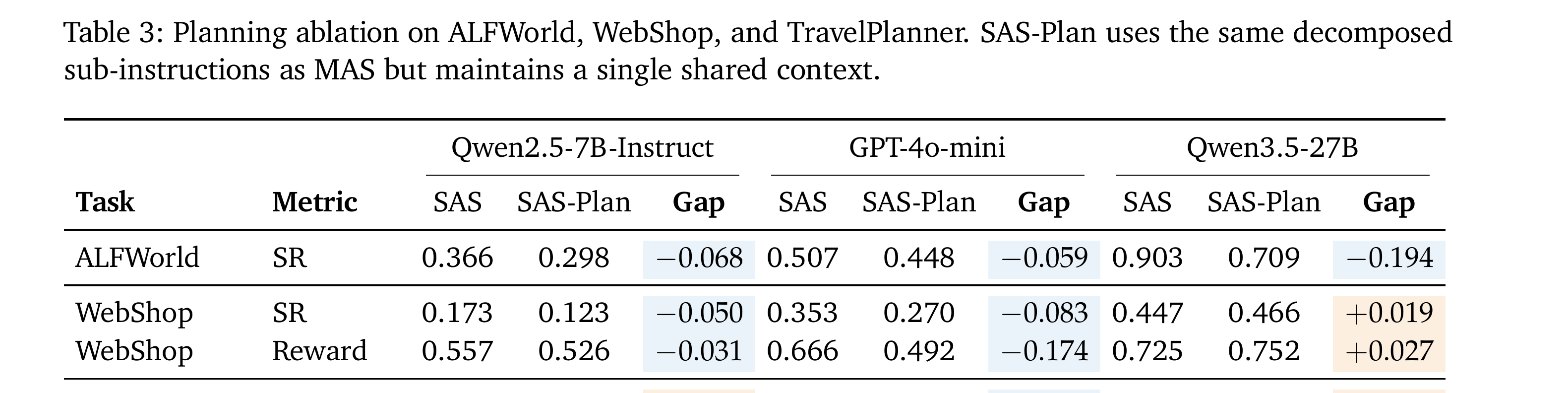
Figure 5 (paper Table 3): SAS-Plan ablation table.

Figure 6 (paper Table 4, rendered as a figure): The causal relay-sufficiency ablation on ALFWorld and WebShop, comparing a normal (“sufficient”) relay against a deliberately information-stripped (“insufficient”) relay at matched decomposition — the paper’s strongest causal evidence that $\Delta_i(m_i)$ operates as a genuine performance cost.

Figure 6 (paper Table 4): Relay sufficiency causal ablation table.

Experiments: Testing the Theory Against Five Benchmarks

Experimental Setup

The paper evaluates three controlled prototypes — SAS, SAS-contextflow, MAS — across three model scales spanning a real capability range: Qwen2.5-7B-Instruct (served locally via vLLM in bfloat16), GPT-4o-mini (via the OpenAI API), and Qwen3.5-27B using an AWQ 4-bit quantized checkpoint (also served locally via vLLM). All prototypes use greedy decoding (temperature 0.0) and are matched on total step budget per benchmark, so that MAS’s decomposition into multiple workers doesn’t get an unfair “more total compute” advantage over SAS.

Five benchmarks are chosen specifically to span a range of what the paper calls relay complexity, $\delta$ — informally, the minimum description length of a relay message that would be sufficient (i.e., $\Delta_i = 0$ ) for the downstream worker. ALFWorld (household navigation and manipulation tasks) and WideSearch (structured, mostly-independent information retrieval subqueries) are assigned $\delta \approx 0$ : their natural task structure means a short relay (e.g., “the object is on the shelf”) really can carry everything the next worker needs. WorkBench (multi-domain office-software tasks requiring exact prior read results like object IDs and timestamps before executing write actions) is assigned $\delta \gg 0$ : a bounded relay essentially cannot preserve everything a downstream write action needs. WebShop (search-then-purchase e-commerce) and TravelPlanner’s hard-constraint checks (global itinerary consistency, e.g., total budget across all days) sit in between, at $\delta > 0$ . TravelPlanner is treated specially as a mixed-regime benchmark: its commonsense checks (local feasibility of a single day’s plan) are $\delta \approx 0$ , while its hard constraints (global budget, cross-day consistency) are $\delta > 0$ — reported as separate CS-macro and HC-macro metrics.

Main Results: The Predicted Split Holds

Table 2 of the paper (not reproduced in full here, but summarized) groups all benchmarks by their assigned $\delta$ regime and reports MAS’s gain over SAS-contextflow at each of the three model scales. The pattern is remarkably clean:

For the low-complexity-relay benchmarks ( $\delta \approx 0$ ): ALFWorld shows MAS beating SAS-contextflow by +0.194, +0.157, and +0.023 (Qwen2.5-7B, GPT-4o-mini, Qwen3.5-27B respectively) — consistently positive, but shrinking as capability increases, exactly as Eq. (7) predicts (the same $H(M_i\mid m_i)$ benefit gets increasingly outweighed by a growing $\beta$ , even when $\Delta_i$ itself stays small). WideSearch shows the same qualitative pattern: +0.079, +0.063, +0.028 on Item F1. TravelPlanner-CS: +0.011, +0.183, +0.028.

For the high-complexity-relay benchmarks ( $\delta > 0$ or $\delta \gg 0$ ): WorkBench shows MAS losing to SAS-contextflow at every single model scale (-0.005, -0.086, -0.014) — the relay simply cannot preserve the exact object IDs, timestamps, and prior read results that downstream write actions require, so $\beta \Delta_i(m_i)$ dominates $H(M_i \mid m_i)$ regardless of model capability. WebShop and TravelPlanner-HC show the paper’s sharpest and most interesting pattern: a capability-dependent sign flip. WebShop goes from +0.080 and +0.086 (weak and medium models, where MAS still helps) to -0.003 on Qwen3.5-27B (where MAS starts to hurt). TravelPlanner-HC shows an even more dramatic flip: +0.017 and +0.161 for the two weaker models, collapsing to -0.233 for Qwen3.5-27B. This is precisely the qualitative signature Eq. (7) predicts: as $\beta$ grows with capability, the crossover point where $H(M_i\mid m_i) = \beta\Delta_i(m_i)$ can be crossed entirely, flipping the sign of the gain.

A Concrete Case Study: Watching the Sign Flip Happen

The paper includes a worked example (TravelPlanner task tp_1: a 3-day Oakland-to-Tucson itinerary under a hard $1,400 budget) that makes the abstract sign-flip tangible. The budget constraint is a *plan-level global* — it's never handed to any individual MAS sub-agent's sub-instruction, only tracked implicitly in the full context. On GPT-4o-mini (medium capability, smaller$ \beta $), SAS-contextflow's shared context gets cluttered enough that it leaves two of three days' accommodation slots empty (failing a validity gate before the budget check even runs), while MAS's isolated workers, each starting from a clean context, actually produce the only budget-valid itinerary — a case where context *reduction* clearly wins. On Qwen3.5-27B (high capability, larger$ \beta $), the pattern reverses: SAS-contextflow can hold onto and actively use the visible$ 1,400 cap throughout its long shared context and stays within budget, while MAS’s compressed relays lose the explicit budget figure by the final day and produce a $1,599 itinerary that fails the hard constraint. Same task, same budget number, same nominal "3-day itinerary" structure — opposite outcome, purely because the downstream model's capability moved the effective$ \beta$ across the crossover point in Eq. (7).

Ablation Studies: Isolating the Causal Mechanisms

Two further ablations sharpen the causal story. First, the planning-structure ablation (SAS-Plan, discussed above) shows decomposition alone, without context isolation, doesn’t explain MAS’s gains — SAS-Plan underperforms plain SAS on ALFWorld across all three models (-0.068, -0.059, -0.194), ruling out “breaking the problem into easier pieces” as the operative mechanism. Second, the relay-sufficiency ablation (Table 4) constructs “insufficient” relay variants by deliberately deleting downstream-required fields — object location and state for ALFWorld, price/attributes/navigation for WebShop — while holding the MAS decomposition otherwise fixed, and shows performance drops consistently across all model scales (e.g., ALFWorld SR drops by 0.015, 0.015, and 0.052 for the three models as relay sufficiency is degraded). This is the paper’s best direct evidence that $\Delta_i(m_i)$ isn’t just a mathematically convenient quantity that happens to correlate with performance — deliberately manipulating it causes the predicted performance change.

A Worked Numerical Sanity Check on the Gain Decomposition

It helps to plug in toy numbers to make Theorem 4.1 feel concrete rather than purely symbolic. Suppose, for a single relay interface, the full upstream context $M_i$ has entropy $H(M_i) = 10$ bits, and a candidate relay $m_i$ retains only $H(m_i) = 3$ bits of that (so $I(M_i; m_i) \le \min(H(M_i), H(m_i)) = 3$ bits in the best case, i.e., the relay is a deterministic function of $M_i$ , which is the typical case for a compressed summary). Then the upstream context reduction term is $H(M_i \mid m_i) = H(M_i) - I(M_i;m_i) = 10 - 3 = 7$ bits: seven bits’ worth of upstream clutter has been successfully stripped away. Now suppose the maximum possible downstream-relevant information available in $M_i$ is $I(M_i; Y_{i+1}\mid X_{i+1}) = 2$ bits, and the compressed relay manages to preserve $I(m_i; Y_{i+1}\mid X_{i+1}) = 1.5$ bits of that — so by Definition 4.1, $\Delta_i(m_i) = 2 - 1.5 = 0.5$ bits of downstream-relevant information were lost. Plugging into Eq. (7): MAS is beneficial at this interface exactly when $7 > \beta \times 0.5$ , i.e., when $\beta < 14$ . If the downstream model is weak enough that its effective $\beta$ sits well below 14 (it can’t exploit rich context anyway, so it doesn’t miss the lost 0.5 bits much), MAS wins comfortably. If the downstream model is capable enough that its effective $\beta$ climbs above 14 (it could have used that missing 0.5 bits productively), the same relay design flips to a net loss — this is the exact mechanism behind the WebShop and TravelPlanner-HC sign flips reported in the experiments, just with illustrative rather than measured numbers, since (as discussed in Limitations below) the paper does not actually estimate these bit quantities empirically.

Putting the Experimental Numbers in Perspective

It’s worth explicitly contrasting the magnitude of the gains and losses reported across regimes, since the raw numbers alone can undersell how sharp the qualitative pattern is. In the $\delta \approx 0$ regime, MAS’s advantage over SAS-contextflow is positive in all 9 reported cells (3 benchmarks × 3 models: ALFWorld, WideSearch, TravelPlanner-CS), with a mean gain across those cells of roughly +0.096 — a meaningful, double-digit-percentage-point improvement in several cases (e.g., +0.194 on ALFWorld with the weakest model). In the $\delta > 0$ / $\delta \gg 0$ regime, the picture inverts: WorkBench is negative in all 3 cells, and WebShop/TravelPlanner-HC together contribute 4 positive and 2 negative cells, with the 2 negative cells both occurring at the strongest model (Qwen3.5-27B) — exactly the models×benchmarks combination the theory says should be most exposed to relay information loss. This asymmetry (uniformly positive in the sufficient-relay regime, systematically flipping negative precisely at high capability in the insufficient-relay regime) is the paper’s strongest single piece of quantitative evidence, and it is considerably more convincing than looking at any individual benchmark’s numbers in isolation.

Reading the Case Study’s Table Carefully: What Actually Changed Between the Two Models

It is worth re-reading the TravelPlanner tp_1 case study (summarized above) once more, slowly, because it is easy to skim past exactly what changed between the GPT-4o-mini run and the Qwen3.5-27B run. The sub-task specifications handed to every worker (transport, accommodation, dining, attraction) are held fixed across both model runs — identical code-defined sub-specs, identical decomposition, identical relay boundaries. The only two things that differ are (a) which base model is doing the reasoning inside each worker, and (b) whether that specific model’s SAS-contextflow run happens to notice and retain the plan-level global budget figure of $1,400 in its accumulated context by the time it reaches the final consistency check. On GPT-4o-mini, this budget figure gets buried and functionally lost somewhere in the shared context (the paper attributes this to a validity-gate ordering issue: `is_not_absent` gates before `valid_cost` is even evaluated, so an incomplete plan never reaches the budget check at all), so MAS's clean, isolated per-day workers — which never had access to earlier days' accommodation decisions to get confused by — actually do better. On Qwen3.5-27B, the same$ 1,400 figure survives clearly in the long shared SAS-contextflow context (a stronger model is simply better at retaining and using a single salient number across a long context), while MAS’s relay-based workers lose track of the exact number by the final day and overshoot to $1,599. The lesson this drives home is that the paper's abstract$ \beta$ isn’t some mysterious latent trait — it cashes out concretely as “how good is this specific model at holding onto and using one important number across a long shared transcript,” a very down-to-earth capability that varies predictably with model scale and post-training quality.

Limitations

The authors are candid about several boundaries of their own framework, and it’s worth reading these carefully rather than skimming past them. First, $\beta$ is treated qualitatively, not quantitatively estimated — the paper never actually measures a numeric $\beta$ for any of the three models; it only asserts (and empirically confirms) that $\beta$ increases monotonically with capability. This means Theorem 4.1 gives you the direction of an effect but not a way to compute, in advance, exactly where the crossover point sits for a new task/model pair you haven’t yet tested. Second, relay complexity $\delta$ is assigned by qualitative task-structure analysis, not measured: the paper’s own five-benchmark taxonomy ( $\delta \approx 0$ , $\delta > 0$ , $\delta \gg 0$ ) is derived from the authors’ domain reasoning about what information each task’s downstream steps require, not from an automated or principled quantitative estimator. Third, the theory as stated is fundamentally a local, single-relay-interface result (Theorem 4.1 concerns one interface between worker $i$ and worker $i+1$ ); the paper’s own Section 4.2 “Local-to-Downstream Sufficiency” discussion shows that local sufficiency for the immediate next target does not automatically imply sufficiency for later downstream targets unless additional structural conditions (mediated dependence, non-interference) hold — meaning long chains of workers could have hidden long-range dependency failures the local theorem cannot catch by itself. Fourth, the model roster is limited to three specific checkpoints (Qwen2.5-7B, GPT-4o-mini, Qwen3.5-27B-AWQ-4bit) at a single point on each model’s release timeline — it’s an open question whether the capability- $\beta$ relationship generalizes smoothly across model families and post-training regimes, or whether some models could show non-monotonic behavior. Fifth, all relays and decompositions in the experiments are produced by fixed, hand-designed prompts (Appendix D), not learned or optimized relay encoders — the paper explicitly frames “jointly optimizing the relay with the downstream task” as future work rather than something it has already validated.

Critical Analysis

Weaknesses and flaws specific to this paper. The most significant technical gap is that the entire empirical validation rests on a qualitative proxy for the paper’s central quantitative claim. Theorem 4.1’s inequality, $H(M_i\mid m_i) > \beta \Delta_i(m_i)$ , is a precise, checkable statement about specific information-theoretic quantities — but the paper never actually estimates $H(M_i\mid m_i)$ , $\Delta_i(m_i)$ , or $\beta$ numerically for any real experiment. Instead, the empirical validation substitutes a rough five-level $\delta$ -regime taxonomy (assigned by the authors’ own judgment about task structure) and an implicit, unmeasured assumption that “capability” and " $\beta$ " move together. This is a real risk: the theory could be perfectly correct while the empirical support for it is closer to “a plausible qualitative story that fits the observed pattern” than to “a quantitatively validated causal model.” A more rigorous version of this paper would attempt to estimate mutual information terms directly — even crude estimators (e.g., using a smaller proxy model to compute conditional entropy over context/relay pairs, or using variational mutual information estimators like MINE or CLUB) would let the authors check whether the magnitudes of $H(M_i\mid m_i)$ and $\Delta_i(m_i)$ actually track the observed performance gaps quantitatively, not just directionally.

Limitations the authors understate or omit. The paper’s discussion of $\delta$ -regime assignment reads as more principled than it actually is upon close inspection — for instance, TravelPlanner is explicitly split into a “CS” ( $\delta \approx 0$ ) and “HC” ( $\delta > 0$ ) component, but this binary split is itself a judgment call about what counts as “local” versus “global” information, and a different, equally reasonable decomposition of the same task could plausibly be assigned differently. More importantly, the paper doesn’t seriously grapple with the possibility that its own controlled prototypes (SAS, SAS-contextflow, MAS) are not the only three interesting points in the design space — real production multi-agent systems often use hybrid designs (e.g., MAS workers that can request additional context on demand, or hierarchical designs where some workers share context and others don’t), and the paper’s clean three-way taxonomy doesn’t obviously extend to characterize these intermediate designs, even though they are arguably more representative of how MAS is actually deployed in practice. The paper’s Section 7 “Implications” gestures at “adaptive relays” as future work but doesn’t discuss what specific mechanism (learned compression? retrieval-augmented relays? on-demand context requests?) would actually move a design from one side of the crossover inequality to the other in a controllable way.

Concrete, specific improvement suggestions. (1) Add a direct, even approximate, estimation of the mutual-information quantities in Theorem 4.1 for at least one benchmark/model pair — for example, using a masked-language-model-based conditional entropy estimator over the actual context/relay text pairs collected during the WorkBench experiments, to check whether the sign and rough magnitude of $H(M_i\mid m_i) - \beta\Delta_i(m_i)$ actually track the observed MAS-vs-SAS-contextflow performance gap, rather than relying solely on the qualitative $\delta$ -regime taxonomy. (2) Extend the three-prototype comparison with at least one adaptive/hybrid relay design — e.g., a MAS variant where a worker can issue a follow-up query back to the previous worker if it detects that its relay was insufficient — to test whether the framework’s predictions extend cleanly to designs beyond the fixed, one-shot relay setting studied here. (3) Report an explicit estimate of relay message length (in tokens) alongside the $\delta$ -regime taxonomy for every benchmark, so readers can distinguish cases where MAS gains are being driven by genuine content-selection quality (the paper’s central claim) from cases where they might be confounded by simply “MAS relays happen to be shorter and thus less distracting,” which is a related but conceptually distinct effect the paper’s own Table 4 ablation gestures at but doesn’t fully disentangle from length effects. (4) Test at least one additional “in-between” capability point (e.g., a model between GPT-4o-mini and Qwen3.5-27B in raw capability) to check whether the crossover in WebShop and TravelPlanner-HC happens gradually (as Eq. 7’s smooth $\beta$ -dependence would predict) or more abruptly, which would materially affect how practitioners should reason about “is my model strong enough that MAS will start hurting me on this task.”

Connecting This to Prior MAS-vs-SAS Debates

The paper explicitly positions itself against a growing body of empirical work reporting that MAS gains “diminish as base model capability improves” (citing, among others, prior findings on multi-hop reasoning where a single strong agent matched or beat a multi-agent pipeline under equal thinking-token budgets). What this paper adds beyond that prior empirical literature is a mechanistic account of why that diminishing-returns pattern should occur, rather than just observing it. The key distinguishing move is decomposing the single empirical quantity “MAS gain” into two separately named, oppositely-signed components (upstream context reduction and capability-weighted relay loss), so that a diminishing MAS gain isn’t just an unexplained trend line but a predictable consequence of $\beta$ growing while $H(M_i\mid m_i)$ and $\Delta_i(m_i)$ stay comparatively fixed properties of the task’s relay design. This reframing also explains a detail prior empirical work left unresolved: why the diminishing-returns pattern isn’t universal — on the low-complexity-relay benchmarks (ALFWorld, WideSearch, TravelPlanner-CS) the paper’s own results show MAS gains shrinking with capability but never actually crossing zero within the tested range, while on the higher-complexity benchmarks the same shrinking trend does cross zero. Under the paper’s framework this is exactly what you’d expect: the crossover point in Eq. (7) depends on both $\beta$ and $\Delta_i(m_i)$ , and only when $\Delta_i(m_i)$ is large enough to begin with does a realistic amount of capability growth actually push $\beta \Delta_i(m_i)$ past $H(M_i\mid m_i)$ .

Conclusion

This paper answers a question that has been debated mostly with anecdote and vibes — “does splitting an LLM task across multiple agents actually help?” — with a genuinely mechanistic, checkable answer: it depends on whether your relay messages compress away noise faster than they discard signal, and that balance point shifts as your base model gets stronger. The theoretical core (Proposition 3.1’s equivalence result and Theorem 4.1’s gain decomposition) is elegant and, more importantly, directly falsifiable — the paper puts it through 18 controlled experiments and the predicted pattern holds up cleanly across benchmarks and model scales, including the striking capability-dependent sign flips on WebShop and TravelPlanner-HC. The most immediately useful practical upshot for anyone building agentic systems today: before reaching for a multi-agent architecture, ask whether the task’s natural decomposition would allow short, local, still-sufficient relay messages between workers — if downstream steps genuinely need detailed upstream evidence that’s expensive to summarize (like WorkBench’s exact object IDs and timestamps), a single agent with full shared context, especially if it’s already a strong model, may well outperform a fleet of specialized ones. The framework’s remaining gaps — no quantitative estimation of the theory’s own key terms, and no exploration of adaptive or hybrid relay designs — are exactly the directions that would turn this from a compelling explanatory lens into a practical, a-priori design tool.

A Note on Terminology: “Gain” vs. “Advantage” vs. “Improvement”

One small but genuinely useful clarification for readers coming from the broader multi-agent literature: the paper’s technical term “MAS gain” ( $G_i^{\text{MAS}}$ ) is a local, IB-objective-space quantity defined precisely by Eq. (6) — it is not the same thing as “the empirical performance improvement of MAS over SAS on benchmark X,” even though the two are closely related and the paper’s experiments treat the empirical success-rate delta as an observable proxy for the theoretical gain. This distinction matters because the theoretical $G_i^{\text{MAS}}$ is defined per-interface (i.e., local to one relay boundary between two specific consecutive workers), while the reported benchmark numbers (Table 2, Figure 3) are end-to-end task success rates that aggregate the effects of potentially several relay interfaces chained together (e.g., TravelPlanner’s five-phase decomposition in Table 5 has four relay interfaces in sequence). The paper’s Section 4.2 “Local-to-Downstream Sufficiency” discussion is precisely about this gap: a relay that is locally sufficient for the immediate next worker’s target is not automatically sufficient for a later worker’s target further down the chain, unless the specific mediated-dependence and non-interference conditions given in Appendix A.3 hold. Readers who want to map the paper’s clean theoretical story onto a real multi-hop MAS pipeline with more than two workers should keep this local-vs-global distinction in mind rather than assuming the single-interface theorem directly explains end-to-end multi-worker outcomes without further argument.

Reproducibility Notes

The paper reports a public GitHub repository (https://github.com/divelab/MAS-SAS) containing the experimental code. Model access requires either local vLLM deployment (for Qwen2.5-7B-Instruct and the Qwen3.5-27B-AWQ-4bit checkpoint, each runnable on a single NVIDIA RTX A6000 GPU per the paper’s Appendix B.2) or an OpenAI API key (for GPT-4o-mini). All five benchmarks used (ALFWorld, WebShop, WorkBench, WideSearch, TravelPlanner) are themselves public, previously released benchmarks with existing open-source harnesses, which should make re-running the core comparisons (with the paper’s own prompts, reproduced in Appendix D) feasible without needing to re-implement any bespoke evaluation infrastructure. One practical note for anyone attempting to reproduce results exactly: greedy decoding (temperature 0.0) is used throughout, which reduces run-to-run variance, but WideSearch specifically depends on a live DuckDuckGo web-search backend rather than an offline environment, meaning results on that specific benchmark may drift over time as underlying web content changes, unlike the other four benchmarks’ offline simulators/sandboxes.