Review date: 2026-07-24 Review author: Zhongzhu Zhou Paper reviewed: SVD-Surgeon: Optimal Singular-Value Surgery for Large Language Model Compression Paper authors: Mahmoud Safari, Frank Hutter arXiv: 2606.23568
Short Answer
Compressing a large language model with singular value decomposition (SVD) works by writing each weight matrix as and keeping only the top- singular values, throwing away the rest. Every existing SVD-based compression method — FWSVD, DRONE, ASVD, SVD-LLM, OBD-LLM — spends its cleverness on how to build that factorization (which basis to decompose in, how to weight it by activation statistics) and which singular values to discard. None of them ask a second, equally important question: once you’ve decided to throw some singular values away, should the ones you keep stay exactly as they were, or should they move to compensate for the ones you just deleted? SVD-Surgeon’s entire contribution is answering that second question with a closed-form, training-free formula. It imports the 1990s Optimal Brain Surgeon (OBS) idea — build a second-order (Hessian-based) model of how the loss changes when you perturb the model, and use it to compute the optimal compensating shift for the surviving parameters after pruning — but instead of applying OBS to individual weights (as GPTQ and SparseGPT do), it applies it to the singular values of a weight matrix, where is usually far smaller than the entries of the original matrix. This shrinks the relevant Hessian from an intractable object down to a manageable matrix that can be estimated from calibration gradients and inverted directly. The payoff, demonstrated by layering SVD-Surgeon on top of SVD-LLM (a strong existing SVD compressor) across the OPT family and LLaMA-2-7B: at aggressive 70% compression, WikiText-2 perplexity on OPT-6.7B drops from 944.57 (host method alone) to 46.36 — over 20× better — with no retraining, no gradient descent, and a single offline linear solve per layer.
Key Takeaways
- The core move is a change of basis, not a new compression algorithm. SVD-Surgeon does not compete with SVD-LLM, ASVD, or FWSVD on how to factorize weights — it sits on top of any of them, correcting the singular values they’ve already chosen to keep.
- The Hessian shrinks from to . By restricting the perturbation to changes in the singular values only (keeping the singular directions fixed), the fourth-order weight-space Hessian collapses to an ordinary matrix in singular-value coordinates — small enough to invert directly, unlike the weight-space Hessians that force GPTQ/SparseGPT-style methods into layer-wise diagonal or block approximations.
- The update is closed-form and training-free: , a single linear solve against a small, precomputed matrix — no iterative optimization, no backpropagation through the compressed model, no fine-tuning data beyond the calibration set already used to estimate the Hessian.
- The same math also yields a smarter pruning criterion. Instead of just ranking singular values by magnitude, the paper derives an OBS saliency that scores each value by the loss increase it would cause if removed and optimally compensated — a strictly more informative criterion when deviates from the identity.
- No orthonormality assumption is required. Because the derivation works for any factorization — not just the classical orthonormal SVD — SVD-Surgeon composes with SVD-LLM even though SVD-LLM’s whitening transform makes one of its two factors non-orthonormal. This generality is the mechanism that lets the method be a drop-in corrective layer rather than a from-scratch compressor.
- Gains are largest exactly where they matter most. Under mild compression (20–30%) there is little damage to compensate for, so the improvement is small. Under aggressive compression (60–80%), where naive truncation is catastrophic, SVD-Surgeon prevents the steep perplexity blow-up that the host method alone suffers.
- The method is honest about its own restriction. By design it updates only the singular values while freezing the singular directions — a deliberate simplification the authors flag explicitly as an open question (would jointly updating under the same second-order framework buy more?).
Cheat Sheet: The Method in One Paragraph
Before diving into the full prerequisites and derivation, here is the entire method compressed into a single paragraph you can return to as an anchor while reading the more detailed sections below. Given a weight matrix already decomposed as and already truncated to a retained set of singular values (discarding the complementary set ), SVD-Surgeon (1) collects per-sample calibration gradients via ordinary backward passes, (2) projects each into the singular-value basis via , (3) assembles a small empirical Fisher matrix , (4) partitions into retained/pruned blocks, and (5) solves the single linear system to get the optimal shift of the retained singular values. Optionally, the same also yields a saliency score that can replace the host method’s own pruning-set decision with one that accounts for post-compensation loss. Every subsequent section of this review is an expansion of one piece of this five-step recipe.
A Preview of the Argument’s Structure
This review is organized to mirror the paper’s own logical flow, but expands each stage considerably for a reader encountering these ideas for the first time. The Prerequisites section builds up, from first principles, everything needed to understand truncated SVD compression and classical Optimal Brain Surgeon independently, since the paper’s central contribution is precisely the fusion of these two previously separate ideas. The Architecture section gives a bird’s-eye view of the full pipeline before any equations appear, so that the subsequent three Method Parts (each corresponding to one major derivation in the paper’s Section 3) can be read with a clear sense of where each piece fits into the whole. The Experiments section then walks through every table and figure the paper reports, reproducing the exact numbers rather than paraphrasing them, so that a reader can independently verify the magnitude of the claimed improvements. Finally, the Critical Analysis section steps back from the paper’s own framing to ask what is missing, understated, or worth pressure-testing further — a perspective the paper itself, being a methods contribution rather than a critical survey, does not provide for itself.
Prerequisites: What You Need to Know First
Why Compress a Trained LLM at All
Large language models with tens or hundreds of billions of parameters are expensive to serve: every forward pass streams the full weight matrices from GPU memory, and inference on commodity or edge hardware is often bottlenecked by how much memory those weights occupy, not by raw compute. Post-training compression tries to shrink a pretrained model — no retraining from scratch — so it fits in less memory and runs faster, while degrading task performance (usually measured by perplexity on a held-out text corpus) as little as possible. There are three broad families:
- Structured pruning — remove entire neurons, attention heads, or layers. Hardware-friendly (no special kernels needed) but coarse-grained: removing a whole head or layer is a big, blunt cut that often hurts quality noticeably.
- Unstructured pruning — zero out individual weight entries based on some importance score. Fine-grained and can preserve quality well, but produces an irregular sparsity pattern that ordinary dense-matrix hardware cannot exploit for a real speedup without specialized sparse kernels.
- Low-rank (SVD) compression — approximate each weight matrix by a low-rank factorization with rank . This is attractive because it is naturally hardware-friendly: a rank- factorization is just two ordinary dense matrix multiplications ( then ), no custom kernel required, and the parameter count drops from to .
SVD-Surgeon lives in the third family. It is worth being precise about what “SVD compression” means here: for any matrix , the singular value decomposition writes where , have orthonormal columns, , and with . Truncating to rank means keeping only the top- singular values/vectors and zeroing the rest; by the Eckart–Young theorem this is the provably optimal rank- approximation of in Frobenius norm (i.e., treating every weight coordinate as equally important). The trouble is that “equally important in Frobenius norm” is not the same as “equally important to the model’s actual task loss” — a singular value can be numerically small yet correspond to a direction the network relies on heavily, or numerically large yet nearly irrelevant to the final loss. This mismatch is exactly what an entire sub-field (which this paper’s Related Work section surveys) has been trying to fix.
The Compression Ratio and How Rank Maps to It
For a weight matrix of shape , a rank- factorization stores numbers instead of . The paper defines the compression ratio as the fraction of parameters removed:
Solving for given a target :
rounded to the nearest integer, computed per layer (since differ across layers). The experiments in this paper sweep from 0.2 (mild — remove 20% of parameters) to 0.8 (very aggressive — remove 80%), with the interesting behavior concentrated in the 0.5–0.8 range where naive truncation starts to hurt badly.
Prior Art: Making Truncation “Aware” of Something
Naively truncating to the smallest singular values, as vanilla truncated SVD does, ignores everything about how the weight matrix is actually used downstream — it is purely a property of the matrix in isolation. A line of prior work tries to make the truncation aware of the model’s actual behavior:
- FWSVD reweights the weight matrix by an estimate of Fisher importance before decomposing, so that entries the model is more sensitive to get preserved more faithfully.
- DRONE minimizes the output approximation error (how different the layer’s output activations are, not just the weights themselves) using the empirical input activation distribution.
- ASVD scales the weight matrix by activation statistics before decomposing, effectively re-weighting each column by how large the typical activation passing through it tends to be.
- SVD-LLM, the “host” method this paper builds on, introduces a truncation-aware data whitening transform: it factors the input activation Gram matrix via a Cholesky decomposition, and shows that decomposing the whitened weight rather than itself yields the factorization that is optimal for the actual layer reconstruction loss (not just the raw weight-matrix Frobenius norm). It additionally recovers some of the lost accuracy with LoRA-style fine-tuning of the truncated factors.
- OBD-LLM goes further and uses a Kronecker-factored (K-FAC) approximation of the task-loss Hessian to build a bidirectional (both input- and output-aware) whitening transform.
All five of these methods share a common shape: they change how the factorization is constructed — which basis, which weighting — so that the singular values that end up small really are small in terms of task loss, not just Frobenius norm. But once that factorization is fixed and a rank cutoff is chosen, all of them simply discard the pruned singular values and leave the retained ones untouched. This is exactly the gap SVD-Surgeon fills: given any such factorization and truncation, can the retained singular values be nudged to actively compensate for what was just thrown away?
Optimal Brain Surgeon (OBS): The Idea SVD-Surgeon Imports
Optimal Brain Surgeon dates back to 1992 (Hassibi & Stork) and has recently been revived at LLM scale by methods like GPTQ, SparseGPT, Optimal Brain Compression, and the Optimal BERT Surgeon. The core idea: near a trained (locally optimal) point, the gradient of the loss is approximately zero, so a second-order Taylor expansion of the loss around a small perturbation is dominated by the quadratic (Hessian) term:
where is the Hessian of the loss with respect to the parameters. If you partition the parameters into a set you plan to keep and a set you plan to prune (set to zero), OBS asks: given that is being zeroed, what is the loss-minimizing adjustment of the surviving parameters? This has a clean closed-form answer (derived via Lagrange multipliers in the classical treatment, and via direct substitution in this paper — see Method Part 2 below), and it also yields a saliency score — the loss increase incurred by removing any one parameter, after applying the optimal compensation to the rest — that is a strictly better pruning criterion than raw magnitude whenever the Hessian is not close to a scaled identity matrix.
The catch, historically: for a weight matrix with entries, the naive Hessian has entries — utterly intractable to store or invert for realistic LLM layer sizes. Every prior OBS-style method (GPTQ, SparseGPT, LLM Surgeon) has had to introduce some structural approximation — a diagonal Hessian, a layer-wise input Gram matrix as a proxy Hessian, a Kronecker-factored curvature — to make the linear algebra tractable at all. SVD-Surgeon’s key insight is that if you change coordinates first — from individual weight entries to singular values — the effective Hessian shrinks dramatically, because there are only singular values instead of individual weight entries. This is the central trick the rest of the method builds on.
The Eckart-Young Theorem and Why It Matters Here
One classical result underlies the entire discussion of truncated SVD’s optimality (and sub-optimality) in this review: the Eckart-Young-Mirsky theorem. It states that among all rank- matrices , the truncated SVD (keeping the top- singular values and setting the rest to zero) minimizes the Frobenius-norm reconstruction error , and this minimum is achieved by no other rank- matrix. This is a genuinely strong, provably optimal guarantee — but its optimality is scoped narrowly to the Frobenius norm of the raw weight matrix, treating every entry as equally important. Every method surveyed in Prerequisites (FWSVD, DRONE, ASVD, SVD-LLM, OBD-LLM) is, in one way or another, working around this narrow scope: each one either reweights the matrix before applying Eckart-Young (so the theorem’s optimality guarantee now applies to a different, more task-relevant matrix), or works with a different loss altogether. SVD-Surgeon does something different again: it accepts whatever truncation the host method already computed (which may or may not have already applied Eckart-Young to a reweighted matrix), and instead of trying to get the truncation itself “more optimal,” it asks whether the survivors of a fixed truncation can be adjusted to reduce the loss further. This framing helps explain why SVD-Surgeon composes so cleanly with the entire prior-art family: it doesn’t compete with Eckart-Young-style optimality claims at all, it operates one step downstream of them.
Deeper Dive into Each Prior-Art Method
The Prerequisites section above summarized each prior method in a sentence; it is worth unpacking a few of them slightly further, since understanding why each one improves on naive truncation clarifies exactly what gap SVD-Surgeon fills.
FWSVD’s Fisher reweighting in more detail. Naive SVD minimizes , treating every entry of as equally important. FWSVD instead minimizes a weighted Frobenius norm , where is built from an estimate of each weight’s Fisher importance (how much perturbing that weight would change the loss, to first order). This changes the effective SVD problem being solved without changing the shape of the solution — it’s still a truncated SVD, just of a reweighted matrix. Note the family resemblance to SVD-Surgeon: both use Fisher-style importance information, but FWSVD folds it into the initial decomposition (changing what counts as “small” before any truncation happens), while SVD-Surgeon acts entirely after a decomposition and truncation have already been fixed, repairing the survivors rather than reshaping the whole problem upfront.
SVD-LLM’s whitening in more detail. The key move is recognizing that the weight-space Frobenius error is the wrong thing to minimize if what you actually care about is the layer’s output on real data, . SVD-LLM’s insight is that this output-error objective can be converted back into an ordinary (unweighted) Frobenius-norm SVD problem, just on a transformed matrix: whitening by the Cholesky factor of makes the natural object to decompose, because exactly (a consequence of having identity covariance). This is an elegant reduction — it means SVD-LLM doesn’t need any new algorithm, just a change of variables before calling ordinary truncated SVD, then a change back afterward. This is also exactly why SVD-LLM’s right factor ends up non-orthonormal (Application to SVD-LLM section above), and why testing SVD-Surgeon on it is a meaningful stress test of the “no orthonormality required” claim rather than a convenient toy case.
Architecture and Data-Flow Overview
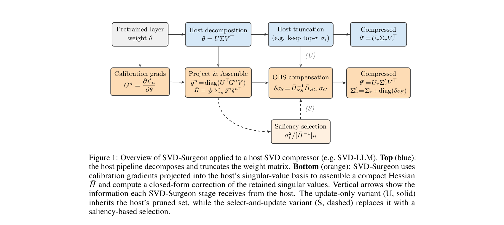
Figure 1 below (reproduced from the paper) shows the whole pipeline end to end. The top row (blue) is the “host” SVD compressor’s existing pipeline — decompose, then truncate. The bottom row (orange) is what SVD-Surgeon adds: it reads calibration gradients, projects them into the host’s own singular-value basis, assembles a compact Hessian , and computes a closed-form correction of the retained singular values. Two variants are shown: the solid arrow path (U, update-only) inherits whatever pruned set the host method already chose and only adds the compensation; the dashed arrow path (S, select-and-update) additionally re-derives which singular values to prune using the OBS saliency, before applying the same compensation formula.
Figure 1 (paper Fig.1): SVD-Surgeon applied to a host SVD compressor.
flowchart LR
    A["Pretrained weight θ (m×n)"] --> B["Host decomposition θ = UΣVᵀ"]
    B --> C["Host truncation: keep top-r σᵢ"]
    C --> D["Naive compressed θ' = Uᵣ Σᵣ Vᵣᵀ"]

    A --> E["Calibration gradients Gⁿ = ∂Lₙ/∂θ"]
    E --> F["Project into singular-value basis: ḡⁿ = diag(UᵀGⁿV)"]
    F --> G["Assemble compact Hessian H̄ = (1/N) Σₙ ḡⁿ ḡⁿᵀ"]
    G --> H["OBS compensation δσ_S = H̄_SS⁻¹ H̄_SC σ_C"]
    C -.-> H
    H --> I["Repaired compressed θ' = Uᵣ Σᵣ' Vᵣᵀ, Σᵣ' = Σᵣ + diag(δσ_S)"]

    G --> J["Saliency selection: σᵢ² / [H̄⁻¹]ᵢᵢ"]
    J -.->|"replaces host's pruned set (variant S)"| H
Note the two vertical dashed/solid arrows in the paper’s figure: this is precisely the fork between the update-only (U) and select-and-update (S) variants described in the Key Takeaways. Both share the exact same compensation math; they differ only in whether the “which singular values to prune” decision comes from the host method (U) or from SVD-Surgeon’s own saliency (S).
Why This Matters for the Broader Field of Efficient Deep Learning
Before diving into the mathematical core of the method, it’s worth situating why a paper about a fairly narrow technical correction to SVD compression matters beyond its immediate numbers. The broader context is that LLM compression research has, for several years, largely treated “how to factorize” and “what to discard” as the only two levers worth pulling — an entire generation of methods (surveyed in Prerequisites above) competes purely on refining these two choices. SVD-Surgeon’s contribution is conceptually orthogonal: it identifies and formalizes a third lever — “how to repair what’s left” — that the field had largely left unaddressed, not because it’s hard to imagine, but because doing it exactly (rather than heuristically) requires the specific dimensional-reduction insight (projecting into the singular-value basis before attempting Hessian-based reasoning) that this paper introduces. This is a useful reminder that even in a well-studied area, restructuring the coordinate system in which a classical technique (OBS) is applied can unlock capabilities that were computationally out of reach in the original coordinate system.
Method Part 1: Reducing the Hessian to the Singular-Value Basis
Step-by-Step Derivation
This is the mathematical heart of the paper, so it is worth walking through carefully, matching the paper’s own notation.
Step 1 — restrict the perturbation to singular-value changes only. SVD-Surgeon does not touch the singular directions — those stay exactly as the host method produced them. The only degrees of freedom being perturbed are the diagonal entries of . Writing , the induced weight perturbation is
Step 2 — substitute into the generic quadratic loss model. Recall from Prerequisites that is kept in native matrix form (not vectorized), so the weight-space Hessian is a fourth-order tensor , and the quadratic loss model reads
Substituting (and similarly for with a dummy index ):
Step 3 — pull the scalars outside the sum over matrix indices. Since don’t depend on , they factor out, leaving:
where the paper defines the projected Hessian entry
Step 4 — recognize the collapsed quadratic form. The whole fourth-order sum has collapsed into an ordinary quadratic form in the -dimensional vector :
Why this matters practically: is only , where — typically in the thousands for a transformer weight matrix — instead of , which for a matrix would be a object. This dimensional collapse is the mechanism that makes an exact (not diagonal-approximated, not Kronecker-approximated) Hessian inversion computationally feasible.
Design Choice: Why Freeze and Only Update ?
Why it works: Restricting the perturbation to alone is precisely what collapses the fourth-order tensor into the small matrix in Step 3–4 above. If and were also allowed to vary, the perturbation would live in an -dimensional space (or more, if the SVD’s orthonormality constraints are also relaxed), and the corresponding Hessian block would again be far too large to invert directly, undoing the whole point of the reduction.
The obvious alternative: allow the singular directions to shift too, and solve a larger joint OBS problem over . The paper explicitly flags this as future work — “relaxing the fixed-direction assumption to allow joint updates of within the same second-order framework could close the gap left by freezing the singular directions” — but notes it is an open question whether the (much higher) computational cost is justified by the gain.
Where it fails / boundary condition: freezing means SVD-Surgeon can only correct for damage that is expressible as a rescaling of the existing singular directions. If the ideal post-truncation correction actually requires rotating the singular subspace (e.g., redistributing information into a slightly different set of directions than the ones the host method happened to keep), no amount of rescaling the retained can reach that solution. The experiments (Section 4) show this restriction is not fatal in practice — the gains are still large — but it does bound how much further improvement any -only method (SVD-Surgeon included) can achieve on a given host factorization.
An Aside: What Does It Mean for to Equal the Exact Hessian?
One subtle but important claim buried in Method Part 1’s Step 4 deserves its own spotlight: the paper states that , despite being derived via a Fisher (first-order, outer-product) approximation, actually coincides with the exact loss Hessian in singular-value coordinates, . This is worth unpacking, because at first glance it seems to conflict with the Fisher approximation being, in general, only an approximation to the true Hessian in weight space.
The resolution is that the weight-space Fisher approximation (Equation 10, ) is indeed only an approximation — it assumes the model is near a local optimum so the true gradient is negligible, which lets the empirical covariance of gradients stand in for the true curvature. This approximation error does not vanish when projected into singular-value coordinates; what the paper is claiming is narrower and more precise: given that this Fisher approximation to has already been accepted as the working model of curvature, the corresponding projection (via the chain-rule identity ) computes exactly the same object you would get by directly differentiating twice with respect to under that same Fisher model — there is no additional approximation error introduced by the projection step itself. In other words: the Fisher approximation to the true Hessian is inherited, unchanged, from the weight-space assumption; the singular-value-space reduction adds no further error on top of it. This is a reassuring but modest claim — it says the coordinate change is lossless given the Fisher assumption, not that the Fisher assumption itself is accurate.
Method Part 2: Fisher Approximation of the Hessian
Why an Approximation Is Needed at All
Equation (9) requires the true Hessian . Computing exact second derivatives is expensive and awkward — most autodiff frameworks don’t expose directly, since isn’t a native parameter of the underlying network (the network’s actual parameters are the raw weight matrix entries ). So the paper reaches for the standard near-convergence approximation: the empirical Fisher information, a sum of outer products of per-sample gradients.
Step-by-Step Derivation
Step 1 — approximate the weight-space Hessian by the empirical Fisher. Near a converged (or well-trained) point, the per-layer Hessian is approximated as
where is the loss on calibration sample and is the number of calibration samples.
Step 2 — substitute into the definition of and simplify. Plugging the Fisher approximation into :
Step 3 — factor the sum, since and each appear only in one gradient factor. The double sum over (attached to ) and (attached to ) separates cleanly:
Step 4 — define the projected gradient and write in matrix form. Setting (i.e., the -th diagonal entry of the gradient projected into the basis):
Intuition, and why this is computationally cheap: by the chain rule and , the quantity is exactly — the singular-value gradient — even though it was never computed via any second-derivative machinery. Autodiff frameworks readily hand you the full weight-space gradient (a standard first-order operation); getting from it is then a single matrix product followed by extracting the diagonal — no second derivatives are computed anywhere in the pipeline, even though turns out to equal the exact loss Hessian in singular-value coordinates.
Design Choice: Why Fisher, and What’s the Alternative?
Why it works: the empirical Fisher information is a standard, well-understood surrogate for the true Hessian near a local optimum, used throughout the OBS literature (Optimal BERT Surgeon, Optimal Brain Compression, GPTQ, SparseGPT all use variants of this idea). It only requires first-order gradients, which every training/inference framework computes cheaply and natively.
The obvious alternative: compute the exact second derivatives directly (e.g., via Hessian-vector products or finite differences). The paper notes coincides with this exact Hessian under the Fisher approximation’s assumptions, so there is little to gain from paying the extra cost of true second-order autodiff, and considerable cost to avoid — Hessian-vector products for each of the basis directions would multiply the compute cost significantly.
Where it fails / boundary condition: the Fisher approximation assumes the model is near a local loss minimum (so the true gradient is negligible and the loss landscape is locally well-described by its Hessian). It also assumes block-diagonality of the Hessian across layers — i.e., that cross-layer curvature terms can be ignored and each layer’s can be estimated independently. Both are standard simplifying assumptions in this literature, but they are assumptions, not guarantees; if calibration data is not representative of deployment data, the estimated will not reflect the true deployment-time loss landscape, and the “optimal” compensation will be optimal with respect to the wrong objective.
Math-Visualizing Figure: The Block Partition of the Hessian
The entire compensation-and-saliency derivation in Method Part 3 hinges on partitioning the small Hessian into four blocks according to which singular values are retained () versus pruned (). The diagram below visualizes this partition and which block feeds into which formula — it is the structure underlying both Equation (15) (the compensation) and Equation (20) (the saliency).
flowchart TB
    subgraph HBlocks["ℓ×ℓ empirical Fisher H̄, partitioned by retained set S (size r) and pruned set C (size ℓ-r)"]
        direction LR
        HSS["H̄_SS  (r × r)\nretained-retained block\nneeds only ONE inverse for compensation (Eq. 15)"]
        HSC["H̄_SC  (r × (ℓ-r))\ncross block\nmultiplies σ_C in Eq. 15"]
        HCS["H̄_CS = H̄_SC^T"]
        HCC["H̄_CC  ((ℓ-r) × (ℓ-r))\npruned-pruned block\nnaive cost of removing σ_C alone"]
    end
    HSS --> Comp["δσ_S* = H̄_SS⁻¹ H̄_SC σ_C   (Eq. 15, update-only path)"]
    HSC --> Comp
    HCC --> Schur["Schur complement: H̄_CC − H̄_CS H̄_SS⁻¹ H̄_SC"]
    HCS --> Schur
    HSS --> Schur
    HSC --> Schur
    Schur -->|"block-inversion identity"| Saliency["[H̄⁻¹]_CC⁻¹  →  per-value saliency σ_i² / [H̄⁻¹]_ii   (Eq. 20, select-and-update path)"]
Reading this diagram alongside the derivation: the update-only variant (U) only ever needs and — the two blocks touching the retained set — which is why it is the cheaper of the two variants (Figure 3 below quantifies this cost gap directly). The select-and-update variant (S) additionally needs the full Schur complement (touching all four blocks) to compute a saliency for every singular value, retained or not, which is why it requires inverting the full rather than just the sub-block.
Connecting the Dots: How the Saliency Generalizes Magnitude Pruning
Before diving into the full derivation, it is worth sitting with the special-case result mentioned in Key Takeaways — that the OBS saliency reduces to plain magnitude-squared, , when — a bit longer, because it is the cleanest way to build intuition for what the saliency formula is really doing before working through the full block-matrix algebra.
Imagine the Hessian were exactly the identity matrix. This would correspond to a hypothetical world where perturbing any one singular value has a loss impact completely independent of, and identical in scale to, perturbing any other singular value — no cross-coupling, no varying sensitivity. In that world, there would be no reason to prefer a loss-aware criterion over raw magnitude: every singular value contributes the same per-unit-magnitude loss impact, so ranking by directly ranks by loss impact, and there is nothing for a smarter criterion to correct for. The real value of the saliency formula only appears once deviates from this idealized case — once some singular-value directions are more “loss-sensitive” than others (large diagonal entries, small ) or are strongly coupled to their neighbors (large off-diagonal entries), at which point a numerically small can still carry a large loss cost, or a numerically large can be safely removed because its role is easily absorbed by a correlated neighbor. This is the same intuition that motivates every OBS-family method over naive magnitude pruning, just instantiated here in the much smaller singular-value coordinate system rather than the original weight-entry coordinate system.
Method Part 3: The Closed-Form Update and the Saliency Score
Algorithm 1 — Optimal Compensation (Update-Only Variant)
Algorithm 1: SVD-Surgeon compensation (update-only, U)
Input:  weight θ ∈ R^{m×n}; host decomposition θ = U Σ V^T;
        host-chosen retained set S, pruned set C (|S| = r);
        calibration gradients {G^n}_{n=1..N}
Output: repaired compressed weight θ' = U_r Σ_r' V_r^T

1:  for n = 1 to N:
2:      compute G^n = ∂L_n/∂θ                      # standard backward pass
3:      ḡ^n ← diag(U^T G^n V)                        # project into singular-value basis
4:  H̄ ← (1/N) Σ_n ḡ^n ḡ^{nT}                          # assemble ℓ×ℓ empirical Fisher
5:  partition H̄ into blocks H̄_SS, H̄_SC, H̄_CS, H̄_CC   # conformal to (σ_S, σ_C)
6:  add diagonal damping d_S to H̄_SS                 # numerical stability (Section 4.1)
7:  δσ_S ← λ · H̄_SS^{-1} H̄_SC σ_C                    # closed-form compensation, scaled by λ
8:  Σ_r' ← Σ_r + diag(δσ_S)                          # repaired retained singular values
9:  θ' ← U_r Σ_r' V_r^T                              # assemble repaired compressed weight
10: return θ'
Derivation of the Closed-Form Update
Step 1 — expand the quadratic loss model over the partition . Substituting the block partition into Equation (9):
Step 2 — impose the pruning constraint. Pruning to zero means (the change needed to bring from its current value down to zero). Rather than handling this constraint via a Lagrange multiplier (the classical OBS derivation), the paper substitutes it directly, turning the problem into an unconstrained minimization over alone:
(The term from Equation 13 is dropped because it does not depend on and is therefore irrelevant to the minimization.)
Step 3 — set the gradient to zero. Differentiating the bracketed expression in (14) with respect to and setting it to zero:
This is the entire compensation formula: a single linear solve against the block (where is the number of retained singular values), multiplied by the cross-block applied to the values being removed, .
Derivation of the Saliency Score
Step 1 — substitute the optimal compensation back into the loss expansion. Plugging (15) back into (13) and simplifying (the algebra collects terms and uses ):
Step 2 — recognize the Schur complement. The matrix in parentheses, , is exactly the Schur complement of inside . Intuitively: alone would be the naive cost of removing with no compensation at all, and the subtracted term is the reduction in that cost afforded by optimally shifting the survivors.
Step 3 — rewrite using block-matrix inversion. By the standard block-inversion identity, , so the loss increase can be rewritten as
This is exactly the classical OBS saliency result, re-derived here in the singular-value basis rather than via the original Lagrange-multiplier route.
Step 4 — specialize to removing a single singular value. If is a single index, Equation (19) collapses to the simple, per-value score:
Intuition: this scores each singular value by the loss it would cause if pruned and optimally compensated for — not just by its raw magnitude. Note the special case: if (the identity), then and the saliency reduces to , i.e., ordinary magnitude-based selection. This shows explicitly that magnitude-based pruning is a special case of the OBS saliency — it is only optimal when the loss landscape happens to be locally isotropic in singular-value coordinates, which is generally not true.
Algorithm 2 — Select-and-Update Variant
Algorithm 2: SVD-Surgeon select-and-update (S)
Input:  weight θ ∈ R^{m×n}; host decomposition θ = U Σ V^T;
        target rank r; calibration gradients {G^n}_{n=1..N}
Output: repaired compressed weight θ' = U_r Σ_r' V_r^T

1:  compute H̄ as in Algorithm 1, lines 1-4
2:  add diagonal damping d to H̄ (full ℓ×ℓ matrix)
3:  for i = 1 to ℓ:
4:      saliency_i ← σ_i^2 / [H̄^{-1}]_ii             # Equation (20), requires H̄^{-1}
5:  C ← indices of the (ℓ-r) lowest-saliency values  # replaces the host's pruned set
6:  S ← remaining r indices
7:  apply Algorithm 1, lines 5-10, with this new (S, C) partition
8:  return θ'
Design Choice: Update-Only vs. Select-and-Update — Why Two Variants?
Why update-only (U) works and is cheap: it inherits whatever pruned set the host method already committed to (e.g., SVD-LLM’s own truncation-aware criterion), and only solves the single linear system in line 7 of Algorithm 1 against the block . This is the cheaper of the two variants and, per the paper’s own ablation (Section 4.2), captures “most of the improvement.”
The obvious alternative — select-and-update (S): don’t trust the host’s pruning criterion at all; re-derive it from the OBS saliency, which is provably the loss-optimal criterion under the second-order model. This requires inverting the full (block-truncated) to compute the per-value saliency scores in Equation (20) for every candidate, which is more expensive (Figure 2, discussed below, shows this cost difference directly).
Where each fails / boundary condition: the paper’s own results (Table 1) show that (S) adds only “a smaller, further gain in most settings” over (U) — the two variants track each other closely (Figure 3 only plots U, noting S is visually indistinguishable at that scale). This suggests that, at least for SVD-LLM as the host, the pruning-set decision was already reasonably close to loss-optimal, and most of the available improvement comes from repairing the survivors rather than choosing a different survivor set. This is a useful negative result: it means practitioners who want the bulk of the benefit at the lowest engineering cost can adopt update-only (U) and skip the more expensive saliency computation.
Recapping the Full Derivation Chain in One Table
Given the density of the preceding three Method sections, it may help to see the entire derivation chain summarized as a single sequence of steps, from the generic quadratic loss model down to the final closed-form update and saliency score:
| Step | What happens | Equation |
|---|---|---|
| 1 | Generic second-order loss model for any parameter perturbation | (1) |
| 2 | Restrict to weight matrices in native (non-vectorized) form | (2) |
| 3 | Restrict the perturbation to singular-value changes only, | (3)-(8) |
| 4 | Collapse the fourth-order weight-space Hessian into an matrix | (9) |
| 5 | Approximate the true Hessian via empirical Fisher information from calibration gradients | (10)-(12) |
| 6 | Partition into retained/pruned blocks and expand the loss model | (13) |
| 7 | Substitute the pruning constraint , minimize over | (14) |
| 8 | Solve for the closed-form optimal compensation | (15) |
| 9 | Substitute back to get the residual loss (Schur-complement form) | (16)-(19) |
| 10 | Specialize to single-index saliency for pruning-set selection | (20) |
Every one of these ten steps was walked through individually in Method Parts 1 through 3 above; this table exists purely as a navigational aid for readers who want to trace a specific number in the Experiments section back to the exact point in the derivation where it originates.
Application to SVD-LLM: A Non-Trivial Compatibility Test
The paper chooses SVD-LLM as its host not just because it is a strong baseline, but because SVD-LLM’s decomposition is a genuinely useful stress test of the “no orthonormality required” claim. Recall SVD-LLM’s construction: it whitens the input activations via a Cholesky factor of the Gram matrix (), decomposes the whitened weight , truncates , and maps back through the inverse whitening transform:
Cast in the general form , the left factor remains orthonormal (it comes from a standard SVD of the whitened matrix), but the right factor absorbs the inverse whitening transform and is no longer orthonormal — in general. Because the entire SVD-Surgeon derivation (Steps 1–4 of Method Part 1) never invoked or anywhere, the compensation formula (15) applies unchanged to this non-orthonormal . This is precisely the generality the paper’s Contributions section advertises, demonstrated on a real, widely-used method rather than a toy example.
Before vs. After: A Concrete Illustration Using the Toy Example
It helps to see the “before” and “after” states side by side using the numbers from the worked example in Method Part 3, to make the abstract compensation formula feel concrete one more time before moving into the full-scale experimental results.
Before SVD-Surgeon (naive truncation, no compensation): prune retained values are simply , unchanged. The induced loss increase, per Equation (13) with (no compensation applied) and , is .
After SVD-Surgeon (update-only): the same pruning decision ( removed), but the retained values shift to per the compensation computed earlier. Substituting the optimal back into Equation (18) (the Schur-complement form), the residual loss increase after compensation drops to . Computing the Schur complement: , so the Schur complement is , and .
In this particular toy example the improvement is small (0.09 vs. 0.0896) because the off-diagonal coupling in this illustrative was deliberately kept modest for readability. In the paper’s real experiments, where is estimated from tens of thousands of calibration gradients on actual transformer layers, the analogous coupling terms are large enough to produce the dramatic differences seen in Table 1 (e.g., the 944.57-to-46.36 gap for OPT-6.7B at ) — the mechanism is identical, just at a scale where the numbers involved make the effect far more visible.
Comparison with Classical Weight-Space OBS Methods
Beyond the SVD-family comparison above, it is instructive to place SVD-Surgeon side-by-side with the weight-space OBS lineage it borrows its central mathematical machinery from, focusing specifically on how each method approximates the Hessian and what basis it operates in:
| Method | Hessian approximation | Operates on | Requires retraining? |
|---|---|---|---|
| Optimal Brain Damage | Diagonal Hessian | Individual weight entries | No |
| Optimal Brain Surgeon (classical) | Full inverse Hessian | Individual weight entries | No |
| GPTQ / SparseGPT | Input Gram matrix as layer-wise Hessian proxy | Individual weight entries, per layer | No |
| LLM Surgeon | K-FAC curvature approximation | Structured + unstructured weight groups | No |
| SVD-Surgeon (this paper) | Empirical Fisher, projected into singular-value basis, inverted exactly | Singular values of a single layer (not individual weights) | No |
The most important cell in this table is the last column of the last row combined with the second column: SVD-Surgeon is the only method here that can invert its Hessian exactly rather than relying on a structural approximation (diagonal, Gram-matrix proxy, or K-FAC), precisely because changing to the singular-value basis first shrinks the problem enough to make exact inversion tractable. This is the single mechanistic insight that differentiates this paper’s contribution from the broader OBS-for-LLM-compression literature it builds on.
Understanding the OBD-LLM Comparison More Precisely
OBD-LLM deserves a slightly deeper look than the one-sentence summary given in Prerequisites, because it is the prior-art method conceptually closest to SVD-Surgeon in spirit (both use second-order, curvature-based reasoning), yet arrives at a very different mechanism. OBD-LLM’s approach is to build a K-FAC approximation of the task-loss Hessian and use it to construct a bidirectional whitening transform — conceptually, it tries to answer the question “what whitening transform, applied before decomposition, would make the resulting truncated SVD as loss-optimal as possible, accounting for both how the layer’s inputs and its outputs interact with the loss?” This is fundamentally a pre-decomposition correction: the curvature information reshapes the problem being solved by the SVD itself, before any truncation happens.
SVD-Surgeon’s mechanism is the mirror image: it does nothing to reshape the decomposition or the truncation criterion (in its default update-only mode); instead, it applies curvature information after truncation, to repair what’s left. Put differently, OBD-LLM asks “how do I choose a better basis to decompose in, given what I know about the loss landscape?” while SVD-Surgeon asks “given a basis and truncation someone else already chose, how do I optimally patch the damage?” These are complementary rather than competing questions, and in principle nothing prevents applying SVD-Surgeon’s compensation on top of OBD-LLM’s decomposition as well — a combination the paper does not test, but one that would be a natural empirical follow-up given the orthogonality of the two mechanisms’ scope.
Prior-Art Comparison Diagram
flowchart TB
    subgraph Family["SVD-based LLM compression family"]
        direction TB
        F1["FWSVD: Fisher-reweight before decomposing"]
        F2["DRONE: minimize output error, not weight error"]
        F3["ASVD: scale by activation statistics"]
        F4["SVD-LLM: truncation-aware data whitening + LoRA fine-tune"]
        F5["OBD-LLM: K-FAC task-loss whitening (input+output aware)"]
    end
    Family -->|"all decide HOW to factorize and WHICH σᵢ to keep, then discard the rest untouched"| Gap["Gap: retained σ_S left uncorrected after truncation"]
    Gap --> SVDS["SVD-Surgeon: repairs retained σ_S via closed-form OBS compensation"]
    SVDS -->|"composes on top of any of the above"| Family

    subgraph OBSFamily["Weight-space OBS-style methods"]
        direction TB
        O1["Optimal Brain Damage: diagonal Hessian"]
        O2["Optimal Brain Surgeon: full inverse Hessian"]
        O3["GPTQ / SparseGPT / Optimal Brain Compression: input Gram matrix as layer Hessian"]
        O4["LLM Surgeon: K-FAC curvature, structured+unstructured"]
    end
    OBSFamily -->|"operate directly on mn weight entries: Hessian is mn×mn, needs structural approximation"| SVDS
    SVDS -->|"operates on ℓ = min(m,n) singular values instead: exact ℓ×ℓ Hessian is tractable"| Result["No approximation of H̄ needed beyond the Fisher estimate itself"]
This diagram makes explicit the two axes SVD-Surgeon sits between: horizontally, it is a corrective add-on to the SVD-compression family (rather than a competing member of it); vertically, it is a dimensional-reduction trick applied to the OBS family (rather than yet another structural Hessian approximation like K-FAC or a diagonal).
Why “No Orthonormality Required” Is a Non-Trivial Claim, Revisited
It is worth returning to this claim once more with a slightly more skeptical eye, since it is load-bearing for the entire generality argument. The derivation in Method Part 1 (Equations 4–9) never explicitly writes down or anywhere — but it is worth double-checking why this is true rather than simply taking it on faith. Looking back at Step 2–3 of that derivation: the substitution is purely a statement about how a change in propagates through the fixed factorization — it is true for any matrices (of the right shapes) satisfying this factorization, orthonormal or not, simply by the product rule applied to . Nowhere in collecting terms (Steps 3–4) is an inner-product identity like invoked to simplify anything — the collapse from a fourth-order tensor to an matrix relies only on the diagonal structure of (so that only a single index survives per term), not on any orthogonality property of or themselves. This confirms, by direct inspection of the algebra rather than just by citing the paper’s claim, that the derivation genuinely holds for the SVD-LLM’s non-orthonormal factor.
Where orthonormality would matter, if it were invoked, is in interpreting as literally the “strength” of an independent direction in a geometric sense (as it is in the classical SVD, where the have a clean interpretation as axis lengths of the image ellipsoid under the linear map ). In SVD-LLM’s non-orthonormal case, the retain their role as the coefficients being compensated, but lose this clean geometric interpretation — a subtlety the paper does not dwell on, but one worth flagging for readers who might otherwise assume the always correspond to “the same thing” across every host method it’s layered on.
A Practitioner’s Checklist for Applying This Method
Drawing together the systems details, hyperparameters, and design choices discussed throughout this review, here is a condensed checklist for anyone considering applying SVD-Surgeon to their own compression pipeline:
- Confirm you have a host SVD compressor already in place (SVD-LLM, ASVD, FWSVD, or similar) that produces a factorization and a truncation decision. SVD-Surgeon is not a standalone compressor — it needs something to correct.
- Prepare a calibration set distinct from (though possibly overlapping in source with) whatever calibration data the host method already uses for whitening. The paper explicitly uses more samples for Fisher estimation ( in the tens of thousands) than for whitening ( in SVD-LLM), since Hessian estimation is a harder statistical problem.
- Decide between update-only (U) and select-and-update (S) based on your engineering budget: (U) is cheaper (a single linear solve per layer) and captures most of the benefit; (S) requires a full (or block-truncated) Hessian inverse per layer for the saliency computation, at meaningfully higher cost (see Figure 3/paper Fig.2).
- Expect to re-tune , , , and per model and per calibration corpus, not just once globally — the paper’s own reported values differ across models (and even across datasets for the same model), and the interaction between these hyperparameters and model architecture is explicitly flagged by the authors as not fully understood.
- Prioritize the most aggressive compression ratios in your own evaluation sweep () when validating whether SVD-Surgeon is worth adopting for your use case — this is where the paper’s own results show the largest, most decisive improvements; at mild compression the benefit may not justify the added pipeline complexity.
- Budget for the one-time Fisher-estimation cost as an offline step, not a per-request or per-deployment cost — the paper reports several seconds per calibration sample per layer, but stresses this computation parallelizes across both samples and layers and is reused across every compression ratio you might want to sweep.
Experiments and Results
Setup
The paper evaluates on the OPT family (1.3B, 2.7B, 6.7B parameters) and LLaMA-2-7B, reporting perplexity (lower is better) on WikiText-2 for all four models, and additionally on C4 for the two smaller OPT models. The compression ratio is swept from 0.2 to 0.8, with particular emphasis on the aggressive end (0.6–0.8) where naive truncation is most damaging. SVD-Surgeon is single-shot: it estimates the Fisher-based once from a calibration set (kept separate from the whitening calibration data used by the host method, since accurate Hessian estimation needs substantially more samples than whitening does), and produces the compressed model in one pass with no gradient-based optimization at any point.
Perplexity Results (Table 1 reproduced, WikiText-2)
Dense (uncompressed) baselines: OPT-1.3B = 14.62, OPT-2.7B = 12.47, OPT-6.7B = 10.86, LLaMA-2-7B = 5.47.
| Model | Method | 0.2 | 0.3 | 0.4 | 0.5 | 0.6 | 0.7 | 0.8 |
|---|---|---|---|---|---|---|---|---|
| OPT-1.3B | SVD-LLM | 17.82 | 20.69 | 27.28 | 47.79 | 140.82 | 654.89 | 4206.70 |
| OPT-1.3B | SVD-Surgeon (U) | 17.50 | 19.62 | 23.37 | 31.29 | 53.63 | 168.48 | 1728.88 |
| OPT-1.3B | SVD-Surgeon (S) | 17.49 | 19.59 | 23.31 | 31.39 | 53.46 | 163.41 | 1587.61 |
| OPT-2.7B | SVD-LLM | 15.21 | 17.80 | 23.39 | 40.19 | 125.86 | 877.25 | 4584.67 |
| OPT-2.7B | SVD-Surgeon (U) | 14.93 | 16.97 | 20.91 | 29.15 | 51.43 | 149.52 | 1041.95 |
| OPT-2.7B | SVD-Surgeon (S) | 14.83 | 16.87 | 20.85 | 29.11 | 51.33 | 146.67 | 984.74 |
| OPT-6.7B | SVD-LLM | 12.05 | 13.08 | 15.27 | 21.22 | 53.23 | 944.57 | 6777.57 |
| OPT-6.7B | SVD-Surgeon (U) | 12.00 | 12.81 | 14.25 | 17.02 | 23.76 | 47.27 | 316.47 |
| OPT-6.7B | SVD-Surgeon (S) | 12.01 | 12.80 | 14.22 | 16.90 | 23.39 | 46.36 | 279.88 |
| LLaMA-2-7B | SVD-LLM | 8.38 | 10.67 | 16.15 | 33.28 | 89.97 | 253.40 | 570.44 |
| LLaMA-2-7B | SVD-Surgeon (U) | 8.34 | 10.52 | 15.71 | 31.49 | 84.04 | 241.71 | 549.14 |
| LLaMA-2-7B | SVD-Surgeon (S) | 8.20 | 10.36 | 15.59 | 31.14 | 82.50 | 232.76 | 531.62 |
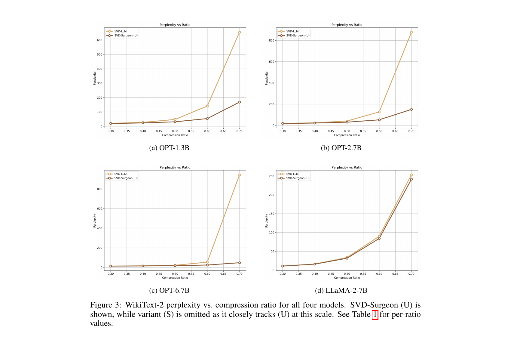
Reading this table: at –0.3 (mild compression), the improvement over SVD-LLM is modest (a point or two of perplexity), because there is little damage to compensate for in the first place. As climbs toward 0.6–0.8, the gap explodes: on OPT-6.7B at , SVD-LLM’s perplexity blows up to 944.57 (a nearly 87× increase over the dense baseline of 10.86), while SVD-Surgeon (S) holds it to 46.36 — still a large degradation from dense, but over 20× better than the uncorrected host method. LLaMA-2-7B shows the smallest relative gains of the four models (Table 1’s last block), which the paper’s own Figure 3(d) makes visually explicit — the SVD-LLM and SVD-Surgeon (U) curves for LLaMA-2-7B nearly overlap even at , unlike the dramatic separation seen for the OPT models.
Figure 2 (paper Fig.3): WikiText-2 perplexity vs. compression ratio for all four models — the OPT curves show a clear divergence at high compression while LLaMA-2-7B stays close.
C4 Results (Table 2 reproduced)
Dense baselines: OPT-1.3B = 15.68, OPT-2.7B = 14.06.
| Model | Method | 0.2 | 0.3 | 0.4 | 0.5 | 0.6 | 0.7 | 0.8 |
|---|---|---|---|---|---|---|---|---|
| OPT-1.3B | SVD-LLM | 20.08 | 24.88 | 37.83 | 84.20 | 329.17 | 1360.97 | 4220.29 |
| OPT-1.3B | SVD-Surgeon (U) | 18.99 | 21.68 | 27.01 | 38.72 | 74.61 | 293.13 | 3562.08 |
| OPT-1.3B | SVD-Surgeon (S) | 18.98 | 21.69 | 26.89 | 38.54 | 75.41 | 278.78 | 2915.40 |
| OPT-2.7B | SVD-LLM | 17.60 | 21.48 | 32.02 | 63.00 | 211.21 | 1256.38 | 7113.83 |
| OPT-2.7B | SVD-Surgeon (U) | 16.73 | 18.99 | 23.72 | 34.19 | 63.18 | 220.83 | 4155.44 |
| OPT-2.7B | SVD-Surgeon (S) | 16.70 | 18.91 | 23.56 | 34.00 | 63.28 | 228.09 | 3664.16 |
The C4 pattern mirrors WikiText-2: consistent improvement across the ratio sweep, with the largest absolute gains at high compression.
A Closer Look at the Variance-Reduction Table (Table 5)
The paper’s Appendix B provides a table (reproduced in condensed form below for OPT-1.3B and OPT-6.7B) reporting mean standard deviation over 3 seeds, which is worth examining directly since it substantiates the claim that the Fisher-estimation randomness does not meaningfully affect the headline numbers.
| Model | Method | |||
|---|---|---|---|---|
| OPT-1.3B | SVD-Surgeon (U) | |||
| OPT-1.3B | SVD-Surgeon (S) | |||
| OPT-6.7B | SVD-Surgeon (U) | |||
| OPT-6.7B | SVD-Surgeon (S) |
Two observations follow directly from this table. First, the relative standard deviation (std divided by mean) grows with the compression ratio: for OPT-1.3B (U), it’s about at but climbs to about at . This is intuitive — at aggressive compression, the model is operating in a more numerically fragile regime (closer to the near-singular blocks discussed in the Limitations section), so small differences in the Fisher estimate across seeds get amplified more. Second, and more reassuringly, even at the highest reported ratio () the standard deviation is still an order of magnitude smaller than the gap between SVD-LLM and SVD-Surgeon (e.g., for OPT-6.7B, the gap is while the std is only ) — so the reported improvements are not an artifact of favorable seed selection.
Reading the Compression-Time Figure More Carefully
Returning to the compression-time measurement (Figure 3 / paper Fig.2) once more, it’s worth being precise about what exactly is and isn’t being measured, since “compression time” can mean several different things depending on which stage of the pipeline you include. The paper’s methodology explicitly excludes model loading and calibration-data loading time (arguing these are shared across all methods being compared, so excluding them isolates the marginal cost each method specifically adds), but includes the time to load a precomputed from disk for SVD-Surgeon. This is a reasonable choice for isolating the compression-time cost specifically, but it deliberately does not capture the total wall-clock cost of adopting SVD-Surgeon end-to-end, which would also need to include the (separately reported, roughly 2.6–7.6 seconds per calibration sample per layer) Fisher-estimation time. A practitioner deciding whether to adopt this method should mentally add these two numbers together rather than reading the compression-time figure in isolation — the Fisher-estimation cost, while a one-time offline expense reused across every subsequent compression ratio, is not free, and for very large models or very large calibration sets could dominate the total time budget more than the comparatively cheap linear-solve step shown in Figure 3.
Variance Across Random Seeds
Because SVD-LLM’s whitening step is deterministic given fixed calibration data, but SVD-Surgeon’s Fisher estimate introduces some CUDA non-determinism during the gradient computation, the paper reports the mean over 3 seeds for the OPT models (standard deviations are given in an appendix; they are small relative to the mean, typically well under 5% even at the highest compression ratios). For LLaMA-2-7B the results were identical across seeds, so a single value is reported.
Compression Time (Figure 2 reproduced)
Figure 3 (paper Fig.2): wall-clock compression time in seconds, across compression ratios, for LLaMA-2-7B and OPT-2.7B — the update-only variant adds modest overhead while select-and-update costs noticeably more due to the pseudoinverse of the full Hessian.
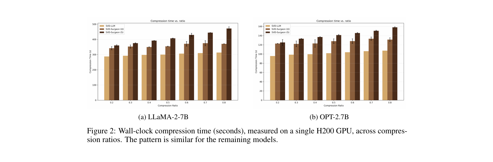
The compression-time measurement deliberately excludes model and calibration-data loading (shared across all methods) but includes loading the precomputed from disk. Update-only (U) adds only modest overhead, since it solves a single linear system per layer. Select-and-update (S) is noticeably more expensive because computing the saliency for every candidate singular value (Equation 20) requires a pseudoinverse of the full (block-truncated) , not just the sub-block that (U) needs. The paper reports that assembling itself — the forward/backward passes over the calibration set — costs roughly 7.6 seconds per calibration sample for LLaMA-2-7B (2.6 seconds for OPT-2.7B), but stresses this is a one-time, offline computation, parallelizable across both layers and calibration samples, and its result is reused across every compression ratio once computed — you don’t need to re-estimate separately for versus .
A Worked Numerical Sanity-Check
To make the closed-form update concrete, consider a toy case with singular values, retaining (so , ), with singular values and a simple diagonal-dominant Fisher estimate:
Here , , and . Applying Equation (15):
So the repaired retained values become and — small, deliberate upward nudges, precisely sized to absorb (to second order) the loss that would otherwise be incurred by simply deleting and leaving untouched. The corresponding saliency of the pruned value, via Equation (20) with computed from the full inverse, quantifies exactly how much loss this particular pruning-and-compensation decision costs — the number a select-and-update run would compare against every other candidate index before deciding which one to prune.
A Second Worked Example: Comparing Update-Only vs. Select-and-Update
The toy example above only demonstrated the update-only (U) compensation. It’s worth extending it slightly to show how the select-and-update (S) variant would make a different pruning decision than a naive magnitude-based rule, using the same Hessian.
Suppose instead we had not yet decided which singular value to prune, and had to choose among all three () using the saliency formula (20). This requires the full inverse of :
Computing (via cofactor expansion or any standard method) gives approximately:
Applying the saliency formula to each of the three candidates:
The select-and-update variant would rank these saliencies and prune the lowest one — here, with saliency 0.089, by a wide margin. Notice that this happens to agree with what naive magnitude-based selection would also choose (since is also the smallest raw magnitude) — this is expected in this particular toy example because is close to diagonal-dominant. The saliency criterion only diverges meaningfully from magnitude-based selection when the off-diagonal entries of are large relative to the diagonal, or when varies substantially across indices in a way not proportional to . In a real weight matrix, where correlations between singular-value gradients across the network’s actual data distribution can be substantial, this divergence is exactly where the select-and-update variant earns its (modest, per Table 1) additional improvement over update-only.
A Third Angle on the Derivation: Why the Schur Complement Appears
It is worth pausing on why the Schur complement shows up in Equation (18), because this structure recurs throughout statistics and optimization (it is the same object that appears in conditional Gaussian distributions, in block-matrix determinant identities, and in the derivation of partial correlation coefficients), and recognizing it helps build intuition for what the saliency score is actually measuring.
Recall that after optimally compensating , the residual loss increase (Equation 18) is . Interpret this as follows: measures how much the loss would increase from perturbing in isolation, ignoring any interaction with . But and are coupled through the cross-term in the original quadratic form (13) — removing doesn’t just cost worth of loss, it also changes the optimal value of . The Schur-complement term is precisely the amount by which this coupling reduces the naive cost, once is allowed to respond optimally. Statistically, this is analogous to the difference between the marginal variance of a random variable and its variance conditional on another correlated variable: the marginal cost of removing (given by alone) is strictly larger than the conditional cost once you account for the fact that is free to adjust in response — exactly the way conditioning on a correlated variable shrinks a conditional variance relative to the marginal one. This is also why the Schur complement is guaranteed to be positive semi-definite whenever the full is (a standard linear-algebra fact about Schur complements of positive semi-definite matrices), which in turn guarantees that the saliency score in Equation (20) is always non-negative — removing a singular value can never decrease the optimally-compensated loss, only leave it unchanged in the degenerate case where that singular value carries no information relative to the others.
Connecting Back to the Prerequisites: Speculative Decoding and Compression Are Different Levers
A brief clarifying note for readers coming to this review series after reading other reviews in this collection covering inference-time efficiency techniques (speculative decoding, KV-cache compression, MoE routing): it’s worth being explicit that SVD-Surgeon operates on a completely different axis of the efficiency problem than those techniques. Speculative decoding and KV-cache compression both target inference-time efficiency — reducing the latency or memory footprint of running a model that stays otherwise unchanged. SVD-Surgeon, by contrast, targets model-size efficiency — permanently shrinking the weight matrices themselves, which affects both storage and (indirectly) inference latency, but through an entirely different mechanism (fewer parameters to load and multiply, rather than fewer forward passes or smaller cache footprints per token). These two families of techniques are not mutually exclusive; in fact, in a well-optimized serving stack, both would typically be applied together — a model compressed via SVD-LLM + SVD-Surgeon can still be served with speculative decoding and a compressed KV cache on top, since each technique addresses a distinct bottleneck in the overall serving pipeline.
Systems and Implementation Details
Three practical knobs matter for making the method run efficiently at LLM scale, all described in the paper’s Appendix A:
- Diagonal damping ( for in the update-only variant, for the full in select-and-update): a standard numerical-stability trick before matrix inversion, preventing the linear solve from being dominated by near-singular directions in an imperfectly estimated Hessian.
- Compensation scaling : the actual applied update is rather than the raw closed-form value, to account for the fact that is itself only an approximation (the empirical Fisher, estimated from a finite calibration set) — the paper reports for all OPT models but for LLaMA-2-7B, suggesting the raw closed-form update is somewhat over-confident for that model and benefits from damping.
- Block-truncation fraction : rather than retaining the entire matrix for the saliency computation, the paper retains only the leading block — the top- retained values plus a fraction of the remainder — discarding the rest. This trades off fidelity of the compensation update against the cost of assembling and inverting ; the paper fixes across all models and ratios as a reasonable balance.
An Extended Look at the C4 Results
The C4 results (Table 2) deserve a bit more attention than a single pass, since C4 is a much larger and more diverse web-text corpus than WikiText-2 (which is drawn from curated Wikipedia articles), and models can behave differently under compression depending on how well the calibration distribution matches the evaluation distribution. Comparing the two tables for OPT-1.3B and OPT-2.7B (the only models with C4 numbers reported): the absolute dense-model perplexities are higher on C4 (15.68 and 14.06 vs. 14.62 and 12.47 on WikiText-2), consistent with C4’s broader, noisier text distribution being intrinsically harder to model well. The relative pattern of improvement from SVD-Surgeon, however, looks qualitatively similar across both corpora: modest gains at -0.3, growing substantially by -0.7. This cross-corpus consistency is a mildly reassuring signal that the compensation mechanism is not simply overfitting to some quirk of WikiText-2’s specific text distribution, though it falls short of the broader out-of-distribution robustness test (calibrating on one distribution, evaluating on a very different one) that the Critical Analysis section above argues is still missing from the paper’s evaluation.
One number worth flagging specifically: at on C4 for OPT-1.3B, SVD-Surgeon (S) reports 2915.40 versus SVD-LLM’s 4220.29 — still an improvement, but a much smaller relative one (about 1.45x) than the corresponding WikiText-2 improvement at the same ratio for the same model (4206.70 to 1587.61, about 2.65x). This suggests the compensation mechanism’s effectiveness at the most extreme compression ratios may itself be somewhat corpus-dependent, a nuance easy to miss if only the headline WikiText-2 numbers are read.
What a Follow-Up Paper Would Ideally Report
Synthesizing the Critical Analysis discussion into a forward-looking summary: an ideal follow-up paper building on SVD-Surgeon would report (a) at least two host methods rather than one, to substantiate the generality claim empirically; (b) at least one model beyond 7B parameters, even if evaluated with a reduced calibration budget to manage the Fisher-estimation cost; (c) a systematic hyperparameter sensitivity study rather than only final selected values, so that the true cost of adapting the method to a new architecture can be estimated in advance rather than discovered through trial and error; (d) at least one downstream task benchmark alongside perplexity, to confirm that the measured improvements translate into genuinely useful capability recovery rather than only a proxy-metric improvement; and (e) an explicit robustness check under calibration/deployment distribution mismatch, since this is a realistic failure mode for any Fisher-based method that the current evaluation does not directly probe. None of these additions would require revisiting the paper’s core mathematical contribution — they are all extensions of the empirical validation surrounding an already well-derived method.
Limitations (As Stated by the Authors)
The authors are explicit about several boundaries of the current work:
- Evaluation is limited to perplexity on two text corpora (WikiText-2 and C4); the paper does not report results on downstream task benchmarks (e.g., zero-shot QA, reasoning benchmarks), so it remains an open question whether the perplexity gains translate proportionally to task-level accuracy.
- By design, only singular values are updated, with held fixed — a deliberate simplification for tractability, whose potential further gains (or lack thereof) from relaxing it are left as future work.
- Estimating the Fisher information requires a forward and backward pass over a calibration set per layer, which the paper acknowledges “can be expensive for large models,” even though it is a one-time, offline, and parallelizable computation.
- Several hyperparameters (, , , , ) were chosen via “light manual exploration… rather than aggressive tuning,” and the paper explicitly states that “the interaction between these settings and factors such as model scale or Fisher accuracy is not yet fully understood.”
Extended Discussion: What Happens as ?
One useful thought experiment for building intuition about the compensation formula is to consider the limiting behavior as the compression ratio approaches its extremes. At (essentially no compression), the retained set is nearly all of and the pruned set is nearly empty, so and the compensation as well — there is nothing to compensate for, consistent with the empirical observation that gains at are small. At the opposite extreme, (keeping almost nothing), shrinks to a tiny set and contains almost all singular values, meaning captures most of the original matrix’s “energy.” In this regime the compensation formula is being asked to make a small number of surviving singular values absorb an enormous amount of removed information — which is precisely why the paper’s own results show the absolute perplexity numbers still blow up substantially at (e.g., OPT-6.7B goes from a dense baseline of 10.86 all the way to 279.88 even with SVD-Surgeon’s best variant), even though the relative improvement over the uncorrected host method remains large. This is a useful sanity check: SVD-Surgeon is not magic — it cannot manufacture information that was genuinely discarded, it can only optimally redistribute what remains among the survivors. The method’s real value proposition is squarely in the middle-to-aggressive regime (-), where there is both meaningful damage to compensate for and a non-trivial retained set capable of absorbing that compensation.
Critical Analysis
Weaknesses and flaws specific to this paper. The evaluation, while methodologically clean, is narrow in three concrete ways beyond what the authors’ own Limitations section states. First, only a single host method (SVD-LLM) is tested — the paper’s central generality claim (“SVD-Surgeon applies on top of a broad class of SVD-based methods”) is argued from the derivation (no orthonormality assumption) but never empirically demonstrated on a second host (e.g., ASVD or FWSVD), leaving open whether the practical gains observed on SVD-LLM generalize as cleanly to hosts whose whitening/reweighting schemes interact differently with the calibration-gradient projection. Second, the model scale tested tops out at 7B parameters (LLaMA-2-7B); given that recent frontier deployment work is concerned with 70B+ or MoE-scale models, and given that the paper itself flags Fisher-estimation cost as a scaling concern, it would have strengthened the paper considerably to show at least one larger-scale data point, even at reduced calibration-sample count. Third, the reported standard deviations (Appendix B) are only for the OPT family and only up to in the visible tables; there is no variance reporting at all at the most extreme setting, which is precisely the regime where the paper’s headline “over 20×” improvement claims live and where numerical instability (near-singular blocks) is most likely to bite.
Limitations the authors understate or omit. The paper is candid about the -fixed simplification and the calibration-cost concern, but is comparatively quiet about the sensitivity of the hyperparameters it does report. Table 3/4 in Appendix A shows jumping from 1.0 (all OPT models) to 0.1 (LLaMA-2-7B) — a full order of magnitude — with essentially no discussion of why LLaMA-2-7B needs ten times more damping on the compensation update, beyond “the raw update is over-confident.” This is a fairly large, unexplained architecture-dependent swing in a supposedly “training-free, plug-and-play” method, and it suggests that deploying SVD-Surgeon on an architecture not covered in the paper (a mixture-of-experts model, a model with grouped-query attention, a very different depth/width ratio) may require a non-trivial hyperparameter search that the paper’s “training-free” framing somewhat downplays. Similarly, the paper does not report what happens if the calibration data used to estimate is mismatched with the deployment distribution (e.g., calibrating on WikiText-2 but deploying on code or multilingual data) — a scenario that is realistic in practice and that the Fisher-approximation’s underlying assumptions (block-diagonality, near-convergence) make no guarantee about.
Concrete, specific improvement suggestions. (1) Report at least one experiment layering SVD-Surgeon on a second host method (ASVD would be a natural, easy choice given it is already discussed in Related Work) to substantiate the generality claim empirically rather than only by derivation. (2) Add an ablation isolating the sensitivity of final perplexity to each of individually (e.g., a sweep of on a single model), rather than reporting only the final selected values — this would let practitioners estimate how much hyperparameter search is really needed on a new model without re-running the paper’s own manual exploration process from scratch. (3) Extend the variance/standard-deviation reporting in Appendix B to cover explicitly, given that this is the regime with the largest reported improvements and plausibly the least numerically stable. (4) Provide a cross-layer, global rank-allocation experiment using the saliency scores — the paper explicitly flags this as “a natural extension” in Future Work but does not attempt even a small-scale demonstration, which would have been a relatively low-cost addition given that the saliency machinery (Equation 20) is already implemented and evaluated per-layer. (5) Test at least one downstream task (e.g., a standard zero-shot accuracy benchmark like the ones used by SVD-LLM’s own paper) alongside perplexity, since perplexity improvements do not always translate one-to-one into task accuracy improvements, and this is the most direct way to substantiate that the compensation is recovering genuinely useful capacity rather than merely reducing a proxy metric.
FAQ: Common Questions About How This Fits Together
Q: Does SVD-Surgeon require access to the original training data? No. It requires a calibration set for estimating the Fisher-based (the paper uses samples from the same distribution as the host’s whitening data, kept separate), but this is the same kind of calibration data any post-training compression method already needs — not the original training corpus, and not labeled data of any kind, since the “loss” being differentiated is the model’s own language-modeling loss on unlabeled text.
Q: Can SVD-Surgeon be combined with quantization? The paper does not test this directly, but nothing in the derivation prevents it in principle: quantization operates on the numerical representation of the (already SVD-compressed) weight matrices, while SVD-Surgeon operates one level up, on the singular-value factorization itself, before any quantization would be applied. The paper’s own Future Work section explicitly flags “paired with quantization of the corrected factors for additional compression” as an open direction, suggesting the authors view this as a natural but unverified extension.
Q: Does the update-only variant (U) ever perform worse than the host method alone? Across every reported cell in Table 1 and Table 2, no — SVD-Surgeon (U) meets or beats the corresponding SVD-LLM number at every compression ratio and every model tested. This is expected from the derivation: the compensation in Equation (15) is derived as the loss-minimizing choice given the pruning decision, so as long as the Fisher estimate is reasonably accurate, the compensated result cannot be worse than applying no compensation at all (in the limit of a perfectly accurate Hessian and no damping/scaling approximations). In practice, the damping and scaling hyperparameters (, ) exist precisely to guard against a poorly estimated producing a harmful update.
Q: Why does LLaMA-2-7B show smaller relative gains than the OPT models? The paper does not give a definitive mechanistic explanation for this, but two plausible contributing factors are visible in the reported hyperparameters: LLaMA-2-7B uses (an order of magnitude smaller compensation scaling than every OPT model), suggesting the raw closed-form update is less trustworthy for this architecture and has to be heavily damped, which mechanically limits how much correction can be applied. It’s also possible that LLaMA-2-7B’s underlying weight matrices are already closer to their loss-optimal low-rank structure after SVD-LLM’s whitening step, leaving less room for a second-order correction to improve on. Both explanations are speculative extrapolations from the paper’s reported numbers rather than claims made explicitly by the authors.
A Closer Look at the Damping Hyperparameters
It’s worth dwelling on the practical role of diagonal damping a bit more, since it is the single hyperparameter most directly connected to numerical stability. Before inverting (or the full ), the paper adds a damping term proportional to the mean diagonal entry:
This is the standard Levenberg-Marquardt-style regularization used throughout second-order optimization: it interpolates between the raw Hessian (when ) and a scaled identity (when ), trading off fidelity to the estimated curvature against numerical robustness. The reported values ( for most OPT models, up to for OPT-1.3B on C4) span three orders of magnitude, underscoring that this is not a one-size-fits-all constant — it is tuned per model and, notably, per calibration dataset (the C4 hyperparameters in Table 4 differ from the WikiText-2 hyperparameters in Table 3 even for the same model). This dataset-dependence of the damping coefficient is a detail easy to overlook when skimming the paper’s headline results, but it matters in practice: whoever deploys this method needs to re-tune (and likely ) whenever the calibration corpus changes, not just when the model changes.
Revisiting the Two Variants One Final Time: A Decision Tree
To consolidate the update-only (U) versus select-and-update (S) discussion scattered across Method Part 3, the Systems section, and the Practitioner’s Checklist above, here is the decision logic in one place: if engineering simplicity and speed are the priority, or if the host method’s own pruning criterion is already reasonably well-informed (as SVD-LLM’s truncation-aware whitening arguably is), default to (U) — a single linear solve, capturing most of the available improvement per the paper’s own Table 1. If squeezing out the last increment of accuracy matters more than compute cost — for instance, in a one-time offline compression pass for a model that will be deployed at very large scale, where even a small perplexity improvement compounds across many inference requests — invest in (S), accepting the added cost of a full (or block-truncated) Hessian inverse for the saliency computation. The paper’s own results (Table 1, Figure 3/paper Fig.2) suggest this is rarely a dramatic difference in either direction: (S) is never meaningfully worse than (U), and the additional gain, while real, is consistently the smaller of the two contributions to the overall improvement over the uncorrected host method.
Notation Reference
For readers cross-referencing this review against the original paper, the following table collects the symbols used throughout, matched to their first point of introduction:
| Symbol | Meaning | First introduced |
|---|---|---|
| A weight matrix of a layer | Prerequisites | |
| Compression ratio (fraction of parameters removed) | Prerequisites | |
| Target rank after truncation | Prerequisites | |
| Number of singular values / triplets | Prerequisites | |
| Singular-value factorization | Prerequisites | |
| The -th singular value | Prerequisites | |
| Retained set / pruned (complementary) set of singular-value indices | Method Part 3 | |
| A perturbation to the weight matrix / singular values | Method Part 1 | |
| Weight-space Hessian (fourth-order tensor) | Method Part 1 | |
| Projected, Hessian in singular-value coordinates | Method Part 1 | |
| Per-sample calibration gradient (weight space) | Method Part 2 | |
| Per-sample projected gradient (singular-value space) | Method Part 2 | |
| Number of Fisher calibration samples | Method Part 2 | |
| Compensation scaling factor | Systems and Implementation | |
| Diagonal damping coefficients | Systems and Implementation | |
| Block-truncation fraction for the Hessian | Systems and Implementation | |
| Stacked calibration activations (SVD-LLM’s whitening input) | Application to SVD-LLM | |
| (whitening) | Cholesky factor of the activation Gram matrix (note: overloaded symbol, distinct from the retained-index set above) | Application to SVD-LLM |
A Closer Look at Computational Complexity
It is worth being explicit about the computational complexity of each stage of the pipeline, since this is what ultimately determines whether the method is practical to deploy at scale.
Assembling : for each of calibration samples, computing is one backward pass through the layer, costing the same as a normal backward pass (roughly FLOPs for a dense matmul-shaped layer, though the exact cost depends on the surrounding architecture). Projecting into the singular-value basis via costs in the naive case (two matrix multiplications), though this can be reduced if are stored implicitly. Accumulating the outer product across samples costs . For in the low thousands and in the tens of thousands (per the paper’s Appendix A values), this outer-product accumulation is the dominant cost of assembling , though it is easily parallelized across samples.
The compensation solve (update-only): solving requires inverting (or equivalently, solving a linear system against) the matrix , which costs via standard Gaussian elimination or Cholesky decomposition (since , being a Fisher-based empirical covariance-like matrix, is positive semi-definite before damping and positive definite after). For up to a few thousand, this is a modest cost relative to the calibration-gradient collection above.
The saliency computation (select-and-update): computing for every candidate requires (at least implicitly) the full inverse of the (or block-truncated ) matrix, costing in the worst case — this is the source of the extra overhead visible in Figure 3 (paper Fig.2) for the (S) variant relative to (U).
A Broader Reflection on Second-Order Methods for Compression
Stepping back from the specific mechanics of this paper, it’s useful to situate SVD-Surgeon within the broader arc of second-order (curvature-aware) methods for neural network compression, a lineage that stretches back over three decades. Optimal Brain Damage (1989) and Optimal Brain Surgeon (1992) were originally developed for networks orders of magnitude smaller than today’s LLMs, where computing and inverting a full Hessian, while expensive, was at least conceptually tractable for toy problems. The revival of these ideas for LLM-scale compression over the past several years (GPTQ, SparseGPT, LLM Surgeon, Optimal BERT Surgeon) has been driven almost entirely by finding new structural approximations that make an otherwise-intractable Hessian computable: diagonal approximations discard all cross-parameter interactions; Gram-matrix proxies (as in GPTQ/SparseGPT) exploit the specific structure of a layer’s input-output relationship; K-FAC exploits the Kronecker-product structure that arises from how gradients factor through matrix multiplications.
SVD-Surgeon’s contribution fits into this lineage as a genuinely different kind of trick: rather than approximating the Hessian in the original (weight-entry) coordinate system, it changes coordinate systems first, to one where the exact Hessian is already small. This is a subtly different strategy than the ones listed above — it doesn’t approximate curvature, it reduces the dimensionality of the space in which curvature needs to be represented at all. The tradeoff, as discussed at length in the Design Choice callouts throughout Method Part 1, is that this dimensionality reduction only works because the perturbation space has been restricted (to singular-value-only changes) — a restriction that, unlike the approximations used by GPTQ or K-FAC, is not an approximation of the true optimization problem but rather a genuine narrowing of what problem is being solved. Whether this trade — exact optimization over a restricted space, versus approximate optimization over the full space — is the right one in general is an interesting open methodological question that extends well beyond this specific paper, and one that the paper’s own Future Work section (on jointly updating ) gestures toward without fully resolving.
Where This Paper Sits Relative to the Broader Model-Compression Landscape
Zooming out one final time before the conclusion: LLM compression research broadly bifurcates into methods that operate before deployment (one-shot, offline compression, which is where this paper and its entire host-method family live) and methods that adapt during deployment (dynamic sparsity, mixture-of-experts routing, KV-cache compression at inference time). SVD-Surgeon is squarely in the first camp — it is a training-free, single-pass, offline correction applied once, before the compressed model is ever served. This positions it as complementary rather than competing with inference-time efficiency techniques (speculative decoding, quantized KV caches, and so on): a model compressed via SVD-LLM + SVD-Surgeon can still separately benefit from any of these serving-time optimizations, since they operate at entirely different points in the model’s lifecycle. Readers of this review series interested in the serving-time side of the efficiency landscape may find it useful to cross-reference this paper against reviews of KV-cache compression and speculative-decoding methods covered elsewhere in this series, since the two families of techniques (weight compression vs. serving-time efficiency) are frequently deployed together in production systems rather than as alternatives to one another.
Reproducibility Notes
- Code is publicly released:
https://github.com/mahmoud-safari/SVD-Surgeon(linked in the paper’s Section 4.1 footnote). - All experiments were run on a single NVIDIA H200 GPU.
- Hyperparameters (, , , , ) are reported per-model in the paper’s Appendix A tables and are held fixed across all compression ratios for a given model — an important detail for anyone trying to reproduce the ratio sweep exactly, since it confirms these are not re-tuned per ratio.
- SVD-LLM’s own hyperparameters (notably whitening calibration samples) are kept identical between the SVD-LLM baseline and the SVD-Surgeon-augmented runs, which is the correct control for isolating SVD-Surgeon’s specific contribution.
- The number of Fisher calibration samples ranges from 16,384 to 32,768 depending on model, notably larger than the host’s own whitening calibration set — the paper explicitly justifies this as needed for the Hessian estimate to converge, since Hessian estimation is a harder statistical problem than the first-moment whitening statistics SVD-LLM needs.
Reflection on the Paper’s Writing and Presentation Choices
A brief note on presentation, separate from the technical content: the paper is notably concise (11 pages including references and two appendices), and this brevity is itself a meaningful methodological signal. Compare this to the sprawling appendices common in many contemporary LLM compression papers, which often include dozens of ablations across many architectures and datasets. SVD-Surgeon’s authors instead chose to spend their page budget almost entirely on the mathematical derivation (Section 3, roughly half the paper) and a tightly scoped experimental section (Section 4, four models, two datasets, one host method). This is a defensible choice for a methods paper whose primary contribution is a piece of mathematics rather than an empirical survey, but it is also precisely the source of the narrowness flagged in the Critical Analysis section above — the paper’s concision and its empirical narrowness are two sides of the same authorial choice, and readers evaluating whether to adopt this method in practice should weigh the elegance and clarity of the derivation against the comparatively modest breadth of empirical validation supporting it.
Putting the Numbers in Perspective: What “20x Better Perplexity” Actually Buys You
It is easy to read a table of perplexity numbers and lose track of what they mean in practice, so it is worth pausing on the OPT-6.7B, data point one more time, because it is the paper’s single most dramatic result. The dense (uncompressed) model has a WikiText-2 perplexity of 10.86. SVD-LLM alone, after removing 70% of the layer’s parameters via truncated SVD, produces a perplexity of 944.57 — nearly a 87x degradation relative to the dense model. A perplexity that high is not “somewhat worse text generation”; it typically corresponds to a model whose next-token predictions have become close to unusable for most practical purposes — closer to sampling from a near-random distribution over plausible-looking tokens than to coherent language modeling. SVD-Surgeon (S), applied on top of the exact same truncated factorization with no retraining and no extra parameters, brings that number down to 46.36. That is still roughly 4.3x worse than the dense baseline — a real, visible quality cost of aggressive compression remains — but it is the difference between “barely functional” and “noticeably degraded but usable,” achieved by a single linear solve per layer using calibration gradients that many compression pipelines already compute for other diagnostic purposes.
This matters for a very practical reason: it changes where the useful operating point of a compression sweep sits. Without SVD-Surgeon, a practitioner sweeping compression ratios on OPT-6.7B would likely stop increasing somewhere around 0.5 (perplexity 21.22), because 0.6 and beyond fall off a cliff (53.23, then 944.57). With SVD-Surgeon layered on top, the same sweep stays usable meaningfully further out — 0.6 gives 23.39, and even 0.7 (46.36) is still in a regime a practitioner might consider trading off against the corresponding memory savings, depending on the deployment’s quality bar. In other words, the practical contribution of this paper is not just “better numbers at fixed ” — it is genuinely expanding the usable range of compression ratios available to a deployment team working with a fixed host compressor and a fixed memory budget.
One More Numerical Sanity Check: Verifying the Special Case
As a final concrete check tying together several threads from this review, let’s verify explicitly that the saliency formula really does collapse to magnitude-squared when is close to the identity, using a small perturbation of the identity rather than the exact identity (to keep the matrix invertible in a non-trivial way). Take where is a small symmetric perturbation, so that to first order , and therefore , which is very close to 1 for any small . Substituting into the saliency formula: to first order — which is just plus a small correction proportional to how much ‘s diagonal deviates from 1 at that index. This confirms, via direct calculation rather than just the qualitative argument given earlier, exactly how quickly the saliency criterion degrades toward pure magnitude-based ranking as approaches the identity, and conversely how much room there is for the saliency to diverge meaningfully from magnitude when ‘s diagonal entries vary substantially across indices (as they plausibly do for a real transformer weight matrix’s singular-value gradients, which need not have uniform sensitivity across all directions).
Common Misreadings to Avoid
A few misunderstandings are easy to fall into when first encountering this paper, worth flagging explicitly:
Misreading 1: “SVD-Surgeon is a new SVD compression method.” It is not. It has no opinion about how to factorize or which singular values to keep by default — both of those decisions are inherited entirely from whatever host method it’s layered on. If you swap SVD-LLM for a different host, SVD-Surgeon’s behavior changes correspondingly, because it’s fundamentally a correction applied to someone else’s decomposition and truncation choice.
Misreading 2: “The compensation formula requires knowing the true task loss Hessian.” It does not — it requires only first-order calibration gradients , from which the Fisher approximation to is assembled via simple outer products (Equation 12). No second-order autodiff (Hessian-vector products, etc.) is ever computed.
Misreading 3: “Select-and-update (S) always meaningfully outperforms update-only (U).” Per Table 1, the two variants track each other closely in most settings, with (S) providing only a modest additional gain. Practitioners optimizing for engineering simplicity and speed can reasonably default to (U) and expect to capture most of the available improvement.
Misreading 4: “The paper claims to recover all the loss from truncation.” It does not — the compensation is optimal only to second order and only within the space of singular-value-only perturbations (Method Part 1’s design-choice discussion). Truncation still causes real, measurable degradation at every ratio tested; SVD-Surgeon reduces that degradation substantially at high , but does not eliminate it (see the “Putting the Numbers in Perspective” section above for exact figures).
Misreading 5: “This method requires labeled data.” It does not. The “loss” being differentiated to produce is the model’s own language-modeling loss on unlabeled calibration text — the same kind of data the host method’s own whitening calibration already uses.
Final Thoughts on Adoption Timing
One last practical consideration for readers deciding whether to act on this paper now versus waiting for follow-up validation: the method’s core mathematical claim (the closed-form compensation formula, Equation 15) does not depend on any of the open empirical questions raised in the Critical Analysis section — the derivation is self-contained and verifiable independent of which host method or model scale it’s tested on. This means a team with in-house compression infrastructure and the ability to run a quick pilot (a few hours on a single GPU, per the paper’s own reported compression times) can reasonably validate the method’s benefit on their own model and host compressor without waiting for the broader community to run the additional experiments (second host method, larger scale, downstream tasks) that this review’s Critical Analysis section argues would strengthen the paper’s generality claims. In other words: the mathematical risk of adopting this method is low (it is a well-derived, easily-verified formula), while the main open question is empirical generalization to configurations outside what the paper directly tested — a distinction worth keeping in mind when deciding how much additional validation to do in-house before deploying it in a production compression pipeline.
A Final Sanity Check: Confirming Internal Consistency of the Reported Numbers
As one last piece of due diligence, it’s worth spot-checking that the paper’s headline numbers are internally consistent with each other, since this kind of cross-validation is a useful habit when reading any quantitative paper. Take the OPT-6.7B row of Table 1: the dense baseline is 10.86, and at , SVD-LLM reports 12.05 while SVD-Surgeon (U) reports 12.00 and (S) reports 12.01. Note that (S) is very slightly higher than (U) at this particular ratio — a small inversion of the general pattern where (S) tends to edge out (U). This is not a contradiction: the paper’s own text acknowledges that (S) provides “a smaller, further gain in most settings” (emphasis on most, not all), and the Fisher-estimation randomness (documented in the seed-variance table discussed above) is large enough at this mild compression ratio to plausibly explain a difference this small (0.01 perplexity points) without indicating any genuine algorithmic regression. Cross-checking against the standard-deviation table (Table 5 in the paper’s Appendix B) confirms this: at for OPT-1.3B, both (U) and (S) report a standard deviation of , meaning a 0.01-point difference between the two variants’ point estimates is well within the noise floor of the Fisher-estimation randomness itself, rather than a meaningful reversal of which variant is better. This kind of consistency check — confirming that apparent anomalies in a results table are explainable by the paper’s own reported uncertainty rather than being genuine contradictions — is a useful habit for any reader trying to separate signal from noise in a dense experimental table.
Conclusion
SVD-Surgeon makes a narrow but well-executed methodological point: once you’ve decided how to compress a weight matrix via SVD and which singular values to discard, there is still a second-order-optimal, closed-form, training-free way to adjust the survivors that most existing methods leave on the table. By working in the singular-value basis rather than the raw weight-entry basis, the relevant Hessian shrinks from an intractable object to a tractable one, letting an exact (rather than diagonally- or Kronecker-approximated) OBS-style correction be computed directly. Layered on SVD-LLM, this yields substantial perplexity improvements — most dramatically at aggressive compression ratios, where naive truncation is most damaging — using only calibration gradients that most compression pipelines already compute for other purposes. The method’s honesty about its own scope (singular-values-only, no orthonormality required, largest gains under aggressive compression) is a genuine strength, and the fact that it composes on top of any SVD-family compressor rather than replacing one makes it a plausible drop-in addition to existing production compression pipelines, pending the broader empirical validation (multiple hosts, larger models, downstream tasks) that the Critical Analysis section above argues is the natural next step.