PHOENIX: Recovering LLM Training in 40 Seconds Instead of Restarting the Whole Job

Review date: 2026-07-23 Review author: Zhongzhu Zhou Paper reviewed: PHOENIX: Resilient LLM Training with Hot-Swapping via Zero-Overhead Checkpoint Paper authors: Haotian Xie, Junlin Chen, Mingkai Zheng, Lishan Yang, Zhao Zhang (Rutgers University, George Mason University) arXiv: 2607.01646 Status: Preprint, July 2026

Short Answer

Training a large language model on thousands of GPUs for months is, statistically speaking, an exercise in failure management. Hardware breaks constantly at that scale — a report from a 32K-GPU pretraining deployment counted 678 unexpected interruptions, with memory faults, PCIe errors, and NCCL timeouts alone responsible for half of them. The standard defense, periodic checkpoint-restart, pays a double tax: it slows down every normal step a little bit to write checkpoints, and when a failure actually happens, the entire job has to stop, reload the last checkpoint from disk, and re-execute all the training steps that happened after that checkpoint was taken. On a cluster running at O(100K) GPUs, a real-world measurement cited in this paper puts synchronous recovery stalls at roughly 10 minutes and the expected lost-work replay at up to 16.7 minutes — for a single failure, and failures there occur roughly every 18 minutes. PHOENIX attacks both halves of that cost simultaneously. Instead of periodically writing a checkpoint to disk, it continuously keeps a recoverable copy of every rank’s optimizer state in the memory of a neighboring machine, overlapped so tightly with normal computation that it introduces no measurable slowdown (the paper’s headline claim: literally zero overhead in the failure-free case, verified from 8 to 512 GPUs and from 0.6B to 65B parameters). When a node permanently dies, PHOENIX does not restart the job. It treats the failure as a topology repair problem: attach a spare node, rebuild the communication groups, restore the missing shards from the in-memory replicas held by peers, and resume training from the last completed step — no filesystem I/O, no full torch.distributed re-initialization, no replay of more than a single training step. Measured hot-swap recovery completes in under 40 seconds across all tested scales, an 18.8× reduction in real recovery time compared to checkpoint-restart in the paper’s Monte Carlo failure-injection experiment.

Prerequisites

Before diving into PHOENIX’s design, it helps to have a working mental model of three things: how large-scale LLM training is actually parallelized across GPUs, what a “checkpoint” really contains and costs, and what actually breaks at scale (and how systems classify those breakages). If you already know 3D parallelism and checkpoint-restart cold, you can skip to Disruption Cost Modeling.

How LLM training is spread across a cluster

A modern LLM does not fit on one GPU, and even if it did, training it would take too long on one GPU. So training frameworks split the work across many GPUs using several orthogonal parallelism strategies simultaneously — this combination is usually called 3D parallelism (or with sequence parallelism added, 4D):

• Data parallelism (DP). The simplest form: replicate the entire model on every GPU (or every group of GPUs), and give each replica a different slice of the training batch. After each replica computes its own gradients, all replicas synchronize (all-reduce) so they end up with identical gradients before updating. If you have $D$ data-parallel replicas, you have $D$ full copies of the model conceptually, and the natural “unit of redundancy” is: every other DP replica already has a full copy of the model parameters (though usually not of the sharded optimizer state — more on that below).
• Tensor parallelism (TP). Split individual weight matrices (e.g., in the attention and MLP blocks) within a layer across multiple GPUs, so each GPU holds a slice of every matrix. This requires GPUs to talk to each other on nearly every forward/backward computation (fast interconnect required — this is why TP groups are typically confined to a single node with NVLink).
• Pipeline parallelism (PP). Split the model by layer into a sequence of pipeline stages, each stage living on a different GPU or group of GPUs. A minibatch is chopped into microbatches that flow through the stages like an assembly line, with “bubbles” (idle time) at the start and end of each pipeline round because stage $i+1$ can’t start until stage $i$ finishes the first microbatch.
• Sequence parallelism. A newer fourth axis that partitions the sequence dimension of the query/key/value tensors, letting a single sample’s very long context be split across GPUs (ring attention is the most memory-efficient variant of this, using an outer loop over query blocks and an inner loop over key-value blocks).

A GPU’s logical coordinate in this scheme is a tuple like (DP rank, PP stage, TP rank) [sequence-parallel rank too, if used]. This coordinate matters a great deal for PHOENIX, because it determines exactly which other GPUs hold information that could reconstruct a failed GPU’s state.

What a checkpoint actually contains, and why the optimizer state is the expensive/painful part

When people say “checkpoint,” they usually mean saving enough state to resume training bit-for-bit (or close to it) from where you stopped. For a model trained with the ubiquitous Adam optimizer, “enough state” is more than just the model weights:

• Model parameters — the weights themselves, sharded across GPUs according to the parallelism scheme above.
• Optimizer state — for Adam, this is the first moment ($m$, the running mean of gradients) and second moment ($v$, the running mean of squared gradients) per parameter. In full precision (FP32), this alone can be 2× the size of the parameters, and combined with the FP32 master copy of the weights (kept even if forward/backward run in BF16/FP16), the optimizer-state-plus-master-copy footprint can dwarf the “visible” model size.
• Metadata — the current step index, RNG states (needed for reproducible data shuffling / dropout), and the parallelism configuration itself.

Distributed optimizers such as ZeRO (Zero Redundancy Optimizer) don’t replicate this optimizer state across every data-parallel replica; instead they shard it, so each data-parallel rank only owns and updates $1/D$ of the optimizer state, then all-gathers the pieces it needs. This is a huge memory win, but it has an important consequence for fault tolerance: if one node holding a shard of the optimizer state dies, that piece of the optimizer state is genuinely gone — no other single node has a full copy of it, unlike the model parameters, which (under most 3D-parallel layouts) are replicated identically across every DP peer at the same (PP, TP) coordinate. This asymmetry — parameters are naturally redundant across DP replicas, optimizer state is naturally not — is one of PHOENIX’s key design levers, and we’ll come back to it.

The traditional answer: checkpoint-restart, and what it costs

The dominant fault-tolerance strategy in production LLM training, going back to frameworks like Megatron-LM, is straightforward: every $K$ steps (commonly on the order of hundreds to a thousand), write a full checkpoint of parameters, optimizer state, and metadata to persistent storage (a parallel filesystem). If a failure happens, the entire job is torn down, a new job is launched, every process re-initializes torch.distributed process groups from scratch, the latest checkpoint is read back from disk, and training resumes from that last checkpointed step — re-executing (and therefore re-computing, wasting) every step that happened between the checkpoint and the failure.

This strategy has two distinct costs, and it is worth being precise about which is which, because PHOENIX’s whole pitch is attacking both simultaneously rather than trading one for the other (which is what most prior work does):

1. Error-free overhead: the cost paid on every step (or every $K$ steps), purely to maintain the ability to recover — I/O time to write the checkpoint, and any synchronization needed to make the checkpoint consistent.
2. Recovery cost: the cost paid only when a failure happens — job restart latency (re-initializing distributed process groups, reading the checkpoint from disk, verifying consistency) plus replay cost, the wasted recomputation of every step since the last checkpoint.

There is an unavoidable-seeming tension here: checkpoint more often (smaller $K$) and you reduce the replay cost per failure, but you pay the I/O overhead more often too. Checkpoint less often (larger $K$) and error-free overhead shrinks, but replay cost balloons. Figure 1 in the paper visualizes exactly this landscape, plotting a menu of prior systems along a Pareto frontier between “error-free overhead” (x-axis) and “recovery overhead” (y-axis) — traditional checkpoint-restart methods (Varuna, DataStates, ByteCheckpoint, TRANSOM) sit at the low-overhead / high-recovery-cost end; elastic reconfiguration methods (Oobleck, Parcae, EasyScale, DLRover) and redundant-computation methods (Bamboo) sit toward the other end, tolerating failures by keeping extra live compute redundancy or dynamically reshaping the parallel layout, at the cost of degraded per-step throughput even when nothing has failed.

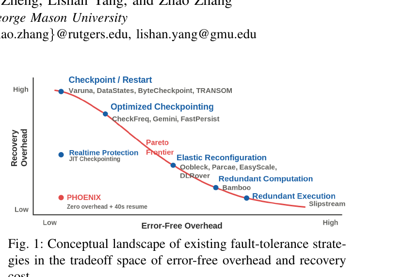
PHOENIX’s claim, visualized as the red dot sitting off the Pareto frontier in Figure 1, is that this tradeoff is not actually fundamental — it is an artifact of how prior systems protect state (persistent, on-disk, periodic checkpoints) and how they recover (full job restart). Change both of those choices, and you can get both benefits at once.

Faults, errors, and failures — a quick taxonomy

The paper (following standard dependability terminology) distinguishes three linked concepts. A fault is a physical root cause — a cosmic ray flipping a bit in DRAM, a degraded PCIe link, a GPU losing ECC integrity. When a fault’s effect reaches the software level and becomes visible to a running program, it becomes an error. An error can then propagate to one of three outcomes: (1) no observable effect, (2) silent data corruption — the program keeps running but produces wrong results without crashing (the scariest category, since prior work has shown it can silently alter trained model parameters), or (3) a failure — a visible crash, hang, or otherwise unresponsive process. PHOENIX is explicitly scoped to failures of category (3): node crashes, GPU errors that make a device unusable, communication timeouts, and similar detectable events. Silent data corruption and software bugs are explicitly called out of scope — handled, if at all, by a separate “external fallback mechanism,” not by PHOENIX itself. Keep this scoping in mind; it matters for the critical-analysis section later.

The Cost of a Failure: A Simple Queueing-Style Model

Before presenting the system, the paper builds a small analytical model of “how bad is a failure, really,” which is worth walking through carefully because it is the quantitative backbone that motivates every design decision that follows, and because the same model is later used (Section VII-C) to compute the paper’s headline 18.8× number.

Modeling checkpoint-restart’s disruption

Define $t_\text{step}$ as the (roughly constant) time for one training step, and suppose checkpoints are written every $K$ steps. If a failure occurs at a uniformly random point between two checkpoints, the number of steps that must be replayed, $R$, has expectation

$$\mathbb{E}[R] \approx \frac{K-1}{2} \tag{1}$$

under a uniform-failure approximation (the failure is equally likely to land anywhere in the $K$-step window). The paper notes real failure processes may be bursty rather than uniform, and offers the more general empirical form $\mathbb{E}[R] = \sum_r r \cdot \Pr(R=r)$ using an empirical replay distribution derived from failure traces, but the uniform approximation is what’s used numerically later, because $(K-1)/2$ is a clean closed form and the bursty correction only matters if you have detailed empirical failure traces (most readers won’t, so the uniform version is the practically useful one).

The total expected disruption per failure event under checkpoint-restart bundles three costs together:

$$\mathbb{E}[C_\text{ckpt}] = C_\text{overhead}^\text{ckpt} + \mathbb{E}[T_\text{restart}] + t_\text{step} \cdot \mathbb{E}[R] \tag{2}$$

Reading this term by term: $C_\text{overhead}^\text{ckpt}$ is the per-checkpoint I/O and synchronization cost paid on the error-free path (this is the “tax” side of the tradeoff — note it’s written here as a per-failure quantity for consistency with the other terms, effectively amortized/attributed cost); $\mathbb{E}[T_\text{restart}]$ is the wall-clock time to tear down and restart the distributed job and reload the checkpoint from disk; and $t_\text{step}\cdot\mathbb{E}[R]$ is the wasted recomputation for the steps that happened after the last checkpoint and were never persisted. The paper explicitly treats this replay time as wasted work, “even though it is re-executed as part of resumed training” — i.e., it’s genuine lost productivity, not merely accounting overhead, because the GPU-hours spent recomputing steps 1..R the second time produce zero additional training progress beyond what was already achieved before the failure.

From per-failure cost to system-wide training efficiency

To turn a per-failure cost into a statement about overall training efficiency, the paper brings in the system-level failure rate via mean time to failure (MTTF). Let $\text{MTTF}_\text{sys}$ be the average time between failures at the whole-system scale, and define the failure rate $\lambda = 1/\text{MTTF}_\text{sys}$. Then the expected disruption per unit time is

$$\mathbb{E}[C_\text{rate}] = \lambda \cdot \mathbb{E}[C_\text{ckpt}] \tag{3}$$

— i.e., you pay the expected per-failure disruption cost $\mathbb{E}[C_\text{ckpt}]$ once every $\text{MTTF}_\text{sys}$ time units on average, so amortized over time you’re paying it at rate $\lambda$. Modeling training as alternating between failure-free intervals of expected length $\text{MTTF}_\text{sys}$ and disruption intervals of expected length $\mathbb{E}[C_\text{ckpt}]$ gives an effective training efficiency

$$\eta \approx \frac{\text{MTTF}_\text{sys}}{\text{MTTF}_\text{sys} + \mathbb{E}[C_\text{ckpt}]} \tag{4}$$

which is the fraction of wall-clock time actually spent making forward training progress rather than recovering. This is a textbook renewal-process approximation (up-time divided by up-time-plus-down-time), and its key qualitative implication is: as system scale grows, $\text{MTTF}_\text{sys}$ shrinks (more failure-prone components means failures happen more often), which amplifies the impact of $\mathbb{E}[C_\text{ckpt}]$ on overall efficiency — the bigger your cluster, the more a slow, replay-heavy recovery mechanism actively hurts you, which is precisely the argument for why fault tolerance design matters more, not less, as training scales up.

The paper grounds this with a concrete number pulled from a cited large-scale deployment study (FT-HSDP, cited as reporting statistics from a real ~100K-GPU training run): at O(100K) GPUs, failures occur roughly once every 18 minutes, synchronous recovery stalls the whole job for about 10 minutes, and checkpoints are commonly taken every 100 steps at roughly 20 seconds per step. Plugging $K=100$ and $t_\text{step}=20\text{s}$ into the uniform-replay formula from Equation (1): $\mathbb{E}[R] \approx 99/2 \approx 49.5$ steps, so $t_\text{step}\cdot\mathbb{E}[R] \approx 49.5 \times 20\text{s} \approx 990\text{s} \approx 16.5$ minutes — the paper rounds this to “approximately 16.7 minutes” (using $K/2$ rather than $(K-1)/2$, a negligible difference at this scale). The key observation: this replay cost alone is comparable to or exceeds the 10-minute restart stall itself. In other words, at scale, the dominant cost of a failure under checkpoint-restart isn’t even the mechanical act of restarting — it’s the wasted recomputation of already-completed work.

PHOENIX’s disruption model — same shape, radically smaller terms

PHOENIX doesn’t reject this cost model; it reduces the terms inside it by construction. Define $\phi \in [0, 1)$ as the fractional progress through the training step that was interrupted by the failure (i.e., how far into the current step’s forward/backward/optimizer sequence the failure happened). PHOENIX’s expected disruption per failure is

$$\mathbb{E}[C_\text{PHOENIX}] = C_\text{overhead}^\text{PHOENIX} + \mathbb{E}[T_\text{hotswap}] + t_\text{step} \cdot \mathbb{E}[\phi] \tag{5}$$

Compare term by term against Equation (2): $C_\text{overhead}^\text{PHOENIX}$ is designed to be (and is measured to be) effectively zero, because the state-protection work is fully overlapped with computation rather than adding synchronous I/O; $\mathbb{E}[T_\text{hotswap}]$ (measured at well under 40s across all tested scales) replaces $\mathbb{E}[T_\text{restart}]$ (measured at ~150s in the paper’s own experiments, or ~10 minutes in the FT-HSDP-scale citation) because there is no full-job restart — only a topology repair; and critically, the replay term shrinks from $t_\text{step}\cdot\mathbb{E}[R]$ (where $R$ can be up to $K-1\approx99$ steps) down to $t_\text{step}\cdot\mathbb{E}[\phi]$ (where $\phi < 1$ — at most a single partial step of lost work), because PHOENIX’s state protection happens every single iteration rather than every $K$ iterations. This is the mathematical expression of the paper’s core thesis: eliminate checkpoint-interval replay (protect state every step, not every $K$ steps) and eliminate full-job restart (repair the topology instead of rebuilding it from scratch), and both of the two costly terms in the disruption model collapse simultaneously rather than trading off against each other.

System Design

Design overview: two insights driving three components

PHOENIX rests on two structural insights about how failures actually manifest in 3D-parallel LLM training:

Insight 1 — asymmetric redundancy. As explained in the Prerequisites section, under typical 3D parallelism, model parameters are already redundantly held across data-parallel peers at the same (PP, TP) coordinate — if a node dies, its parameter shard can be reconstructed from a healthy DP peer via a targeted collective communication, with no need to have pre-replicated it. But optimizer state is sharded (e.g., by ZeRO) with no such redundancy — if the owning node dies, that shard of optimizer state is genuinely gone unless someone proactively made a copy. This asymmetry means PHOENIX only needs to design an active replication mechanism for the optimizer state, not the parameters — a substantial reduction in what needs to be protected and communicated.

Insight 2 — recovery is topology repair, not restart. A node failure doesn’t invalidate the entire distributed job — it invalidates a fixed piece of the communication topology (the process groups the failed node participated in) and a fixed piece of the shard-ownership mapping. If you can swap in a spare node and repair just those two things — reconstruct communicators, reassign shard ownership — you never need to tear down and rebuild everything else.

These two insights map onto three system components, illustrated in the system overview (Figure 2):

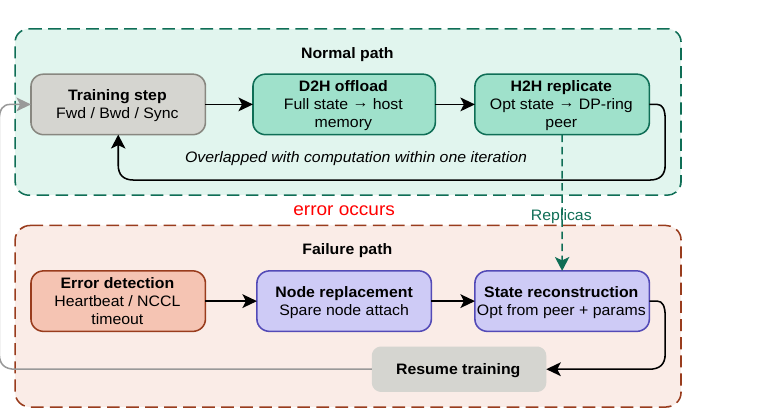
1. Asynchronous Offload Pipeline (normal path, green in Figure 2): runs once per training iteration, copying the full rank state to host memory and replicating the optimizer-state shard to a peer, both fully overlapped with forward/backward/gradient-sync computation.
2. Error Detection and Isolation (failure path trigger, orange in Figure 2): monitors heartbeats and NCCL timeouts, classifies the failure type, and traps the exception before it reaches (and kills) the job manager, holding surviving ranks at a barrier while a replacement is provisioned.
3. Recovery Policy (failure path body): attaches a spare node, rebuilds communication groups and shard placement, reconstructs the missing state (parameters from healthy peers, optimizer state from in-memory replicas), and resumes training from the last completed step.

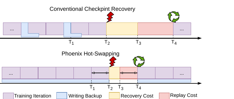
The paper visualizes the resulting timeline difference in Figure 3, comparing “conventional checkpoint recovery” against “PHOENIX hot-swapping”: in the conventional case, the periodic “writing backup” intervals sit on the critical path (small stalls interleaved with training), and after a failure at $T_2$, there is an explicit recovery-cost window ($T_2\!\to\!T_3$) followed by a much longer replay-cost window ($T_3\!\to\!T_4$) where previously-completed work is silently redone. In PHOENIX’s timeline, the backup work (blue, at the bottom of every iteration) is invisible — it happens underneath the training iterations rather than interrupting them — and after a failure, there is only a short recovery-cost window with essentially no replay window, because $T_3$ and $T_4$ nearly coincide.

The Asynchronous Offload Pipeline, step by step

The offload pipeline runs once per training iteration, overlapped with the same iteration’s forward pass, backward pass, and gradient synchronization. It has two phases with deliberately asymmetric payloads — this asymmetry is one of the more subtle, easy-to-miss design decisions in the paper, so it’s worth unpacking carefully.

Phase 1 — Device-to-host (D2H). The full rank state — optimizer-state shard, local model-parameter shard, and a small metadata envelope (step index, parallelism configuration, RNG states) — is packed into one contiguous buffer and copied asynchronously to pinned host memory, on a dedicated CUDA stream separate from the compute streams. Why copy the full state here, including parameters that are already redundant across DP peers? Because this D2H copy is purely local (GPU-to-host-memory over PCIe, no network involved), so it’s cheap, and having the complete state on the local host enables a fast local-only recovery path for transient GPU errors (Section VI-B’s error classification, below) without needing any network transfer at all — you don’t want to pay a network round-trip just to recover from a hiccup that didn’t actually lose any data.

Phase 2 — Host-to-host (H2H). Only the optimizer-state shard and the metadata envelope — not the model parameters — are sent over the network to a peer node in a ring topology (specifically, the DP-ring peer: same tensor-parallel and pipeline-parallel coordinate, different data-parallel index). A background worker thread waits for the D2H phase’s completion event, then sends the (smaller) optimizer payload via chunked MPI over the DP-local communicator.

Why exclude parameters from the H2H phase? This is the asymmetry, and the reasoning is a direct consequence of Insight 1 above: model parameters are already recoverable from a healthy DP peer at the same (TP, PP) coordinate via a collective communication at recovery time, so pre-replicating them to a peer in advance would consume network bandwidth without buying any reduction in recovery latency — you’d be protecting something that was never actually at risk of being unrecoverable. Local PCIe bandwidth (D2H) is generously available; inter-node network bandwidth (H2H) is the scarcer resource, so the design spends the scarce resource only on the state that has no other copy (the optimizer shard) and spends the cheap resource on everything (including a redundant copy of the parameters, purely for fast local transient-error recovery).

Here is the two-phase pipeline written out as pseudocode, matching the paper’s description:

Algorithm 1: Asynchronous Offload Pipeline (runs once per training iteration, per rank)
────────────────────────────────────────────────────────────────────────────
Input: rank state S = {optimizer_shard, param_shard, metadata}
        DP-ring peer node P
Output: recoverable replicas of optimizer_shard in local host memory and on P

 1: procedure OFFLOAD_ITERATION(S, P):
 2:     # --- runs concurrently with fwd/bwd/grad-sync on separate CUDA stream ---
 3:     buf_local ← pack(S.optimizer_shard, S.param_shard, S.metadata)  # contiguous buffer
 4:     async_copy(buf_local → pinned_host_memory, stream=D2H_stream)   # Phase 1: D2H
 5:     wait_for_event(D2H_stream.completion)                          # background worker waits
 6:     buf_peer ← pack(S.optimizer_shard, S.metadata)                  # smaller payload
 7:     async_send(buf_peer → P, comm=DP_local_communicator, chunked=True)  # Phase 2: H2H
 8:     # --- synchronization point ---
 9:     wait_before_optimizer_step()   # ensures peer-resident replica fully committed
10:     # optimizer.step() now safely mutates the protected state
11: end procedure

The single synchronization point that matters for correctness is on line 9: right before the optimizer mutates the protected state (i.e., right before optimizer.step()), the training loop waits for confirmation that the peer-resident replica is fully committed. In the common case — both D2H and H2H complete within the iteration’s compute window (forward+backward+grad-sync) — this wait observes an already-finished transfer and adds essentially zero exposed stall, which is exactly why the measured overhead is close to zero. The pipeline only becomes a bottleneck if the transfers are slower than the compute window, which the paper’s own communication-breakdown experiments (Figure 9, discussed later) show is not the case even in relatively communication-intensive small-scale configurations.

Ping-pong double buffering: why an in-progress copy never corrupts the recovery point

A natural worry with any “copy state to memory” scheme is: what if a failure happens during the copy itself? Is the in-memory replica now corrupted or partially written, and hence useless for recovery? PHOENIX solves this with a ping-pong double-buffering scheme, illustrated in Figure 5.

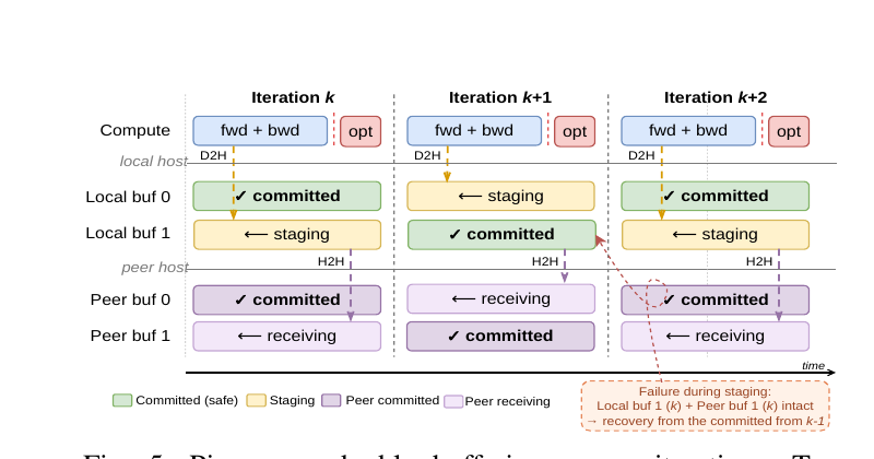
The scheme keeps two host-side buffers on the local machine (and, symmetrically, two buffers on the peer). At any given iteration $k$, one buffer holds the fully committed snapshot from the previous iteration $k-1$, while the other buffer is the staging target currently being written for iteration $k$. The roles swap every iteration: what was “staging” at iteration $k$ becomes “committed” at iteration $k+1$, and the buffer that was “committed” becomes the new staging target. The peer-side buffers follow the identical alternation pattern, just labeled “committed” and “receiving” instead of “committed” and “staging.”

Why does this guarantee correctness? Because only the currently-staging/receiving buffer can ever be left in a partially-written state by a mid-copy failure — the other buffer, holding the previous iteration’s fully-committed snapshot, is never touched during the current iteration’s copy and therefore remains completely intact and immediately usable. So even if a failure interrupts iteration $k$‘s D2H or H2H transfer, PHOENIX can always fall back to iteration $k-1$‘s committed snapshot — at worst, this costs one additional step of replay (the interrupted step $k$ itself), which is exactly the $t_\text{step}\cdot\mathbb{E}[\phi]$ term in Equation (5), never more. This is the mechanism that makes the “guarantee a valid recovery point is always present in host memory” property hold without requiring the offload itself to be atomic — you don’t need transactional writes when you simply never overwrite the only good copy you have.

Recovery Policy and the four correctness invariants

When a permanent failure is detected, PHOENIX needs a precise notion of what “correct” recovery means before it can claim its hot-swap procedure preserves training semantics. The paper states four invariants that must hold after recovery:

• I1 (Topology Consistency). All involved nodes agree on a single communication topology and shard placement — no two nodes can have different beliefs about who owns what.
• I2 (Shard Completeness). For every logical shard (of parameters or optimizer state), there exists exactly one valid owner among the involved nodes — no shard is duplicated (wasting resources / risking inconsistent updates) and none is missing.
• I3 (Optimizer Availability). The optimizer state for every shard is available from in-memory replicas — this is the invariant that the offload pipeline exists to guarantee.
• I4 (Step Atomicity). Training progresses in discrete steps; partial progress from a failed step is never committed — you either fully complete a step or you discard it and retry, never a half-applied update.

The recovery procedure, given these invariants as its acceptance criteria, executes in three ordered stages:

Algorithm 2: Recovery Policy (triggered on detected permanent node failure)
────────────────────────────────────────────────────────────────────────────
Input: failed_node F, pool of spare nodes SparePool, recovery descriptors
         of all surviving involved nodes
Output: training resumed from last completed step, invariants I1-I4 restored

 1: procedure RECOVER(F, SparePool):
 2:     # Stage 1: topology update
 3:     spare ← SparePool.acquire_one()
 4:     involved_nodes ← (involved_nodes \ {F}) ∪ {spare}
 5:     mark_topology_invalid()                       # pre-failure topology no longer usable
 6:
 7:     # Stage 2: quiesce + rebuild communication topology  → restores I1, I2
 8:     barrier_all(involved_nodes)                   # quiesce at a safe step boundary
 9:     new_topology ← rebuild_process_groups(involved_nodes)
10:     new_shard_map ← reassign_shard_ownership(involved_nodes, logical_shard_ids)
11:     assert single_owner_per_shard(new_shard_map)  # I2 check
12:
13:     # Stage 3: reconstruct missing state on the spare node → restores I3
14:     for shard in spare.assigned_shards:
15:         if shard.kind == PARAMETER:
16:             source ← find_healthy_peer(shard.logical_id, same_TP_PP_coordinate=True)
17:             spare.params[shard] ← targeted_collective_fetch(source, shard.logical_id)
18:         else:  # shard.kind == OPTIMIZER_STATE
19:             source ← find_in_memory_replica(shard.logical_id)  # from H2H replication
20:             spare.optimizer_state[shard] ← transport_fetch(source, shard.logical_id)
21:         end if
22:     end for
23:
24:     # Resume  → restores I4 (discard any partial progress from the interrupted step)
25:     discard_partial_step_state()
26:     resume_training_from(last_completed_step)
27: end procedure

A subtlety worth calling out explicitly: on line 16, model parameters are reconstructed via a targeted collective from a healthy node sharing the same logical partition (same TP/PP coordinate, different DP index) — this is the direct payoff of Insight 1 (parameters are naturally redundant, so they were never actively replicated, only reconstructed on demand at recovery time). On line 19, optimizer state comes from the in-memory replica that the H2H phase of the offload pipeline had been continuously maintaining — this is the payoff of the offload pipeline’s design choice to spend network bandwidth specifically protecting the one piece of state (optimizer shards) that has no natural redundancy elsewhere.

Another subtlety: source and replacement nodes are matched using logical shard identity derived from recovery descriptors, not post-failure rank indices. Why does this matter? Because after a node dies and a spare is attached, the numeric rank assignments in the distributed job can shift — the spare might not get the same rank number the failed node had. If shard-to-source mapping were done by rank index, a rank renumbering could silently pair the wrong source with the wrong destination. Matching by logical shard identity (essentially, a stable name for “the optimizer state belonging to layer X, DP-shard Y” that doesn’t change even if the physical rank number does) sidesteps this class of bug entirely.

Tolerating multiple simultaneous node failures

By default, PHOENIX replicates each optimizer-state shard to exactly one DP-ring neighbor (call this replication factor $k=1$), which tolerates any single node failure but not two nodes failing within the same step if both happen to hold copies of the same shard. To guard against this, PHOENIX supports configuring replication to $k$ distinct DP peers, at the cost of H2H network traffic scaling linearly in $k$ (still overlappable with computation for small $k$).

Quantifying shard-loss risk: independent vs. correlated failures

How risky is $k=1$ actually, in numbers? The paper works through this carefully, and the derivation is worth reproducing because it justifies a concrete engineering knob (whether to spend extra bandwidth on $k=2$) rather than leaving it as a hand-wave.

Independent-failure case. Assume replica placement is topology-unaware, so node failures are statistically independent. Using published statistics from a real 100K-GPU deployment (one interruption roughly every 18 minutes, step time roughly 20 seconds), the paper derives a per-node per-step failure probability of roughly $p \approx 10^{-6}$ (treated as a conservative upper bound). A specific shard is unrecoverable only if its owner and all $k$ replica holders fail within the same step, which under independence has probability $p^{k+1}$. Applying a union bound over $D$ data-parallel shards, the probability that any shard becomes unrecoverable in a given step is

$$P_\text{loss} \le D \cdot p^{k+1} \tag{6}$$

Plugging in $D=128$ and $k=1$: $P_\text{loss} \le 128 \times (10^{-6})^2 = 1.28\times10^{-10}$ per step, or cumulatively over a $10^5$-step run, $1.28\times10^{-5}$ — fewer than one unrecoverable-shard event per 100 full training runs. Bumping to $k=2$ pushes the cumulative probability down to $1.28\times10^{-11}$, which the paper reasonably calls “effectively zero.” Under the independent-failure assumption, then, $k=1$ is already extremely safe, and $k=2$ is overkill.

Correlated-failure case (the more realistic worry). The independence assumption breaks down when a shared infrastructure component — a top-of-rack switch, a network cable, a power distribution unit — fails and takes multiple co-located nodes down together. If a shard’s owner and its single replica happen to sit under the same switch, one switch failure destroys both copies simultaneously, which the pure per-node failure-rate math above completely misses. To address this, PHOENIX can use topology-aware placement: distribute the $k$ replicas across $k$ distinct failure domains (switches/racks), so a single infrastructure event can affect at most one copy of any given shard. Let $q$ denote the per-domain per-step failure probability (e.g., a ToR switch’s failure rate). With replicas spread across $k+1$ independent domains, the effective per-shard loss probability becomes $q^{k+1}$. Even at a relatively pessimistic domain failure rate $q=10^{-4}$: with $k=1$, cumulative risk over $10^5$ steps is $D\cdot q^2\times10^5 = 128\times10^{-8}\times10^5 = 0.128$ — non-negligible, roughly a 1-in-8 chance of some correlated shard loss somewhere in a full training run, which the paper flags as “non-negligible for safety-critical runs.” With $k=2$, this drops to $D\cdot q^3\times10^5 = 128\times10^{-12}\times10^5 = 1.28\times10^{-5}$, restoring the earlier “effectively negligible” regime.

The practical takeaway the paper draws: $k=1$ with topology-aware placement is adequate for the large majority of production scenarios (where correlated switch/rack failures are relatively rare events, not the dominant failure mode), while $k=2$ is worth the extra bandwidth specifically for environments experiencing frequent infrastructure-level (not just single-node) failures. This is a genuinely useful piece of quantitative guidance for anyone deploying a similar scheme — it turns “how many replicas should I keep” from a gut-feeling choice into a probability calculation you can actually run against your own cluster’s observed failure statistics.

Error Classification: not every failure gets the same treatment

A final piece of the design is recognizing that not all detected failures should trigger the (comparatively heavyweight, ~40s) node-replacement path. PHOENIX runs a classification layer that maps observed failure signals to one of several recovery actions:

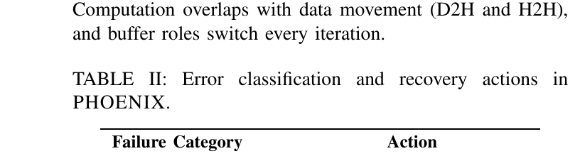
The logic: transient communication faults (the node is still up, its state is still valid, but a message got dropped or delayed) are handled with local recovery first — if the node remains responsive, there is no need to replace it at all, only to reset and reinitialize it as if it were a fresh replacement (the paper treats this uniformly as a degenerate case of “hot-swapping” where the failed node re-enters the system after a local reset). GPU memory faults, PCIe/host/kernel/reboot faults, and network/storage faults, by contrast, genuinely compromise the node’s ability to safely continue participating (device-level or system-level failures that prevent the node from reliably holding or computing its assigned shards), so these always trigger full node replacement. Software bugs, numerical errors, and silent data corruption are explicitly routed to an external fallback mechanism, entirely outside PHOENIX’s scope — the system makes no claim about handling failures where the training semantics themselves might be compromised, only failures where a node becomes unavailable or unreliable as a compute/storage resource.

This classification matters practically because it avoids the worst-of-both-worlds failure mode where every minor communication blip triggers an expensive full node-replacement procedure — without it, a system’s effective MTBF for triggering recovery could be much lower than its true rate of unrecoverable node loss, needlessly eating into training efficiency via Equation (4).

Design Choices: Why This Way, What Was the Alternative, Where Does It Break

Before moving to the experiments, it’s worth pausing on several non-obvious design decisions and asking why they were made this way, what the obvious alternative would have been, and where the chosen approach could fail.

Why in-memory replication instead of a faster persistent checkpoint? The obvious alternative to PHOENIX’s whole approach is simply making disk-based checkpointing faster — this is exactly what prior systems like CheckFreq, Gemini, and FastPersist do, via techniques like overlapping I/O with computation, hierarchical memory staging, and parallel NVMe writes. Why isn’t “just make disk checkpointing fast enough to do every step” sufficient? Because even an infinitely fast write doesn’t help if the failure itself destroys the ability to read it back quickly — the restart cost (re-initializing torch.distributed, filesystem I/O for the read-back, consistency verification) is largely independent of how fast the write was. In-memory replication to a peer sidesteps this because the replica lives on a different, still-healthy machine, reachable over the network without any filesystem round-trip, and recovery doesn’t require tearing down the whole distributed job to get to it. The boundary condition: this only works as long as the peer holding the replica is itself healthy. If both a shard’s owner and its replica peer die in the same step (Section on correlated failures above), you’re back to needing a persistent checkpoint as a fallback — the paper doesn’t discuss what happens in that (rare but nonzero) case beyond the topology-aware mitigation, which is a gap worth noting (see Limitations below).

Why asymmetric payloads (full state via D2H, optimizer-only via H2H) rather than symmetric replication of everything? As explained above, this follows directly from the observation that parameters are already redundant across DP peers while optimizer state is not. The alternative — replicate everything to the peer, symmetric with the local D2H copy — would be simpler to reason about but would roughly double the H2H network traffic for no correctness benefit, since the extra parameter copies would never actually be used (recovery always reconstructs parameters from a healthy DP peer via collective, never from the H2H replica). The boundary condition here is subtle: this asymmetry is a direct consequence of the specific redundancy structure of the 3D-parallel layout the paper studies. If a training framework’s parallelism scheme did not naturally replicate parameters across some redundant group (e.g., certain expert-parallel MoE layouts where each expert-holding node has no redundant peer), this asymmetric design would need to be revisited, because the “parameters are free to reconstruct” assumption would no longer hold.

Why ping-pong double buffering instead of a single buffer with atomic write semantics? The obvious alternative is to make the single-buffer write atomic (e.g., write-to-temp-then-rename, common in filesystem checkpointing) so a partial write never corrupts the one buffer you have. But atomic writes for large in-memory buffers being actively used by the training process are more awkward to implement correctly and can require extra copies or locking that adds latency to the critical path. Ping-pong buffering achieves the same guarantee (never having only a corrupted copy available) more cheaply, at the cost of doubling the host-memory footprint for the offloaded state. The boundary condition: this doubles host memory usage for the checkpoint buffers specifically, which is a real cost on memory-constrained host systems (though the paper’s target systems have hundreds of GB of host RAM, so this is unlikely to bind for models up to the 65B scale tested).

Why per-step protection instead of adaptive/less-frequent protection at larger scale? One might imagine that at very large scale, where D2H/H2H costs are a vanishing fraction of the (dominant) compute time (as Figure 9-left shows), per-step protection is clearly worth it — the marginal cost is nearly free. But at small scale or with communication-heavy topologies (Figure 9-right, the 2-node/8-GPU case), the per-rank offload payload is proportionally larger relative to the compute window, so per-step protection is a more demanding ask. The paper shows it still fits within the compute window in the tested configurations, but doesn’t fully characterize where the crossover point is — an adaptive scheme (protect every step when cheap, back off to every few steps when the offload payload threatens to exceed the compute window) is a natural extension the paper doesn’t explore.

Implementation

PHOENIX is implemented as a hybrid design: a data-plane extension integrated directly into Megatron-LM (reusing its distributed-optimizer serialization, sharded optimizer abstractions, and 3D-parallel process-group organization, so failure-free execution is unchanged when the mechanism is disabled — there is no redundant checkpoint stack bolted on the side), plus an external control plane implemented as a standalone TCPStore-based coordination service running as an independent process. Keeping the control plane out-of-process is deliberate: it remains available and able to coordinate recovery even when a subset of training processes have crashed, which wouldn’t be true if the coordination logic itself lived inside the training processes.

The implementation spans four components: (1) a program entry path for registering with the control plane and initializing failure-aware execution, (2) a training-step scheduler enforcing safe quiescence and recovery boundaries (the barrier logic in Algorithm 2), (3) a checkpoint/optimizer wrapper maintaining the in-memory recoverable state (the ping-pong buffers), and (4) an asynchronous MPI-based transport service handling both the H2H replication during normal operation and the state-restoration transfers during recovery.

A nice engineering property worth highlighting: because PHOENIX is an opt-in extension rather than a wrapper sitting outside the training loop, when the mechanism is disabled there is genuinely no interception layer left in the hot path — the failure-free execution path is unchanged, not just “fast because the overhead happens to be small.”

Experimental Evaluation

The evaluation targets two production HPC systems — Perlmutter at NERSC (HPE Cray EX, A100 GPUs, Slingshot 11 interconnect, dragonfly topology) and Vista at TACC (NVIDIA Grace-Hopper superchip nodes, H200 GPUs, NDR InfiniBand, fat-tree topology) — training GPT-style transformers from 0.6B to 65B parameters, on Megatron-LM with 3D parallelism and ZeRO-2, using full-precision (FP32) training throughout to maximize per-rank state volume (a deliberately demanding, worst-case setting for PHOENIX’s offload path, since FP32 optimizer state is the largest it can be). The evaluation asks two core questions: does per-iteration in-memory checkpointing add any measurable overhead as the system scales, and does hot-swap recovery stay efficient as scale grows?

Checkpoint overhead is statistically indistinguishable from zero

Figure 6 shows same-topology weak scaling for a 2.3B model with TP=4, PP=4 fixed, scaling from 32 to 256 GPUs while proportionally increasing the global batch size to keep per-rank workload constant.

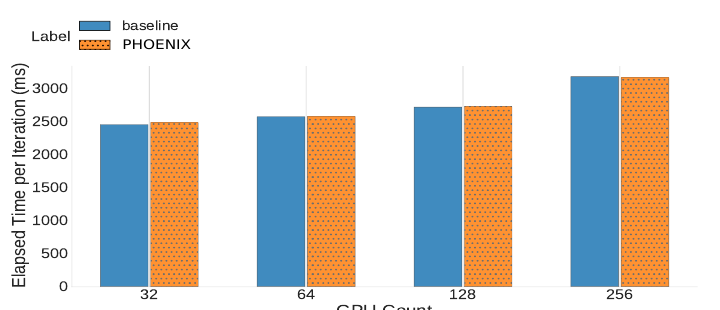
The numbers: at 8 nodes (32 GPUs), baseline averages 2442.13ms vs. PHOENIX’s 2470.15ms; at 16 nodes, 2560.35ms vs. 2561.75ms (nearly identical); at 32 and 64 nodes, PHOENIX is marginally faster than baseline (2696.62ms vs. 2701.87ms, and 3122.86ms vs. 3134.81ms respectively) — a reminder that these differences are within normal run-to-run measurement noise rather than a systematic effect in either direction. The methodology here is sound: the paper discards the first 10 iterations as warm-up and trims the slowest 5% of remaining iterations before averaging, standard practice for filtering out one-off stalls unrelated to the mechanism being measured. Crucially, there’s no trend of growing overhead as GPU count increases, which is the pattern you’d expect to see if the offload pipeline were becoming a bottleneck at scale — its absence is good evidence the overlap-with-compute design is actually working as intended, not just working by coincidence at the tested scales.

Figure 7 broadens this to six different 3D-parallel topology configurations (varying the DP/TP/PP split) across four model sizes (0.6B, 1.4B, 2.3B implied, plus larger), on 16 and 8 GPUs:

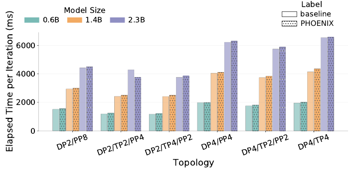
Across all six topologies, PHOENIX closely tracks baseline, with occasional small positive or negative deviations the paper attributes to normal run-to-run and node-allocation variability rather than a persistent overhead pattern. To check this generalizes across hardware, Figure 8 repeats the exercise on Vista’s Grace-Hopper nodes (H200 GPUs, InfiniBand) with 7B, 21B, and 65B models on 64 nodes:

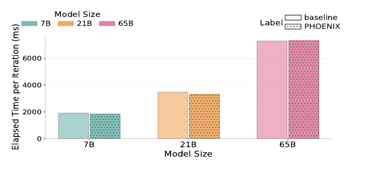
At 7B: 1854.5ms (PHOENIX) vs. 1912.8ms (baseline); at 21B: 3311.3ms vs. 3479.4ms; at 65B, effectively identical (7316.2ms vs. 7312.0ms). Interestingly PHOENIX is nominally faster in two of these three comparisons, again attributable to run-to-run noise rather than a genuine speedup — but the key point stands: the zero-overhead property holds across two entirely different GPU architectures (A100 vs. H200) and two different interconnect fabrics (Slingshot vs. InfiniBand), which is reasonably strong evidence this isn’t an artifact specific to one hardware generation.

Communication breakdown: why the overlap actually holds

Figure 9 decomposes per-iteration time into forward/backward compute (F/B), D2H, and H2H components, both for the same-topology weak-scaling setup (left) and for a more communication-intensive 2-node/8-GPU setting across three topologies (right):

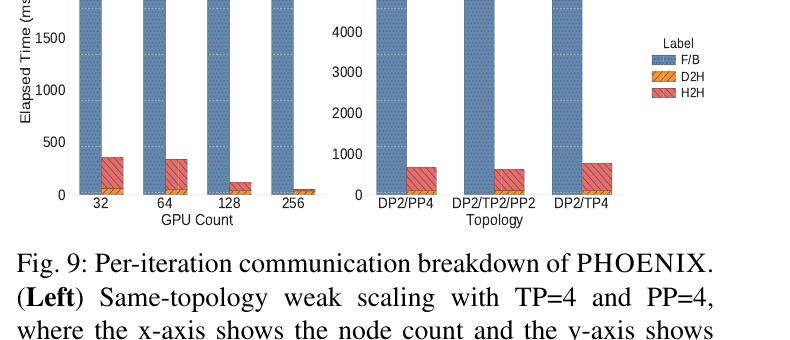
The left panel explains why PHOENIX’s overhead shrinks with scale: increasing the data-parallel degree reduces the amount of optimizer state each individual rank must offload (since ZeRO-style sharding spreads optimizer state more thinly across more ranks), so the offload path becomes a smaller and smaller fraction of the compute window as the system grows. The right panel stress-tests the opposite regime — a small 2-node cluster where each rank’s checkpoint payload is proportionally larger — and shows that even here, D2H+H2H costs remain comfortably below the compute window (5.6-6.4 seconds), leaving enough slack for the overlap to succeed. This is a good example of a paper actually probing the boundary condition of its own claim (“does this still hold when the payload-to-compute ratio is worse?”) rather than only reporting the friendliest configuration.

Recovery latency stays flat across model scales, grows slowly with cluster scale

Figure 10 fixes the cluster size at 128 GPUs and varies model size from 0.6B to 50B, plotting recovery-time breakdown (reconfiguration, parameter restoration, optimizer restoration) alongside measured GPU memory utilization:

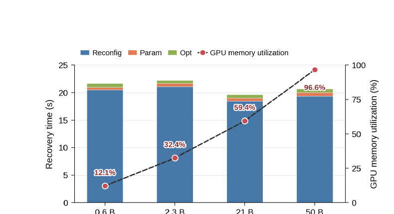
The headline result: recovery time is essentially independent of model size and memory pressure, even as GPU memory utilization rises nearly 8x (from 12.1% to 96.6%). The recovery-time bar is overwhelmingly dominated by the blue “Reconfig” (topology reconfiguration / NCCL rebuild) segment, with parameter restoration (orange) and optimizer-state restoration (green) contributing only thin slivers regardless of model size. This is a genuinely important finding: it means the actual state-transfer part of recovery (which one would naively expect to scale with model size, since bigger models mean bigger shards to restore) is not the bottleneck at all — the bottleneck is purely the mechanical cost of rebuilding communicator groups, which depends on cluster topology, not model size.

Figure 11 then fixes per-GPU memory utilization high and instead varies cluster size from 64 to 512 GPUs (weak-scaling the cluster):

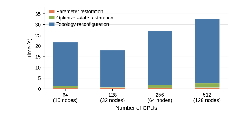
Recovery latency grows from 17.1s (32 GPUs) to 29.8s (512 GPUs) — growth that tracks the growth of topology-reconfiguration time (larger clusters mean more NCCL communicator state to rebuild), while parameter and optimizer restoration remain nearly flat across scales. Put together, Figures 10 and 11 support a clean, falsifiable claim: PHOENIX decouples recovery cost from model size, and its (mild) dependence on cluster size is attributable to a well-understood, specific cause (communicator reconstruction), not to anything about the state-restoration mechanism itself.

For context, checkpoint-restart in the same experimental setup averages 150 seconds for full distributed re-initialization, checkpoint loading, and process synchronization, versus PHOENIX’s under-40-second hot-swap — a >3.7x reduction in raw recovery latency, before even accounting for the additional replay-cost savings quantified next.

Real-world benefit quantification: the headline 18.8x number

The paper’s final experiment combines measured recovery costs with a Monte-Carlo-sampled failure process (using the failure rate from Meta’s 100K-GPU deployment study) to estimate real end-to-end impact. Setup: a 2.3B model training on 64 nodes for 100K steps, persistent checkpoints every 5K steps (8.9s per checkpoint write), 2.08s per step, total baseline runtime 2.41 days. Two sampled failure events land at 18 and 2366 steps after the most recent checkpoint respectively.

For these two failures, PHOENIX requires 32.6s and 29.8s respectively to resume to the original training progress. Checkpoint-restart, by contrast, requires 150s per recovery plus replaying all lost work since the last checkpoint — for the failure at step 2366-since-checkpoint, that’s 2366 steps of wasted recomputation at 2.08s/step, roughly 82 minutes, dwarfing the 150s restart cost itself (echoing the earlier analytical observation that replay, not restart mechanics, dominates checkpoint-restart’s cost at scale). Overall, PHOENIX reduces failure-induced recovery time to 5.3% of checkpoint-restart’s, an 18.8x reduction in time-to-resume. The paper notes (reasonably) that this advantage should grow, not shrink, as system scale increases and failures become more frequent, since PHOENIX avoids both repeated checkpoint loading and full-job restarts — both of whose relative cost only gets worse as $\text{MTTF}_\text{sys}$ shrinks (Equation (4)).

Limitations and Boundary Conditions

The paper is reasonably candid about some limitations, but several deserve more emphasis than they receive in the text:

• Only tested up to 512 GPUs and 65B parameters. Current frontier LLM training runs at 10,000-100,000+ GPU scale and models well beyond 65B parameters (the FT-HSDP citation itself references O(100K)-GPU deployments). The paper explicitly hedges with “we expect PHOENIX to be effective across many other GPU-dense supercomputers” and argues the checkpoint overhead is “one order of magnitude lower than computation” on current-generation hardware — but this is an extrapolation, not a measurement, and the topology-reconfiguration cost that dominates recovery latency (Figures 10, 11) is exactly the term that could scale unfavorably at 100K-GPU scale, since NCCL communicator rebuild cost is known to grow with participant count.
• Explicitly excludes silent data corruption and software bugs. These are real, non-negligible failure categories in practice (the paper’s own background section cites research quantifying how silent data corruption can alter trained model parameters) — PHOENIX’s entire correctness argument (the four invariants) assumes failures are cleanly detectable. A system that handles the “easy” 3 out of 4 failure categories well while punting the hardest one (silent corruption) to an unspecified “external fallback mechanism” is providing a real but partial solution, and readers should not conflate “tolerates all hardware faults” with “tolerates all faults.”
• Depends on generic capabilities that not every framework provides identically. PHOENIX’s design explicitly assumes sharded model/optimizer states, host-side spare-node management, shared recovery coordination, and runtime process-group reconstruction. The paper states these are “generic capabilities,” but runtime communicator reconstruction (rebuilding NCCL process groups without a full torch.distributed.init_process_group from scratch) is a genuinely non-trivial engineering capability that not all training stacks expose cleanly — the ease of porting PHOENIX to a framework other than Megatron-LM is asserted, not demonstrated.
• The Monte Carlo real-world benefit estimate uses only two sampled failure events. The 18.8x headline number is derived from a single Monte Carlo trajectory with exactly two failures, not an averaged distribution over many sampled trajectories with confidence intervals. This makes the number illustrative rather than statistically rigorous — a different random seed could plausibly produce a somewhat different multiplier, and the paper doesn’t report the variance.
• Spare-node provisioning is assumed available on demand. The recovery procedure assumes a spare node can be acquired immediately (line 3 of Algorithm 2). In a real production cluster under heavy contention, waiting for a spare node allocation could itself become a bottleneck the 40-second figure doesn’t account for — this is analogous to the “re-enter an already congested queue” problem the paper itself criticizes in checkpoint-restart’s restart path, and it’s not obvious PHOENIX is fully immune to the same issue if spare capacity isn’t pre-reserved.

Critical Analysis

Weaknesses and flaws specific to this paper. First, the evaluation scale gap is the most significant concrete weakness: the paper repeatedly frames its motivation around O(100K)-GPU deployments (citing FT-HSDP’s 18-minute MTBF and 10-minute restart stalls as the problem to solve) but evaluates only up to 512 GPUs — roughly 200x smaller than the scale that motivates the work. Since topology-reconfiguration cost (the dominant recovery-time component) plausibly scales with participant count in ways the paper’s own 32-to-512-GPU sweep (17.1s to 29.8s, less than 2x growth over a 16x scale increase) may not extrapolate linearly from. A log-log or explicit scaling-law fit of recovery time vs. cluster size, extrapolated to 100K GPUs, would have substantially strengthened the paper’s central motivating claim rather than leaving readers to take the extrapolation on faith. Second, the paper’s cost model (Equations 1-5) is elegant but rests on a uniform-failure and independent-failure approximation for the headline formulas, with the more realistic correlated/bursty failure treatment relegated to a secondary analysis (the topology-aware placement discussion) that isn’t integrated back into the main efficiency formula (Equation 4) — a reader can’t easily see how $\eta$ changes once correlated failures are accounted for. Third, the real-world benefit quantification (Section VII-C) uses a strikingly small sample (two failure events from one Monte Carlo trajectory) to produce a headline multiplier (18.8x) that gets prominently repeated in the abstract and conclusion; this is a case where the paper’s most citable number is also its least statistically robust one.

Limitations the authors understate or omit. The paper is notably quiet about control-plane fault tolerance — the TCPStore-based control plane is described as providing “a persistent coordination layer independent of the training processes,” but what happens if the control-plane process itself fails is left entirely to “future work” in the conclusion, with no discussion of how common such a failure might be or what its blast radius would look like (does control-plane failure mean the entire recovery mechanism is unavailable until it’s manually restarted?). Given that the whole point of the paper is eliminating single points of catastrophic failure in the training pipeline, a control plane that is itself a potential single point of failure for the recovery mechanism specifically deserves more than a one-line forward reference. Similarly, the paper doesn’t discuss what happens under truly pathological conditions like a cascading failure — a node failing during an active recovery epoch (the paper states “recovery epochs are serialized, so a new recovery begins only after the current one completes,” which implies a second failure during an in-progress recovery would simply have to wait, but doesn’t characterize how long that wait could stretch under a burst of failures, which is exactly the scenario where a large, degraded cluster is most likely to need robust recovery). Finally, the paper’s claim that disabling the mechanism yields “zero overhead” because “no interception layer is present in the training loop” is architecturally plausible but not independently verified with a dedicated ablation showing before/after code paths or profiler traces — readers are asked to trust the implementation claim rather than seeing it demonstrated the way the runtime-overhead claim is (with Figures 6-9).

Concrete, specific improvement suggestions. (1) Report recovery-time scaling with error bars or a fitted scaling law across at least 3-4 orders of magnitude of cluster size (even if only via simulation beyond the 512-GPU hardware limit), explicitly extrapolating to the 100K-GPU regime the paper uses to motivate the work, rather than leaving readers to extrapolate the 32-to-512-GPU trend themselves. (2) Re-run the Monte Carlo real-world benefit quantification (Section VII-C) over at least dozens to hundreds of sampled failure trajectories and report the distribution (mean, variance, or a confidence interval) of the recovery-time-reduction multiplier, rather than a single two-failure trajectory’s result. (3) Add an explicit fault-tolerance story for the control-plane process itself — even a simple design (e.g., a lightweight replicated control-plane state, or a documented manual-restart runbook with measured MTTR) would close the most conspicuous gap in an otherwise thorough failure-handling design. (4) Characterize behavior under concurrent or cascading failures more rigorously than “recovery epochs are serialized” — specifically, measure end-to-end degradation when failures arrive faster than the ~20-40s single-recovery window, since this is the regime where a 100K-GPU cluster with an 18-minute MTBF could plausibly find itself. (5) Provide a dedicated micro-benchmark isolating and directly measuring the “disabled mechanism” code path against a genuinely unmodified Megatron-LM baseline (not just the same codebase with the mechanism toggled off), to substantiate the “zero overhead when disabled” claim with the same rigor applied to the “zero overhead when enabled” claim.

A Worked Numerical Example: Tracing Through the Cost Model

To make Equations (1)-(5) concrete, let’s trace through a small hypothetical scenario end-to-end, using round numbers loosely inspired by the paper’s own FT-HSDP-scale citation.

Suppose a cluster has $\text{MTTF}_\text{sys} = 18$ minutes $= 1080$ seconds, step time $t_\text{step}=20$ seconds, and checkpoints under the traditional scheme are taken every $K=100$ steps.

Checkpoint-restart, step by step:

1. Expected replay steps: $\mathbb{E}[R] \approx (K-1)/2 = 49.5$ steps (Equation 1).
2. Replay time: $t_\text{step}\cdot\mathbb{E}[R] = 20 \times 49.5 = 990$ seconds $\approx 16.5$ minutes.
3. Restart latency: say $\mathbb{E}[T_\text{restart}] = 600$ seconds (10 minutes, matching the FT-HSDP citation).
4. Checkpoint overhead (amortized): say $C_\text{overhead}^\text{ckpt} = 5$ seconds (small compared to the other two terms; the paper’s own experiments measure PHOENIX’s overhead as $\approx$0, and even optimized checkpointing schemes like CheckFreq/Gemini/FastPersist keep this small — it’s the other two terms that dominate).
5. Total disruption per failure (Equation 2): $\mathbb{E}[C_\text{ckpt}] = 5 + 600 + 990 = 1595$ seconds $\approx 26.6$ minutes.
6. Effective training efficiency (Equation 4): $\eta \approx \dfrac{1080}{1080+1595} = \dfrac{1080}{2675} \approx 0.404$ — i.e., under this (deliberately pessimistic, illustrative) parameterization, the cluster would spend only about 40% of wall-clock time actually training, with the remaining 60% lost to failure recovery and replay.

PHOENIX, step by step, same cluster:

1. Checkpoint overhead: $C_\text{overhead}^\text{PHOENIX} \approx 0$ (measured, not assumed — Figures 6-9).
2. Hot-swap latency: say $\mathbb{E}[T_\text{hotswap}] = 30$ seconds (within the paper’s measured under-40s range at moderate cluster scale).
3. Replay: at most one partial step, say $\mathbb{E}[\phi] = 0.5$ (failure lands halfway through the interrupted step on average), so $t_\text{step}\cdot\mathbb{E}[\phi] = 20\times0.5 = 10$ seconds.
4. Total disruption per failure (Equation 5): $\mathbb{E}[C_\text{PHOENIX}] = 0 + 30 + 10 = 40$ seconds.
5. Effective training efficiency: $\eta \approx \dfrac{1080}{1080+40} = \dfrac{1080}{1120} \approx 0.964$ — roughly 96.4% of wall-clock time spent actually training.

The ratio of disruption costs here is $1595/40 \approx 40\times$, and the efficiency improves from roughly 40% to roughly 96% — a dramatic difference driven almost entirely by collapsing the replay term from 990 seconds down to 10 seconds (eliminating checkpoint-interval replay) and the restart term from 600 seconds down to 30 seconds (eliminating full-job restart). This toy calculation, while using illustrative rather than paper-reported numbers for some terms, demonstrates why the paper’s real Monte Carlo experiment (Section VII-C, with its 18.8x number) lands in a broadly similar ballpark — the mechanism driving the improvement is structural (both cost terms shrink by roughly an order of magnitude or more), not a fragile artifact of one specific parameter choice.

Frequently Asked Questions

Does PHOENIX replace persistent checkpointing entirely? Not necessarily in practice, though the paper’s design could in principle support it. The in-memory replicas protect against node failures during a training run, but they don’t survive a full cluster power-down or a need to resume training days later on entirely different hardware. Most real deployments would likely still want occasional persistent checkpoints (at a much coarser interval, since PHOENIX handles the common case) as a durability backstop for scenarios in-memory replication can’t cover — the paper doesn’t explicitly discuss whether/how it expects the two mechanisms to coexist, which is itself a minor gap.

What happens if a spare node isn’t immediately available? Algorithm 2 assumes SparePool.acquire_one() succeeds promptly. As discussed in the Limitations section, the paper doesn’t characterize behavior under spare-node contention, which could erode the ~40-second recovery guarantee in a heavily-utilized shared cluster.

Does this work with mixed-precision (BF16/FP16) training? The evaluation deliberately uses full FP32 training throughout specifically to stress-test the worst case for offload payload size (larger optimizer state to move per rank). The paper argues this makes the zero-overhead result more, not less, convincing — if the mechanism doesn’t introduce overhead even when there’s more state to move, it should have even more slack under BF16/FP16 training, where the offloaded payload would be considerably smaller. This is a reasonable inference, but it is an inference rather than a directly reported measurement with mixed precision enabled.

Is the $k$ (replication factor) choice a static, one-time setting? As described, yes — $k$ is a deployment-time configuration choice (per-shard replication count and, optionally, topology-aware domain placement), not something PHOENIX adapts dynamically based on observed failure rates during a run. An adaptive scheme that raises $k$ temporarily after observing a burst of failures is a natural but unexplored extension.

Reproducibility Notes

The paper is built on public, well-documented infrastructure — PyTorch and Megatron-LM — and the core algorithmic ideas (ping-pong double buffering, asymmetric D2H/H2H payloads, logical-shard-identity-based recovery matching) are described with enough procedural detail (Sections V-B through V-C, VI-A through VI-F) that a competent distributed-systems engineer could reimplement the core mechanism, even without released code. That said, several practical details needed for exact reproduction are not fully specified in the text: the precise heartbeat/timeout thresholds used for error detection, the exact spare-node pool sizing and provisioning latency assumptions, and the specific NCCL/communicator-rebuild implementation details that dominate recovery latency (Figures 10-11) are described at the level of “what happens” rather than “exactly how, with what parameters.” No public code repository is referenced in the version of the paper reviewed here; readers wanting to reproduce the exact numbers would need access to Perlmutter- or Vista-class hardware (or a comparable A100/H200 cluster with a fast interconnect) and would likely need to re-derive several implementation specifics from the paper’s prose description rather than from released source.

Conclusion

PHOENIX makes a genuinely compelling case that the long-assumed tradeoff between error-free overhead and recovery cost in fault-tolerant LLM training is not fundamental — it is a consequence of how prior systems chose to protect state (periodic, persistent, on-disk) and how they chose to recover (full job restart). By recognizing that 3D-parallel training already has built-in redundancy for model parameters (across DP peers) and by treating node failure as an online topology-repair problem rather than a full restart, PHOENIX achieves both zero measurable overhead during normal execution and consistent under-40-second hot-swap recovery, decoupled from model size and only mildly dependent on cluster size. The correctness argument (four invariants, ping-pong double buffering, logical-shard-identity matching) is carefully constructed and the experimental evaluation, while limited in absolute scale relative to the frontier-scale deployments that motivate the work, is methodologically sound within the scales it does test. The most important open question the paper leaves for future work — and one that matters more the larger training clusters get — is whether the topology-reconfiguration cost that already dominates recovery latency at 512 GPUs continues to be a small, bounded cost or becomes the new bottleneck at the 10,000-100,000-GPU scale where these failures actually happen most often in practice.