AdaFlash: Taming Variance in Diffusion Speculative Decoding

Review date: 2026-07-22 Review author: Zhongzhu Zhou Paper reviewed: AdaFlash: Adaptive Speculative Decoding via On-Policy Distilled Diffusion Drafters Paper authors: Yu-Yang Qian, Hao-Cong Wu, Chen Chen, Jiacheng Sun, Zhenhua Dong, Peng Zhao, Zhi-Hua Zhou arXiv: 2607.19223 Status: Preprint (Nanjing University / Huawei Noah’s Ark Lab collaboration), 2026-07-21

Short Answer

Speculative decoding speeds up LLM inference by letting a cheap “draft” model propose several tokens at once, which the expensive “target” model then checks in a single parallel pass. A recent trend replaces the usual autoregressive (token-by-token) draft model with a diffusion draft model that can propose an entire block of tokens in one forward pass — DFlash is the representative one-step diffusion drafter that this paper builds on. AdaFlash’s contribution starts from an empirical diagnosis: the very same bidirectional attention that lets a diffusion drafter see the whole draft block at once and finish in one pass also makes its draft quality wildly inconsistent — both across task domains (chat vs. code vs. math) and within a single draft sequence (early tokens vs. late tokens). A drafter tuned offline once and then frozen, verified against a fixed candidate length, cannot react to either kind of drift. AdaFlash proposes two complementary, always-on mechanisms that close this gap during live deployment: (1) an on-policy distillation (OPD) loop that continuously retrains the drafter using the target model’s own live feedback, with a reverse-KL objective and an entry-wise divergence-clipping trick tailored to the diffusion drafter’s tendency to spread probability mass too broadly; and (2) an adaptive length head, a tiny auxiliary network that predicts how many of the current draft’s tokens are likely to be accepted and truncates the verification request accordingly, so the expensive target model is never asked to check tokens that are almost certainly going to be rejected anyway. Measured end-to-end across eight benchmarks, three target models (dense and mixture-of-experts), and concurrency levels from 1 to 128 concurrent requests, AdaFlash consistently beats EAGLE-3, plain DFlash, and an existing online-distillation baseline (OSD), with the largest wins precisely where earlier diffusion-drafter methods degrade below plain autoregressive decoding: high-concurrency serving.

Key Takeaways

• The core diagnosis is variance, not accuracy. DFlash’s average draft quality is already good — the problem the paper identifies is that this average hides enormous swings: on Qwen3-8B the average accepted length $\tau$ ranges from 3.40 (ShareGPT chat) to 7.09 (MathQA), a 2.1× spread, versus only a 1.2× spread (3.89 to 4.60) for the autoregressive drafter EAGLE-3.
• Two distinct failure modes, two distinct fixes. Domain-level variance (drafter quality differs by task domain) is addressed by continuously retraining the drafter online (OPD). Token-level variance (drafter quality differs by position within one draft block, decaying toward the end) is addressed by dynamically shrinking the verification length per request (adaptive length head) rather than trying to fix the drafter itself.
• The distillation objective is reverse-KL, not the usual forward-KL/cross-entropy, because diffusion drafters trained with bidirectional attention tend to spread probability mass broadly (high entropy); reverse-KL is mode-seeking and concentrates the drafter’s mass onto the target model’s high-probability tokens, which is exactly what speculative decoding’s accept/reject rule rewards.
• A single design flaw in naive reverse-KL is patched with entry-wise divergence clipping: a handful of vocabulary entries where the drafter assigns noticeable probability but the target assigns almost none blow up the KL sum and can dominate (and destabilize) the gradient; clipping each term at a threshold $\delta$ before summing removes these outliers while keeping the informative signal from the rest.
• The length head is trained almost for free. Its supervision target — the fraction of draft tokens actually accepted — falls out of the speculative-decoding verification step that already has to run; no extra rollouts or auxiliary value network are needed, and its gradient is detached from the drafter so the two learning problems don’t interfere with each other.
• The systems engineering matters as much as the algorithm. An asynchronous training/inference split (so retraining never blocks token generation), lightweight hot-reloading of only the drafter’s parameters, and a variable-length-aware request scheduler with an EMA-based admission controller are all necessary to make “continuously retrain a model while it’s serving live traffic” practical rather than a research toy.
• The headline numbers: on Qwen3-8B at concurrency 1, AdaFlash reaches a 4.06× average speedup over standard autoregressive decoding versus 3.53× for plain DFlash, 3.95× for the OSD online-distillation baseline, and 2.34× for EAGLE-3. At concurrency 128 — where DFlash (0.76×) and OSD (0.83×) both fall below plain autoregressive decoding — AdaFlash still delivers a 1.15× speedup, and the paper reports gains of up to ~66% higher throughput than the next-best method in the highest-concurrency regimes.
• This is not free lunch without infrastructure: the paper is candid that on one of its three target models (Qwen3.5-9B, which uses a Gated DeltaNet architecture), the high-concurrency benefit shrinks because the serving engine (SGLang) doesn’t yet have an efficient implementation of variable-length verification for that specific architecture — a reminder that adaptive algorithms are only as good as the scheduler underneath them.

Prerequisites: What You Need to Know First

Autoregressive Decoding and Why It’s Slow

A standard (autoregressive, “AR”) large language model generates text one token at a time: to produce token $x_{i+1}$, it must have already produced $x_1, \dots, x_i$, feed the whole sequence back through the network, and sample from the resulting probability distribution over the vocabulary. This is inherently sequential — you cannot start computing token 5 before token 4 exists — and for a model with billions of parameters, every single one of those per-token forward passes is expensive. If generating a full response takes 500 tokens, you pay for 500 full forward passes through a huge network, even though modern GPUs are usually memory-bandwidth-bound during single-token decoding (the GPU spends most of its time moving weights, not doing floating-point work), which means a lot of that expensive compute capacity sits idle.

Speculative Decoding: The Basic Idea

Speculative decoding (Leviathan et al., 2023; Chen et al., 2023) exploits this idle compute by introducing a second, much smaller and faster “draft” model $q_w$. Instead of generating one token at a time with the big “target” model $p_v$, the pipeline works like this each round:

1. The draft model $q_w$ quickly proposes a sequence of $k$ candidate tokens (this is cheap because $q_w$ is small).
2. The target model $p_v$ runs a single forward pass over the whole candidate sequence — because transformer forward passes can score an entire sequence in parallel (this is what makes training fast too), checking $k$ tokens at once costs barely more than checking one, as long as the GPU had spare compute capacity.
3. For each candidate token $x_i$, it is accepted with probability $\min\{1, p_v(x_i \mid x_{<i}) / q_w(x_i \mid x_{<i})\}$ — i.e., accepted for sure if the target model liked it at least as much as the draft did, and accepted probabilistically otherwise.
4. All tokens up to the first rejected one are kept. At the rejection point, a corrected token is resampled from the residual distribution $\max(0, p_v - q_w)$ (renormalized), which is the mathematical trick that makes the whole procedure exactly lossless: the final output distribution is provably identical to what you’d get from running the target model alone, token by token.

The expected number of output tokens produced per round is

$$\mathbb{E}[\tau] = \frac{1-\mathrm{Acc}^{k+1}}{1-\mathrm{Acc}},$$

where $\mathrm{Acc} = \mathbb{E}_{x\sim q_w}[\min\{1, p_v(x\mid x_{<i})/q_w(x\mid x_{<i})\}]$ is the acceptance rate — the average probability that any given draft token survives. The overall wall-clock acceleration compared to plain AR decoding is

$$\eta = \frac{\mathbb{E}[\tau]}{\rho k + 1},$$

where $k$ is the candidate (draft) length and $\rho \ll 1$ is the ratio of the draft model’s per-round inference time to the target model’s. Two quantities control everything: how cheap the draft is ($\rho$) and how often its guesses are right ($\mathrm{Acc}$, which drives $\mathbb{E}[\tau]$). Everything in this paper is ultimately about improving one or both of those two quantities under realistic, shifting deployment conditions.

Diffusion Language Models as Drafters

A standard AR draft model still has to generate its $k$ candidate tokens one at a time — $k$ sequential forward passes through the (small) draft network. Diffusion language models (dLLMs) offer an alternative generation mechanism: instead of predicting the next token conditioned on everything before it, a dLLM is trained to take a sequence with some positions “masked” and predict all masked positions simultaneously, using bidirectional attention (each masked position can attend to both earlier and later context, including other currently-masked positions). Classic diffusion-style text generation runs this mask-and-predict step repeatedly, gradually “denoising” more and more positions — which still costs multiple forward passes and partially cancels the parallelism benefit.

DFlash (Chen et al., 2026), the direct predecessor this paper builds on, short-circuits that: given a prefix $x$, it initializes $k$ masked positions and generates the entire candidate block $\{x_1,\dots,x_k\}$ in a single forward pass through the bidirectional network:

$$\{x_1,\dots,x_k\} \sim q_w(\cdot \mid x, z),$$

where $z$ denotes the masked state of the draft block. Because the whole block comes from one pass rather than $k$ sequential ones, the time ratio becomes $\rho_{\text{dLLM}} \approx \rho_{\text{AR}}/k$ — the per-token drafting overhead is roughly $k$-fold smaller than an AR drafter’s, which lets DFlash afford a deeper, more expressive drafter network without paying extra latency, and empirically gives it both a cheaper draft step and a higher acceptance rate than comparable AR drafters.

Why Bidirectional Attention Is a Double-Edged Sword

This is the crux of AdaFlash’s contribution, so it’s worth spelling out carefully before the paper’s own notation takes over. An AR drafter’s prediction for position $i$ only ever depends on positions $1,\dots,i-1$ — the causal structure is identical at training time and at inference time, for every domain and every position, so its behavior tends to be fairly uniform. A diffusion drafter’s prediction for a masked position depends on the entire surrounding context, including other masked positions whose eventual values aren’t known yet. This gives it much richer contextual modeling — and lets it finish in one pass — but it also means the effective difficulty of predicting any given position depends heavily on exactly what surrounds it: how “in-distribution” the domain is, how deep into the block the position sits, how much the joint uncertainty over the other masked positions leaks into this one’s prediction. A drafter that was fine on math data can be badly miscalibrated on chat data; a drafter that nails the first few tokens of a block can fall apart by the last few. That’s the double edge: the mechanism that makes one-pass parallel drafting possible is the same mechanism that makes its quality unstable.

On-Policy Distillation: Learning From Your Own Mistakes, Live

Ordinary (“offline”) knowledge distillation trains a small student model to mimic a large teacher model’s outputs on some fixed training set, collected once before training starts. The problem in a deployment setting is distribution mismatch (also called exposure bias): the student is evaluated at test time on sequences it itself generated, which may look nothing like the offline training distribution — the student never saw its own generation mistakes during training. On-policy distillation (Agarwal et al., 2024) fixes this by having the student generate its own trajectory, then querying the teacher’s soft output distribution along that exact trajectory as the supervision signal. This is naturally suited to speculative decoding: the draft model already produces candidate sequences, the target model already computes its own distribution over those same positions during verification — so the “supervision” for on-policy distillation is a side effect of a step the pipeline was already going to do. Prior work (OSD, Liu et al., 2024) applied this idea with a standard forward-KL/cross-entropy loss; AdaFlash’s contribution here is adapting the objective itself (reverse-KL, not forward-KL) to suit a diffusion drafter’s specific failure mode, plus a stabilization trick (entry-wise clipping) that forward-KL distillation never needed.

Forward KL vs. Reverse KL: Why the Choice of Divergence Matters

Given a target distribution $p$ and a drafter distribution $q$ over a shared vocabulary, the two most common divergences used to pull $q$ toward $p$ are:

$$D_{\mathrm{KL}}(p \,\|\, q) = \sum_{y} p(y) \log \frac{p(y)}{q(y)} \qquad \text{(forward KL — "mode-covering")}$$ $$D_{\mathrm{KL}}(q \,\|\, p) = \sum_{y} q(y) \log \frac{q(y)}{p(y)} \qquad \text{(reverse KL — "mode-seeking")}$$

Forward KL is what ordinary cross-entropy training amounts to: it heavily penalizes $q$ for assigning low probability anywhere that $p$ assigns high probability, so the student is pushed to cover every mode of the teacher — even ones that are individually low-frequency but appear somewhere in the training data. This is the right choice when you want broad coverage (e.g., standard supervised fine-tuning). Reverse KL instead heavily penalizes $q$ for assigning probability where $p$ does not, so the student is pushed to concentrate its mass on whichever mode(s) of the teacher it finds easiest to represent, at the cost of not trying to cover the teacher’s full spread. For speculative decoding this asymmetry matters a lot: a draft token only needs to fall inside the target model’s high-probability region to be accepted with high probability — there is no benefit whatsoever to a drafter “covering” some obscure low-probability continuation the target model would rarely produce anyway. Diffusion drafters, precisely because bidirectional attention gives them a tendency toward high-entropy (broad, unfocused) output distributions, are especially prone to wasting probability mass on regions the target model doesn’t care about — which is exactly the failure mode reverse-KL is suited to correct.

Architecture Overview

The diagram below shows how AdaFlash’s two learned components — the diffusion drafter $q_w$ and the adaptive length head — sit around the frozen target model $p_v$ inside one speculative-decoding round, and how the online training loop feeds back into the drafter without blocking generation.

flowchart TB
    subgraph ServingLoop["Live Serving Round t"]
        A["Prefix x (context so far)"] --> B["Diffusion Drafter q_w:\nsingle forward pass,\nk masked positions"]
        B --> C["Candidate block\nx_1 ... x_k"]
        C --> D["Adaptive Length Head:\npredict acceptance rate a_hat_t"]
        D --> E["Truncate to k_hat_t = clamp(floor(a_hat_t * k), 1, k)"]
        E --> F["Target Model p_v:\none parallel forward pass\nover k_hat_t tokens"]
        F --> G["Accept/Reject rule:\nmin(1, p_v/q_w) per token"]
        G --> H["Accepted prefix + 1 resampled token\n=> output tokens for this round"]
    end
    subgraph TrainLoop["Asynchronous Training Worker"]
        F -.->|"target distributions\n(replay buffer)"| I["OPD Loss:\nmixture reverse-KL + hard-label CE\n+ entry-wise clipping"]
        G -.->|"ground-truth accept rate a*_t"| J["Length-Head Loss:\nMSE(a_hat_t, a*_t)"]
        I --> K["Updated drafter weights"]
        J --> L["Updated length-head weights"]
    end
    K -.->|"hot-reload\n(drafter + head only)"| B
    L -.->|"hot-reload"| D

Figure 1 (architecture): AdaFlash’s serving loop and training loop. The key structural point is that the target model $p_v$ is never touched by the training loop — only the drafter and the length head get hot-reloaded — so the expensive, frozen target model’s weights and KV cache management are completely undisturbed by continuous online learning.

Data-Flow / Pipeline Diagram: One Full Round, Step by Step

sequenceDiagram
    participant Client
    participant Drafter as Diffusion Drafter q_w
    participant Head as Length Head
    participant Target as Target Model p_v
    participant Trainer as Async Trainer

    Client->>Drafter: prefix x_<t
    Drafter->>Drafter: one forward pass, k masked positions
    Drafter->>Head: hidden state h_t (shared input)
    Head->>Head: linear + SiLU + mean-pool + sigmoid -> a_hat_t
    Head-->>Target: k_hat_t = clamp(floor(a_hat_t k), 1, k)
    Drafter->>Target: candidate tokens x_1..x_(k_hat_t)
    Target->>Target: single parallel forward pass
    Target-->>Client: accepted prefix + 1 resampled token
    Target-->>Trainer: p_v(.|x_<t+i) for i=1..k_hat_t (replay buffer)
    Target-->>Trainer: ground-truth accept fraction a*_t
    Trainer->>Trainer: compute OPD loss (reverse-KL + hard CE, clipped)
    Trainer->>Trainer: compute length-head MSE loss (detached)
    Trainer-->>Drafter: hot-reload updated weights (async, off critical path)
    Trainer-->>Head: hot-reload updated weights (async, off critical path)

Figure 2 (pipeline): Every arrow into the Trainer box is supervision that the pipeline was already producing as a byproduct of verification — nothing here requires an extra rollout, extra target-model call, or auxiliary reward model.

The Two Sources of Variance, Visualized

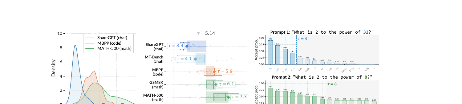
Panel (a) is the domain-level story: the acceptance-rate distribution for chat-style prompts (ShareGPT) is concentrated at low values with a sharp peak, while math-heavy prompts (MATH-500) concentrate at much higher values — these are not overlapping distributions, they are essentially different regimes. Panel (b) restates the same fact as accepted length $\tau$: MT-Bench/ShareGPT chat sits around $\tau \approx 3.3$–$4.1$, while GSM8K/MATH-500 math sits around $\tau \approx 5.9$–$7.3$ — very close to a 2× gap, all from the same, frozen drafter. Panel (c) is the token-level story within a single sequence: two prompts that differ by a single token (“2 to the power of 32?” vs “2 to the power of 8?”) produce accepted lengths of 4 and 8 tokens respectively — the per-position acceptance probability decays steadily as the draft block goes on, and how quickly it decays is itself unpredictable from the prompt alone. This is the empirical basis for building two separate fixes rather than one: the domain-level gap needs the drafter itself to move (retraining), while the token-level decay needs the system to react per-request (dynamic truncation) since no amount of retraining removes decay that is intrinsic to how far into a block a position sits.

Method Part 1: On-Policy Distillation (OPD) for Diffusion Drafters

Algorithm, Step by Step

The core idea is a continuously running “draft → feedback → adapt” loop, exploiting the fact that the target model’s verification step already computes exactly the supervision signal a distillation loss needs.

Algorithm 1: On-Policy Distillation Loop (per training round $t$)

1.  Given prefix x_<t, sample candidate block {x_1, ..., x_k} ~ q_w(. | x_<t, z)
    from the CURRENT diffusion drafter q_w (this is the same draft step
    the serving pipeline already performs).
2.  Send the candidate block to the target model p_v for verification
    (also already happening in the serving pipeline).
3.  Record, for every position i = 1..k, the target model's full output
    distribution p_v( . | x_<t+i ) -- this is available for free because
    verification already computes it, no extra target-model call needed.
4.  Compute the hard-label cross-entropy against the target's own top-1
    token x*_i = argmax_x p_v(x | x_<t+i):
        l_hard = -(1/k) * sum_i log q_w(x*_i | x_<t, z)
5.  Compute the reverse-KL divergence at each position i, but clip each
    individual vocabulary entry's contribution at threshold delta BEFORE
    summing over the vocabulary (Algorithm 2 below).
6.  Combine: l_OPD = alpha * l_hard + (1 - alpha) * l_rkl_clipped
7.  Backpropagate l_OPD through the drafter q_w only; accumulate into a
    replay buffer until 128 on-policy samples have been collected.
8.  Once the buffer is full, run AdamW for 2 epochs (effective batch
    size 2, max sequence length 2048), producing an updated q_w.
9.  Hot-reload only the updated drafter parameters into the live serving
    engine; the target model p_v is never touched.
10. Clear the buffer, go to step 1 with the newly updated drafter.

The crucial design property here is that every input to this loop — the candidate block, the target’s distribution, the ground-truth top-1 token — is something the serving pipeline computes anyway while doing ordinary speculative decoding. On-policy distillation adds a training step on top of an inference step that was already happening, rather than requiring a separate offline data-collection phase.

The Reverse-KL + Hard-Label Mixture Loss, Derived

Writing $[\,q_w(\cdot\mid x_{<t},z)\,]_i$ for the drafter’s distribution at position $i$ and $p_v(\cdot \mid x_{<t+i})$ for the target’s distribution at that same position, the two raw loss terms are

$$\ell_{\text{hard}} = -\frac{1}{k}\sum_{i=1}^{k} \log q_w(x_i^\star \mid x_{<t+i}), \qquad x_i^\star = \arg\max_x p_v(x \mid x_{<t+i}),$$ $$\ell_{\text{rkl}} = \frac{1}{k}\sum_{i=1}^{k} \mathrm{KL}\Big([q_w(\cdot\mid x_{<t},z)]_i \,\Big\|\, p_v(\cdot\mid x_{<t+i})\Big).$$

The intuition for combining them: $\ell_{\text{rkl}}$ alone gives a mode-seeking pull toward the target’s shape, but its gradient can be low-signal or noisy early in training, when the drafter’s distribution barely overlaps the target’s support at all (the log ratio can behave badly when $q_w(y)$ is non-negligible somewhere $p_v(y)$ is near zero). $\ell_{\text{hard}}$ is an ordinary cross-entropy against a single hard label — a much lower-variance gradient signal, but one that only tells the drafter about the single most-likely token, not the shape of the target’s whole distribution around it. Mixing the two with $\alpha \in [0,1]$,

$$\ell_{\text{OPD}} = \alpha\, \ell_{\text{hard}} + (1-\alpha)\, \ell_{\text{rkl}}^{\text{clip}},$$

gives the hard-label term a chance to anchor the drafter onto the correct top-1 token quickly and with low variance, while the (clipped) reverse-KL term continues sculpting the shape of the drafter’s distribution around that anchor. The paper’s own ablation (Table 3(a), reproduced below) sweeps $\alpha$ and finds monotonic improvement from $\alpha=0$ (pure reverse-KL) up to $\alpha=0.8$, then a slight regression at $\alpha=1.0$ (pure hard-label) — confirming that neither extreme is optimal and the mode-seeking regularization from reverse-KL remains useful even once hard-label supervision dominates.

Entry-Wise Divergence Clipping, Derived

Expanding the reverse-KL sum over the full vocabulary $V$ makes the failure mode concrete:

$$\mathrm{KL}(q \| p) = \sum_{y \in V} q(y) \log\frac{q(y)}{p(y)}.$$

Because diffusion drafters tend to produce high-entropy (broad) distributions, there will typically be a handful of vocabulary entries $y$ where $q(y)$ is non-negligible but $p(y)$ is extremely small — for these entries, $\log(q(y)/p(y))$ is large, and multiplying by even a modest $q(y)$ can make that single term dominate the entire sum, producing a gradient that is essentially responding to one outlier token rather than the overall shape mismatch (the paper visualizes this directly in its Figure 3, a token-by-token divergence heatmap of a GSM8K response, showing a small number of positions with divergence orders of magnitude above the rest). The fix is to cap each individual $(i, y)$ term at a threshold $\delta$ before summing:

Algorithm 2: Entry-Wise Clipped Reverse-KL

Input: drafter distribution q_w(.|x_<t,z) at each position i=1..k,
       target distribution p_v(.|x_<t+i) at each position,
       clipping threshold delta > 0
For each position i = 1 .. k:
    For each vocabulary entry y in V:
        term(i, y) = q_w(y | x_<t, z)_i * log( q_w(y|x_<t,z)_i / p_v(y|x_<t+i) )
        clipped_term(i, y) = min( term(i, y), delta )
    position_loss(i) = sum_y clipped_term(i, y)
l_rkl_clipped = (1/k) * sum_i position_loss(i)
return l_rkl_clipped

In closed form,

$$\ell_{\text{rkl}}^{\text{clip}} = \frac{1}{k}\sum_{i=1}^{k}\sum_{y\in V} \min\!\Big( [q_w(y\mid x_{<t},z)]_i \,\log\frac{[q_w(y\mid x_{<t},z)]_i}{p_v(y\mid x_{<t+i})},\ \delta \Big).$$

Why this design and not an obvious alternative? A more standard fix for outlier gradients would be plain gradient clipping (cap the norm of the whole gradient after backprop) — but that throws away information indiscriminately across all positions and vocabulary entries once the norm is over budget, including the informative ones. Entry-wise clipping instead targets the diagnosis directly: it identifies which specific (position, vocabulary-entry) pairs are responsible for the instability and caps only those, leaving the gradient signal from every other, well-behaved entry completely untouched. The paper’s own hyperparameter sweep (Table 3(b)) shows this trade-off precisely: no clipping gives a slightly-worse baseline; moderate clipping ($\delta=0.01$) gives the best accepted length and speedup; but overly aggressive clipping ($\delta \le 0.005$) starts to suppress useful gradient too, since at some point the threshold clips even ordinary, non-outlier divergence terms, which the paper reports slows convergence and reduces both accepted length and tokens-per-second. This is a textbook design-boundary: the mechanism helps because it’s targeted, but too aggressive a version of the same mechanism becomes indistinguishable from just deleting signal.

Method Part 2: The Adaptive Length Head

Motivation and Design

Even with a perfectly on-distribution drafter, positions later in a draft block are intrinsically harder to predict correctly than earlier ones — later positions depend on more of the (also-uncertain) surrounding masked context, so acceptance probability naturally decays along the block (Figure 3(c) above). If the system always verifies the full fixed candidate length $k$ regardless, it wastes the target model’s compute checking tokens that were unlikely to be accepted anyway — and worse, this waste compounds under high concurrency, where every wasted token of target-model compute is GPU time stolen from some other request that could have made real progress.

The adaptive length head is a small auxiliary network, attached to the same hidden state the diffusion drafter already computes, whose only job is to predict how much of the current draft is worth sending to the target model.

Algorithm 3: Adaptive Length Head, Forward Pass

Input: hidden state h_t in R^{k x H} (same input the drafter used),
       scale factor gamma (tunable, load-adaptive), block size k
1.  For each position i = 1..k:
        h'_i = SiLU( Linear(h_t[i]) )      # per-position projection, H' < H
2.  h_bar_t = (1/k) * sum_i h'_i            # mean-pool -> one global vector
3.  a_hat_t = sigmoid( Linear(h_bar_t) )    # scalar predicted accept rate
4.  a_hat_t = a_hat_t * gamma                # optional load-based rescaling
5.  k_hat_t = clamp( floor(a_hat_t * k), 1, k )
return k_hat_t                              # verification length for this round

Only the first $\hat k_t$ tokens of the draft are actually sent to the target model for verification — the rest are simply never checked, so the target model’s forward pass over this request is that much shorter (and, crucially, its cost scales with the actual per-request length rather than the worst-case fixed $k$).

Online Update of the Length Head, Derived

After the target model verifies the $\hat k_t$ tokens that were actually sent, the true acceptance fraction $a_t^\star \in [0,1]$ (the fraction of those tokens that were actually accepted) is immediately available — again, a free byproduct of a step the pipeline already performs. The head is trained with plain mean-squared error:

$$\ell_{\text{len}} = \big(\hat a_t - a_t^\star\big)^2.$$

An important, easy-to-miss design choice: the gradient of $\ell_{\text{len}}$ is explicitly detached from the drafter — it updates only the length head’s own parameters, never flowing back into $q_w$. Why does this matter? Because the drafter is simultaneously being updated by the (very different) OPD objective above. If the length-head’s MSE gradient were allowed to also flow into the drafter, the drafter’s parameters would be receiving two objectives pulling it in unrelated directions (match the target’s token distribution vs. make its own acceptance rate easier to predict), which could easily destabilize training or bias the drafter toward being “predictable” rather than “accurate.” Detaching keeps the two learning problems fully decoupled — the length head learns to track whatever the drafter’s current quality happens to be, without being able to influence that quality itself.

Why not just use a fixed candidate length tuned offline? The paper’s own ablation (Table 2, discussed below) answers this directly: with a fixed verification length set to the empirical average (11 tokens, matching AdaFlash’s own average of 11.271), speedup at concurrency 128 collapses to 1.00× — completely erasing the benefit of speculative decoding at high load, because at high concurrency the requests that would have accepted only 3–4 tokens are still forced to pay for verifying all 11. A fixed length picked to be reasonable on average is, by construction, wrong for every request that isn’t near the average.

Why per-position confidence instead of per-request confidence (comparison with DSpark)? A concurrent line of work, DSpark, tackles a similar problem by estimating a per-position conditional acceptance probability and applying a hardware-aware scheduler, but this requires post-hoc calibration to correct for compounding errors across positions (position 5’s probability estimate implicitly assumes positions 1–4 were accepted, and errors compound down the chain). AdaFlash’s design deliberately predicts the overall acceptance rate for the whole block directly from a single pooled representation, bypassing the need for that per-position probability calibration chain altogether — a simpler estimation target at the cost of not resolving which position within the truncated prefix is weakest (a boundary condition worth flagging, addressed in Critical Assessment below). The paper notes the two approaches are complementary rather than exclusive: DSpark’s hardware-aware scheduling could in principle be layered on top of AdaFlash’s length prediction.

Baseline / Prior-Art Comparison

Before looking at AdaFlash’s own numbers, it’s worth laying out exactly what each baseline in the paper’s comparison table represents, since “speculative decoding method” covers a fairly wide design space:

flowchart LR
    AR["Standard AR Decoding\n(no speculation, baseline 1x)"]
    EAGLE3["EAGLE-3\nAR feature-level drafter,\ntree-structured verification,\noffline trained, static"]
    DFlash["DFlash\ndiffusion drafter,\none-step block generation,\noffline trained, static, fixed k"]
    OSD["OSD\nDFlash drafter +\nonline forward-KL distillation,\nstill fixed k"]
    AdaFlash["AdaFlash (this paper)\nDFlash drafter +\nonline reverse-KL OPD\n+ adaptive length head"]
    AR --> EAGLE3
    AR --> DFlash
    DFlash --> OSD
    OSD --> AdaFlash
    DFlash --> AdaFlash
    style AdaFlash fill:#f9e0e0,stroke:#c0392b

Figure 4 (baseline taxonomy): the comparison set forms a clean ladder: EAGLE-3 represents the mature, offline-only AR-drafter school; DFlash is the offline diffusion-drafter baseline this paper’s method modifies; OSD adds some form of online adaptation but with the “wrong” divergence and no length adaptivity; AdaFlash is DFlash plus both of this paper’s contributions simultaneously. This ladder structure is exactly what supports the paper’s ablation methodology later (Table 2) — each step up the ladder isolates one added mechanism.

Experiments: What the Numbers Actually Show

Main Results (Table 1, reproduced)

Averaged across six benchmarks (MathQA, GSM8K, OpenCodeInstruct, CodeAlpaca, ShareGPT, Blend) with Qwen3-8B as the target model:

Method	Conc.=1 Speedup	Conc.=1 τ	Conc.=32 Speedup	Conc.=64 Speedup	Conc.=128 Speedup
EAGLE-3	2.34×	4.40	0.68×	0.43×	0.33×
DFlash	3.53×	5.86	1.54×	1.01×	0.76×
OSD	3.95×	7.05	1.70×	1.12×	0.83×
AdaFlash	4.06×	7.28	1.74×	1.33×	1.15×

Three things stand out. First, at concurrency 1 every method except EAGLE-3 is comfortably above 1× — the interesting regime is high concurrency. Second, every other method’s speedup crosses below 1.0× (i.e., becomes slower than plain AR decoding) by concurrency 128, while AdaFlash alone stays above 1×. Third, the gap between OSD and AdaFlash at concurrency 1 (3.95× vs. 4.06×, both using online distillation) is modest, but it widens sharply at concurrency 128 (0.83× vs. 1.15×) — this is the paper’s central empirical claim: online distillation alone (OSD) fixes domain-level variance but does nothing for the wasted-verification-cost problem that dominates at high concurrency, which only the adaptive length head addresses.

Ablation Study (Table 2, reproduced)

Divergence Clipping	Mixture OPD Loss	Length Head	Online Update	Conc.=1 τ	Conc.=1 Speedup	Conc.=128 τ	Conc.=128 Speedup
–	–	✓	✓	7.389	4.17×	6.802	1.18×
✓	–	✓	✓	7.590	4.31×	7.212	1.25×
✓	✓	✓	✓	7.751	4.54×	7.270	1.27×
✓	✓	–	–	–	–	6.594	1.00×
✓	✓	✓	–	–	–	7.652	1.21×
✓	✓	✓	✓	–	–	7.270	1.27×

Reading down the top block: adding divergence clipping on top of plain reverse-KL improves both accepted length and speedup at every concurrency; adding the hard-label mixture term on top of that improves further still — each OPD sub-component contributes independently, in the direction the design argument predicted. Reading the bottom block: removing the length head entirely (replacing it with the fixed average length 11) drops concurrency-128 speedup all the way to 1.00× — a complete loss of speculative decoding’s benefit at high load, matching the earlier main-table observation almost exactly. Adding the length head back with fixed (non-updating) parameters recovers most of the benefit (1.21×), and allowing it to keep updating online closes the rest of the gap (1.27×) — confirming that continual co-adaptation between drafter and length head, not just having a length head, is what sustains the benefit as the drafter’s own distribution keeps shifting under OPD.

Reproduced Effectiveness Figure

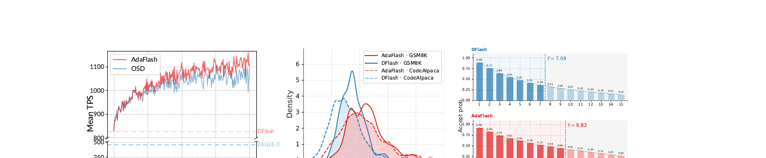
Panel (a) is a useful sanity check that online learning is actually converging rather than oscillating: mean tokens-per-second rises roughly monotonically (with expected noise) across 200 rounds and stabilizes above both the EAGLE-3 and DFlash reference lines. Panel (b) is the clearest single piece of evidence for the domain-level variance claim: DFlash’s acceptance-rate density for GSM8K and CodeAlpaca barely overlap (two separate humps), while AdaFlash’s densities for the same two datasets shift right and substantially overlap — direct visual confirmation that on-policy distillation is closing the domain gap, not just raising the average. Panel (c) shows the token-level story: DFlash’s per-position acceptance probability decays from about 0.89 at position 1 to about 0.13 by position 15, while AdaFlash’s decays more gently (0.92 to 0.26) — the drafter got better at every position, but proportionally more so at later ones, which is exactly why mean accepted length grows from 7.09 to 9.83.

Cross-Domain Generalization, NPU Portability, and Robustness Checks

The paper runs several supporting experiments worth noting briefly: (i) an AdaFlash drafter trained offline on a mixed “PerfectBlend” dataset (distinct from every individual test domain) and then evaluated without further online updates still beats offline DFlash across MathQA/GSM8K/OpenCodeInstruct/CodeAlpaca, though it lags behind the in-domain online-adapted version — evidence that some of OPD’s benefit transfers even without live per-domain adaptation, but the full benefit does require it; (ii) the same relative ordering (AdaFlash > DFlash) holds when the serving backend is swapped from GPU to a Huawei Ascend 910C NPU via SGLang-NPU, suggesting the method isn’t tied to one hardware stack; (iii) under stochastic sampling ($T=1$, rather than greedy $T=0$) accepted length drops for both DFlash and AdaFlash (expected, since a more diffuse target distribution makes exact token agreement less likely by construction), but AdaFlash retains a healthy 3.56× average speedup at concurrency 1; (iv) training an AdaFlash drafter completely from scratch (no pre-existing DFlash checkpoint) on a small target model (Qwen3-1.7B) still reaches 1.84× speedup versus 1.34× for EAGLE-3 under the same draft budget, showing the framework isn’t limited to fine-tuning an existing diffusion drafter.

Infrastructure: Making Online Adaptation Actually Deployable

An algorithm that continuously retrains itself during live serving is only useful if it doesn’t stall the very serving loop it’s trying to speed up. AdaFlash’s infrastructure section (built on SGLang) addresses two concrete requirements.

Asynchronous training/inference split. The system runs two logically separate workers connected by a shared replay buffer: an inference worker that serves live traffic and records on-policy trajectories (prompts + drafter responses + target distributions) into the buffer, and a training worker that asynchronously consumes the buffer, computes the OPD and length-head losses, and updates weights — entirely on separate GPU resources, so training compute never competes with, or blocks, token generation. Once new weights are ready, only the drafter and length-head parameters are hot-reloaded into the inference server’s GPU memory; the (much larger) target model’s weights and KV-cache state are never touched, so the reload itself completes between ordinary scheduling steps with negligible added latency.

Adaptive request scheduling for variable verification lengths. A standard serving engine (SGLang included) is built around fixed-shape batches: every request in a verification batch shares the same candidate length $k$. Once the adaptive length head makes $\hat k_t$ vary per-request, this assumption breaks, so AdaFlash modifies the engine to pack requests into a single verification batch whose total length equals $\sum_i \hat k_i$ rather than $N \times k$ — directly translating the length head’s per-request savings into a smaller, denser batch rather than padding everything back out to the worst case. Because the number of requests that fit into a fixed compute/memory budget now varies round to round (a batch of many short requests looks very different from a batch of few long ones), the scheduler tracks an exponential moving average of recently-observed request counts, $\hat N \leftarrow (1-\beta)\hat N + \beta N$, and uses $\hat N$ to decide how many new requests to admit into the next round; if actual memory usage still overshoots the budget, excess requests are returned to the pending queue rather than causing an out-of-memory failure. This is a fairly standard admission-control pattern (EMA-smoothed load estimate, graceful backpressure), but it is a necessary complement to the length head — without it, variable-length verification batches would either under-utilize the GPU (conservative fixed admission) or risk OOM (naive full admission).

A Fully Worked Numeric Example: Computing the OPD Loss for One Toy Position

To make the abstract formulas concrete, consider a single draft position $i$ with a toy vocabulary of just four tokens $\{A, B, C, D\}$. Suppose the drafter’s distribution and the target model’s distribution at this position are:

Token	$q_w(y)$ (drafter)	$p_v(y)$ (target)
A	0.55	0.80
B	0.30	0.15
C	0.10	0.04
D	0.05	0.01

Step 1 — hard-label term. The target’s top-1 token is $A$ (probability 0.80), so

$$\ell_{\text{hard}} = -\log q_w(A) = -\log(0.55) \approx 0.598.$$

Step 2 — raw reverse-KL terms per entry, $q_w(y)\log(q_w(y)/p_v(y))$:

• $A$: $0.55 \times \log(0.55/0.80) = 0.55 \times (-0.374) \approx -0.206$
• $B$: $0.30 \times \log(0.30/0.15) = 0.30 \times 0.693 \approx 0.208$
• $C$: $0.10 \times \log(0.10/0.04) = 0.10 \times 0.916 \approx 0.092$
• $D$: $0.05 \times \log(0.05/0.01) = 0.05 \times 1.609 \approx 0.080$

Summing: $\ell_{\text{rkl}} = -0.206 + 0.208 + 0.092 + 0.080 = 0.174$. Note that no single entry here is a wild outlier (all terms are within roughly a factor of 4 of each other), so with a clipping threshold $\delta=0.01$ used in the paper’s default configuration, every one of these four terms would actually get clipped down to at most 0.01 if this toy example’s terms were representative of a real, much-larger-vocabulary position — which is precisely the point: in a 100k+ token vocabulary, most of the probability mass sits on a handful of tokens like this toy example, but a small number of rare tokens can produce terms orders of magnitude larger (e.g., $q_w(y)=0.02$ against $p_v(y)=10^{-6}$ gives a term of $0.02 \times \log(20000) \approx 0.198$ from a single rare token alone) — clipping caps exactly those outliers while leaving well-behaved terms like the ones above essentially untouched if they’re already below $\delta$.

Step 3 — combine with $\alpha=0.8$ (the paper’s default):

$$\ell_{\text{OPD}} = 0.8 \times 0.598 + 0.2 \times 0.174 = 0.4784 + 0.0348 = 0.5132.$$

This single number is what gets backpropagated through the drafter for this one position; in practice it’s averaged over all $k=16$ positions in the block before the optimizer step.

Boundary-Condition Decision Diagram

The following captures, as a simple decision structure, when AdaFlash’s mechanisms are expected to help most versus when the paper’s own results suggest caution:

flowchart TD
    Start["Deploying a diffusion-drafter\nspeculative decoding system?"]
    Start --> Q1{"Decoding regime?"}
    Q1 -->|"Greedy (T=0)"| Q2{"Expected concurrency?"}
    Q1 -->|"Sampling (T>0)"| Caution1["Benefit still positive but\nless thoroughly validated\n(only 4/8 benchmarks, 2/4 concurrencies tested)"]
    Q2 -->|"Low (C=1)"| Good1["All methods including plain DFlash\nalready beat AR decoding;\nAdaFlash's edge is modest"]
    Q2 -->|"High (C>=64)"| Good2["This is AdaFlash's strongest regime:\nfixed-length methods fall below 1x,\nAdaFlash alone stays above 1x"]
    Good2 --> Q3{"Target architecture?"}
    Q3 -->|"Standard dense / MoE transformer"| BestCase["Full benefit demonstrated\n(Qwen3-8B, Qwen3-Coder-30B-A3B)"]
    Q3 -->|"Gated DeltaNet\n(e.g. Qwen3.5-9B)"| Caution2["Benefit narrows at C>=32:\nserving-engine variable-length\nscheduling not yet mature\nfor this architecture"]

Figure 6 (decision boundary): the paper’s evidence supports the strongest claims specifically in the greedy-decoding, high-concurrency, standard-transformer-architecture corner of this decision space; every branch away from that corner is still positive in the paper’s own numbers, but backed by thinner evidence.

Notation Reference

Symbol	Meaning
$p_v$	Target (large) model’s distribution
$q_w$	Draft (small, diffusion) model’s distribution
$k$	Draft block size (candidate length), fixed at 16 in experiments
$\hat k_t$	Adaptively truncated verification length at round $t$
$\mathrm{Acc}$	Acceptance rate (expected per-token accept probability)
$\tau$	Average accepted length per speculative round
$\rho$	Ratio of draft model inference time to target model inference time
$\eta$	Overall wall-clock acceleration factor
$\alpha$	Mixing coefficient between hard-label CE and reverse-KL in OPD loss
$\delta$	Entry-wise divergence clipping threshold
$\hat a_t$	Length head’s predicted acceptance rate for round $t$
$a_t^\star$	Ground-truth realized acceptance rate for round $t$
$\gamma$	Load-adaptive scale factor applied to $\hat a_t$
$\beta$	EMA smoothing coefficient for the request-count scheduler

Frequently Asked Questions

Does AdaFlash require retraining the target model? No — the target model $p_v$ is never modified; only the (much smaller) drafter and length head are updated online.

Does the online training add latency to any single request? Not directly — training runs on a separate GPU pool asynchronously; the only latency-relevant step on the serving path is the periodic hot-reload of updated drafter/length-head weights, which the paper describes as completing between scheduling steps.

Is AdaFlash specific to DFlash, or could it apply to other diffusion drafters? The paper builds directly on DFlash’s one-step block-generation mechanism, and the on-policy distillation/length-head design assumes that mechanism (a single forward pass producing a fixed-size candidate block); adapting to a multi-step diffusion drafter would likely require rethinking what “the hidden state the length head reads from” even means, since there would be several denoising passes rather than one.

What happens if the replay buffer never fills up (very low traffic)? The paper doesn’t explicitly address this; by construction, training is only triggered once 128 on-policy samples accumulate, so extremely low-traffic deployments would adapt very slowly, and the system would behave close to the static DFlash/OSD baselines until enough traffic accumulates.

Limitations and Boundary Conditions the Paper Acknowledges

• Greedy decoding is the default and the best-validated regime. Nearly every headline number in the paper (Table 1, Figure 2, the ablations) is measured under greedy decoding ($T=0$). The sampling-mode ($T=1$) results (Table 9) are reported only for four benchmarks at two concurrency levels, a much smaller slice of the experimental grid, and accepted length is noticeably lower across the board (e.g., $\tau \approx 6.42$–6.43 average vs. $\approx 8.20$ under greedy) — the paper is candid that sampling narrows the benefit but does not fully characterize how it scales at high concurrency the way the greedy results do.
• The Gated DeltaNet architecture exposes a real engineering gap. On Qwen3.5-9B, AdaFlash’s ShareGPT-domain speedup narrows or slightly reverses at concurrency $\ge 32$, and the paper attributes this explicitly to SGLang’s current lack of a fully efficient variable-length verification implementation for that specific architecture — a reminder that the adaptive length head’s benefit is bounded by how well the underlying serving engine can actually exploit variable batch shapes for a given model architecture.
• The block size $k=16$ is fixed across all experiments. The paper does not explore whether the diagnosis (domain/token variance) or the fix (OPD + length head) interacts with a larger or smaller draft block; a block size that’s too large could make token-level decay even more pronounced, while a much smaller block might reduce the token-level variance problem’s severity in the first place, changing how much credit the length head deserves relative to OPD.
• The length head predicts a single scalar acceptance rate for the whole block, not per-position risk. As discussed above, this sidesteps DSpark’s need for per-position probability calibration, but it also means the head cannot express “tokens 1–3 are safe, but token 4 specifically is risky, and 5–10 are fine again” — it can only express a single cutoff point. If acceptance probability were ever non-monotonic within a block, the length head’s model would be structurally unable to capture that.

Critical Assessment: Weaknesses & Improvement Suggestions

Weaknesses specific to this paper. First, the paper’s central efficiency claims (Table 1, the 4.06×/1.15× headline numbers, the “up to 66% higher throughput” claim) are validated almost entirely under greedy decoding; real production LLM serving overwhelmingly uses temperature sampling for user-facing chat and generation traffic, and the sampling-mode evidence (Table 9) covers only 4 of the paper’s 8 benchmark datasets and only 2 of its 4 concurrency levels, with no equivalent of the ablation study (Table 2) re-run under sampling to check whether the relative contribution of OPD vs. the length head changes when the target distribution is more diffuse. Second, the paper never isolates how much of AdaFlash’s advantage over OSD comes from the reverse-KL/hard-label mixture objective specifically, versus simply having the length head that OSD lacks — OSD’s own numbers already include no length adaptivity, so the head-to-head OSD vs. AdaFlash comparison in Table 1 is confounded between “better distillation objective” and “has a length head at all,” and only the internal ablation (Table 2) partially disentangles this, but that ablation is run only on GSM8K with one target model, not replicated across the domain diversity that motivates the whole paper. Third, the entry-wise clipping threshold $\delta$ and mixing coefficient $\alpha$ are each swept independently (Table 3(a),(b)) but never jointly — it’s plausible the optimal $\delta$ shifts once $\alpha$ moves away from its swept default, and the paper doesn’t report whether the reported “best” settings are jointly optimal or just a lucky combination of two separately-tuned 1-D sweeps.

Limitations the paper understates or omits. The Gated DeltaNet engineering gap on Qwen3.5-9B is disclosed, but the paper doesn’t quantify how much additional speedup would be recovered if SGLang’s variable-length scheduling matured for that architecture — it’s presented as a forward-looking caveat rather than something bounded experimentally, which makes it hard to know whether the gap is a minor rounding error or actually erases a meaningful fraction of the claimed benefit on that model family. Separately, the paper reports online training hyperparameters (replay buffer size 128, 2 epochs per buffer, AdamW at $3\times10^{-4}$ for the drafter and $2\times10^{-4}$ for the length head) but never reports the wall-clock or GPU-memory cost of the training worker itself as a fraction of total serving cost at scale — all reported speedups appear to already assume the training GPUs are “free” (a separate resource pool), which is a reasonable deployment assumption but should be stated as a cost-accounting boundary rather than left implicit. Finally, the token-level variance diagnosis (Figure 1(c)) is illustrated with exactly two example prompts differing by one token — vivid, but anecdotal; the paper never reports a distributional statistic (e.g., variance of per-position acceptance probability across a large sample, by domain) that would let a reader judge how representative that one dramatic example actually is.

Concrete, actionable improvement suggestions. (1) Re-run the full ablation (Table 2) and the full main comparison (Table 1) under sampling ($T>0$) across all 8 benchmarks, not just 4, since sampling is the dominant real-world serving regime for chat products and the paper’s own data hints the benefit narrows there. (2) Add a controlled experiment that holds the length head fixed and swaps only the distillation objective between OSD’s forward-KL and AdaFlash’s reverse-KL-plus-clipping, to cleanly separate “better distillation objective” from “has a length head at all” — the raw ingredients for this experiment already exist in the paper’s own ablation table, just not run in that exact combination. (3) Report a 2-D joint sweep over $(\alpha, \delta)$, even a coarse grid, to check whether the reported “best” independent settings remain best jointly. (4) Quantify the Gated DeltaNet / SGLang scheduling gap experimentally (e.g., with a hand-rolled variable-length kernel for that one architecture, even if not production-ready) so readers can bound how much of AdaFlash’s high-concurrency advantage is architecture-independent versus scheduler-dependent. (5) Report training-worker GPU-hours per serving-GPU-hour at the deployed replay-buffer/epoch settings, so practitioners can budget the “free” training resource pool the paper implicitly assumes.

Reproducibility Notes

• Models used: Qwen3-8B (dense), Qwen3-Coder-30B-A3B (mixture-of-experts), Qwen3.5-9B (Gated DeltaNet architecture) as target models; DFlash-style diffusion drafters as the base drafter architecture.
• Datasets: MathQA, GSM8K (math); OpenCodeInstruct, CodeAlpaca (code); ShareGPT (dialogue); Blend (mixed-domain); MATH-500, AIME25 (long-sequence reasoning, 32K context, thinking mode enabled).
• Key hyperparameters: draft block size $k=16$; OPD mixing coefficient $\alpha=0.8$; reverse-KL temperature $=1.0$; clipping threshold $\delta=0.01$; drafter optimizer AdamW at learning rate $3\times10^{-4}$; length-head optimizer at $2\times10^{-4}$ with MSE loss; replay buffer triggers training at 128 accumulated on-policy samples, 2 epochs per buffer, batch size 1 with gradient accumulation steps 2 (effective batch size 2), max sequence length 2048; length scale factor $\gamma=1.0$ (default, best in the paper’s own sweep).
• Serving stack: built on SGLang with continuous batching; mixed precision (bfloat16); Flash Attention; also validated on Huawei Ascend 910C NPU via SGLang-NPU.
• Decoding regime: greedy ($T=0$) unless explicitly stated as sampling ($T=1$) in a specific ablation.
• Code availability: the paper does not include a public code link in the body text provided; readers should check the authors’ institutional pages (Nanjing University LAMDA group, Huawei Foundation Model Dept) for a released implementation, and cross-reference the closely related DFlash and OSD baselines’ own repositories for the shared serving-engine modifications this paper builds on.

Conclusion

AdaFlash’s contribution is best understood as a diagnosis-then-fix pairing rather than a single new trick: the diagnosis (bidirectional attention makes diffusion drafters powerful but unstable, in two distinct and separable ways) is genuinely useful independent of the specific fixes proposed, and the two fixes map cleanly onto the two failure modes — online reverse-KL distillation for the drafter’s own quality drifting across domains, and a lightweight online-updated length head for the residual token-level decay that no amount of retraining the drafter can fully erase. The empirical case is strongest exactly where it matters most for production serving: high concurrency, where every existing method in the comparison set (including the paper’s own online-distillation predecessor, OSD) degrades below plain autoregressive decoding, while AdaFlash alone keeps a net positive speedup. The honesty about the Gated DeltaNet/SGLang engineering gap, and the modest but real narrowing of benefit under sampling, are good signs that the empirical claims are not overstated — but both of those caveats, plus the entangled OSD-vs-AdaFlash comparison, are exactly where a careful reader (or a follow-up paper) should look first before taking the headline 4.06×/1.15×/“up to 66%” numbers as universally applicable.