Note on scope: this review builds every prerequisite from first principles — the RLHF training loop, PPO’s clipped objective, critic-free advantage estimation (GRPO-style), importance sampling and inclusion-probability reweighting, and convex duality via Lagrangian relaxation — and then works through PS-PPO’s full derivation chain: the unbiasedness proof, the variance-surrogate derivation, the forward-only score-norm proxy, the reward-uncertainty upper bound, and the Pool-Adjacent-Violators (PAV) monotone-budget solution, each with worked numeric examples. It assumes only basic probability and familiarity with gradient descent.
Review date: 2026-07-21 Review author: Zhongzhu Zhou Paper reviewed: PS-PPO: Prefix-Sampling PPO for Critic-Free RLHF Paper authors: Doo Hwan Hwang, Kee-Eung Kim arXiv: 2606.29758
Short Answer
Modern critic-free RLHF methods for LLMs — GRPO, RLOO, DAPO, and their relatives — all share a hidden inefficiency: they compute one scalar reward for an entire generated response, then broadcast that same scalar as the “advantage” of every single token in the response, which forces a full forward-and-backward pass through the whole sequence on every gradient update, no matter how long the completion is. PS-PPO starts from a simple empirical observation — in step-by-step math reasoning, the probability that a response will ultimately be correct is often already highly predictable from just the first 25-40% of the tokens (Figure 1) — and asks whether the update itself can stop early too, not just the reward computation. The naive version of that idea (just truncate every completion at some fixed length, or truncate randomly) introduces bias: you would be optimizing a different, wrong objective. PS-PPO’s actual contribution is a principled, unbiased way to do this: it treats the truncation length as a random variable with a carefully designed, prompt-dependent survival distribution, derives an importance-weighting correction that provably recovers the exact same expected gradient as a full-sequence update, and then poses the question “which survival distribution minimizes the extra variance this correction introduces, subject to a fixed compute budget?” as a convex optimization problem that has a clean closed-form (block-wise) solution via the Pool-Adjacent-Violators algorithm. The practical payoff, measured directly rather than asserted: 33-45% less gradient-update wall-clock time and 15-17% less peak GPU memory than DAPO/S-GRPO-style critic-free baselines, with statistically indistinguishable pass@1 accuracy on MATH500, AMC23, CollegeMath, MinervaMath, AIME24, and AIME25 across both Llama-3.1-8B-Instruct and Qwen2.5-Math-7B backbones (Table 2), and the efficiency edge grows the longer completions get (2.8-3.3x faster than masking-only baselines at , Table 3).
Key Takeaways
- Root problem: critic-free RLHF broadcasts one scalar reward across every token of a completion; the resulting policy-gradient update still requires a full forward/backward pass through every token, even though many trajectories’ outcomes are effectively decided well before the completion ends.
- Empirical motivation (Figure 1): on Qwen2.5-Math-7B, prefix-conditioned success rate crosses the threshold at only 25.0% of full completion length on AIME 2024 and 38.2% on MATH-500 — a large fraction of the tail carries little additional information about the eventual reward.
- The core idea: instead of deterministically or heuristically truncating, sample a random cutoff timestep per completion from a survival distribution (where ), backpropagate only through tokens , and reweight each retained token’s gradient by . This exactly recovers the full-sequence expected gradient (Appendix B, reproduced below with full derivation) — no bias, purely a variance/compute trade-off.
- The design problem is genuinely a convex optimization, not a heuristic: minimize a tractable trace-of-covariance variance surrogate over , subject to a compute budget constraint and the monotonicity constraint (monotonicity is required because must behave like an honest survival time). The unconstrained-monotonicity solution has a clean closed form ; enforcing monotonicity requires the Pool-Adjacent-Violators (PAV) algorithm, borrowed from isotonic regression.
- A genuinely clever trick for making the weights cheap: the per-timestep weight that the variance surrogate needs is proportional to the squared score-function norm , which normally requires a full backward pass to compute — exactly the cost PS-PPO is trying to avoid. The paper shows this can be approximated by a forward-only, closed-form proxy computed just from the output head’s hidden state and softmax probabilities (Appendix D), empirically validated with Pearson against the true full-parameter score norm (Figure 4).
- A second clever trick for the advantage-uncertainty term: since the reward is often binary (correct/incorrect), the paper derives a provable upper bound on using only next-token-distribution statistics that are already available from the same rollout batch (Appendix E) — no extra rollouts, no auxiliary value network.
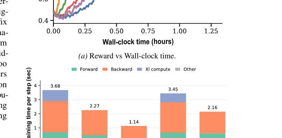
- Efficiency (Table 1, Figure 2): at the default budget , PS-PPO’s total per-step training time is s versus s for S-GRPO, s for DAPO, and s for DAPO-with-forking-tokens — a 33-45% reduction — even after paying the extra s overhead of computing the cutoff distribution itself. Peak GPU memory drops by 15-17%.
- Masking-only baselines (S-GRPO, DAPO-with-forking-tokens) don’t actually save compute, because they zero out the loss on some tokens but still run the forward/backward pass over the entire sequence — PS-PPO is the first method in this comparison set that actually shortens the computational graph itself (Figure 2(d)).
- Accuracy is preserved, not traded away: PS-PPO (Optimized) matches or slightly exceeds DAPO on 5 of 6 benchmarks per backbone (Table 2) — the optimized cutoff distribution is not just “cheaper,” it is measurably better at allocating the same expected compute budget than uniform or heuristic alternatives (Table 4 in the paper, discussed below).
- The efficiency advantage compounds with completion length: at tokens, PS-PPO is 2.8x faster than S-GRPO and 3.3x faster than DAPO per update step (Table 3), which matters increasingly as long chain-of-thought training becomes the norm.
- Boundary condition the paper is explicit about: all main experiments use binary correctness rewards; continuous-reward RLHF experiments (Appendix G, HH-RLHF/IMDB) are included but use a heuristic sigmoid-based binarization purely to feed the same uncertainty estimator, which is a real approximation layered on top of an approximation.
Prerequisites: What You Need to Know First
From a Language Model to an RLHF Policy
An autoregressive language model defines, token by token, a probability distribution over the next token given everything generated so far. In the RLHF setting, we treat the model as a policy: given a prompt sampled from some prompt distribution , the policy samples a completion token by token, where each token is drawn from and is the “state” — the prompt plus everything generated so far. After the full completion is produced, a reward function assigns a single scalar score to the entire completion — for math reasoning, typically if the final boxed answer matches the ground truth and otherwise.
The training goal is to adjust so that increases. This is a textbook reinforcement-learning objective, but with an unusual structure compared to classical RL: the “episode” is a single text generation, the “reward” typically arrives only once at the very end (sparse, terminal reward), and the “action space” at every step is the entire model vocabulary (often 100k+ tokens).
PPO’s Clipped Surrogate Objective
Proximal Policy Optimization (PPO) is the standard policy-gradient algorithm used to turn a scalar reward signal into a stable parameter update. Its central object is the per-token importance ratio:
which measures how much more (or less) likely the current policy is to produce the same token compared to the policy that actually generated the rollout. PPO’s training objective clips this ratio to prevent any single update from moving the policy too far from the data-generating distribution:
where is an estimated advantage — how much better token was than what the policy would typically do at state — and is a small clipping range (commonly 0.1-0.2). The classical formulation defines the advantage via a learned critic, , requiring a second value network trained alongside the policy.
Critic-Free Advantage Estimation (GRPO-style)
Training and maintaining a critic network at LLM scale is expensive and can itself be a source of instability (value-function mis-estimation compounds into noisy advantages). Critic-free methods like GRPO sidestep this entirely: for each prompt , sample a group of completions from the current policy, score each with the reward function, and use the group mean as the baseline:
Crucially, this advantage is a single scalar per completion, and it gets broadcast — assigned identically — to every timestep within that completion: for all . This is exactly the design choice PS-PPO’s efficiency argument targets: since the advantage carries zero token-level differentiation, backpropagating through the entire completion to apply this one number is potentially wasteful if most of the completion’s tokens contribute little extra information about whether the eventual reward will be 1 or 0.
Importance Sampling and Inclusion Probabilities
The mathematical tool PS-PPO relies on to truncate “safely” is a standard idea from survey sampling and Monte Carlo estimation called inclusion-probability reweighting (closely related to the Horvitz-Thompson estimator). If you want to estimate a sum but can only afford to observe a random subset of the terms, you can still get an unbiased estimate of the full sum by (a) including term with some known probability , and (b) dividing by whenever you do include it: . Because , each term’s contribution to the expectation is , exactly matching the full sum in expectation. The catch is variance: rarer inclusion (small ) means a larger multiplier when the term is included, so the estimator’s variance grows as inclusion probabilities shrink. PS-PPO’s whole design problem is choosing to control this variance-vs-compute trade-off, which is exactly the setup this background section is building toward.
A Closer Look at the Critic-Free Baseline Family (GRPO, Dr.GRPO, RLOO, DAPO)
Since the experiments compare against four closely related critic-free baselines, it is worth being precise about what actually distinguishes them from each other, since the paper’s efficiency argument applies identically to all of them (they all broadcast a scalar advantage across the full sequence) but their accuracy differs meaningfully in Table 2.
GRPO (Shao et al., 2024) is the foundational critic-free method: sample completions per prompt, use (note: normalized by the standard deviation of the group’s rewards, not just centered by the mean), then apply the standard PPO clip.
Dr.GRPO (Liu et al., 2025) identifies and corrects two subtle biases in vanilla GRPO: (a) dividing by the response length when averaging the per-token loss over a completion systematically biases the update toward favoring shorter completions (since a fixed total loss gets diluted more for longer responses), and (b) dividing the advantage by the group’s reward standard deviation introduces a difficulty-dependent scaling that inflates the effective learning rate on easy or hard prompts where the group’s rewards happen to have low variance. Dr.GRPO removes both normalizations.
RLOO (Ahmadian et al., 2024, “REINFORCE Leave-One-Out”) uses a slightly different baseline construction: for each sample , the baseline is the mean of the other samples’ rewards, , rather than the mean of all samples including itself — this removes a subtle self-correlation between a sample’s own reward and its own baseline, at the cost of a slightly noisier baseline estimate (since it uses one fewer sample).
DAPO (Yu et al., 2025) introduces several simultaneous changes: “Clip-Higher” (using a larger upper clip bound than lower clip bound, motivated by the same rare-token-under-penalization concern that later papers like DPPO analyze more rigorously), dynamic sampling (discarding prompts where all samples get the same reward, since these carry zero learning signal), token-level (rather than sample-level) loss averaging, and an overlong-response penalty. DAPO-with-forking-tokens further adds the entropy-based token-selection masking described above.
None of these four differences change the forward/backward compute profile of the baseline — they all still require processing every token of every completion — which is why PS-PPO’s efficiency comparison against all four in Table 1/Figure 2 shows a roughly consistent 33-45% speedup regardless of which specific critic-free baseline is used; the efficiency gain is orthogonal to which advantage-normalization scheme sits underneath it.
Convex Optimization and Lagrangian Duality (just enough to follow Appendix F)
A convex optimization problem minimizes a convex objective subject to constraints that define a convex feasible region; such problems have the property that any point satisfying the first-order (KKT) stationarity conditions is a global optimum, not just a local one. The Lagrangian relaxation technique folds an equality constraint (like “the sum of weighted by cost must equal budget ”) into the objective using a multiplier , turning a constrained problem into an unconstrained one whose stationary points can be found by simple calculus — differentiate with respect to each variable, set to zero, solve. PS-PPO’s core design problem (Equation 8 below) is convex in once you drop the monotonicity constraint, which is why a closed-form solution exists (derived in full in the Theory section below), and the monotonicity constraint is then restored via isotonic regression (Pool-Adjacent-Violators), a classic algorithm for finding the closest non-decreasing (or non-increasing) sequence to a given sequence under squared-error-like objectives.
Why Not Just Use a Learned Critic to Get Token-Level Signal?
A natural question at this point: if the problem is that broadcast advantages waste compute on uninformative tokens, why not simply go back to a learned critic, which would naturally assign different (token-level) advantages to different positions, presumably already down-weighting uninformative late tokens through the value function’s own learned structure? This is exactly the classical PPO design (Equation P1 above), and the paper’s introduction directly addresses why this is not the path taken: training a critic at LLM scale requires a second network (often as large as the policy itself, when done properly, though smaller critic architectures are sometimes used as a compute-saving compromise) trained alongside the policy, and mis-calibrated value estimates are themselves a well-documented source of training instability in LLM RL (cited to Kazemnejad et al., 2025 and Hao et al., 2025 in the paper’s introduction) — the field’s overall move toward critic-free methods (GRPO, RLOO, and their relatives) happened specifically to sidestep this cost and instability, and PS-PPO is explicitly positioned as compatible with that trend, not as an argument for reversing it. The trade-off PS-PPO makes instead is to keep the (simpler, more stable) broadcast advantage, but attack the computational symptom of broadcast advantages (full-sequence backpropagation) directly via principled truncation, rather than attacking the informational limitation (same advantage for every token) via a second network. This is a meaningfully different lever: PS-PPO does not make the advantage more informative per token, it makes spending compute on already-adequately-informed tokens optional.
The Compute Bottleneck PS-PPO Targets, In Concrete Terms
flowchart LR
    subgraph Rollout["Rollout stage (unchanged by PS-PPO)"]
        A["Sample prompt x"] --> B["Generate K completions via inference engine"]
        B --> C["Score each completion: R(x, o^(k))"]
        C --> D["Compute broadcast advantage A^(k) = R^(k) - mean(R)"]
    end
    subgraph Update["Gradient-update stage (this is where PS-PPO changes things)"]
        D --> E["Standard critic-free methods: forward+backward through ALL T tokens of every completion"]
        E --> F["Apply broadcast advantage to every token's log-prob gradient"]
    end
    style E fill:#ffdddd
Figure 1 (system overview, self-drawn): the reward-scoring and advantage-computation stages are identical across GRPO/DAPO/RLOO/PS-PPO — the divergence is entirely in the highlighted update stage, where a single broadcast scalar advantage is currently paying for a full-length forward/backward pass regardless of how much new information the later tokens actually carry.
The motivating data behind this diagram is Figure 1 of the paper itself, reproduced below:
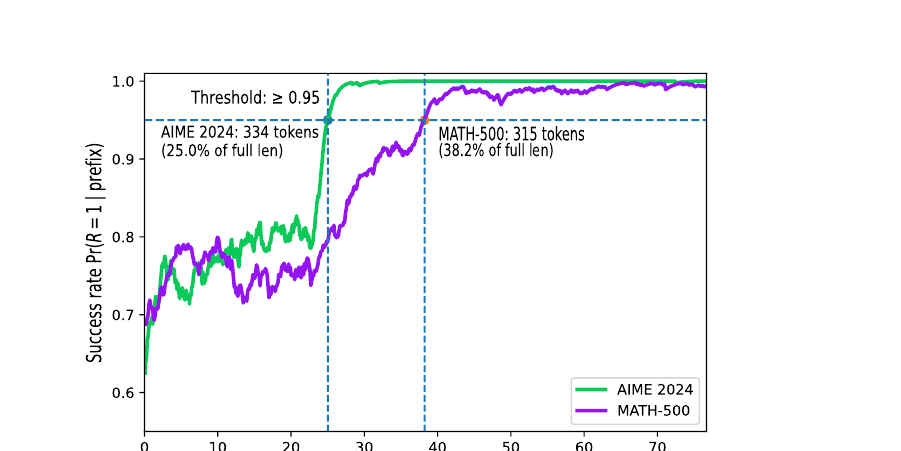
Reading this figure carefully: the y-axis, , is estimated empirically by taking a prefix of a given length, sampling 32 independent continuations from that prefix, and measuring what fraction end up correct. If this quantity is already close to 1 (or close to 0) at some prefix length, then continuing to generate — and, more importantly for PS-PPO, continuing to backpropagate through — the remaining tokens contributes little additional information about the eventual reward. The paper is careful to frame this correctly: this does not mean later tokens are useless for generation quality (a model that revises or self-corrects genuinely benefits from those tokens at inference time) — it means later tokens carry diminishing training signal once the outcome is already predictable, which is a narrower and more specific claim, quantified further in Appendix A’s “late-recovery analysis” (Table 6 in the paper): even at the 75% prefix mark, only 7.1-8.6% of finally correct completions still had prefix-conditioned success rate below 0.8, meaning “late recovery” (where a seemingly-doomed prefix turns into a correct final answer) is real but a minority pattern.
Theory Part 1: Deriving the Unbiased Truncated Estimator
The Truncation-and-Reweight Pipeline, Token by Token
Before the theory, it helps to see the actual data-flow this method inserts into an existing rollout: for each completion, tokens are classified into “kept, contributes full gradient (no reweighting)”, “kept past the point a naive fixed-length truncation would stop, but reweighted by ”, or “discarded entirely from the forward/backward pass” — and this classification is driven by the per-timestep survival probabilities derived in the rest of this section.
flowchart LR
    P["Prompt x, rollout produces tokens o_1 ... o_T"] --> D["Sample cutoff H ~ survival dist xi_1:T x"]
    D --> K1["Tokens t = 1..H: KEPT, gradient reweighted by 1/xi_t"]
    D --> K2["Tokens t = H+1..T: DISCARDED, no forward/backward compute spent"]
    K1 --> B["Truncated, reweighted gradient sum -> feeds PPO update (unbiased in expectation over H)"]
Figure: data-flow for a single completion under PS-PPO’s stochastic truncation — the cutoff is resampled independently per completion per training step, so across a batch, different completions are truncated at different lengths, and the reweighting on kept tokens is exactly what restores the full-sequence expectation despite discarding the tail.
Setting Up the Full-Sequence Update as a Sum
Start with the full-sequence critic-free policy-gradient update, summed over a group of completions per prompt:
This is exactly what GRPO/RLOO/DAPO already compute: for every token, multiply its per-token score function (the gradient of its log-probability) by the broadcast advantage, sum over all tokens and all completions in the group, and average. is the full-sequence “ground truth” gradient direction that PS-PPO wants to approximate with less compute.
Introducing the Random Cutoff and Reweighting
Now suppose each completion gets an independently sampled random cutoff , and we only backpropagate through tokens . Define the survival probabilities — the probability that the cutoff has not yet occurred by timestep , i.e., that token is retained. Note by convention (there is always at least a 1-token prefix) and (a survival function is necessarily non-increasing — you cannot become more likely to survive as time goes on). The naive truncated estimator, , is biased — it systematically underestimates because it silently drops the (possibly nonzero-in-expectation) contribution of tokens beyond the cutoff. The fix is the reweighted estimator:
Proving Unbiasedness, Step by Step
This is one of the paper’s two central theoretical results (Appendix B), and it’s worth walking through in full rather than taking on faith, since the entire method’s correctness rests on it. Define the inclusion indicator , so Equation 3 can be rewritten as a sum over all (not just up to the cutoff), since terms with automatically have :
Step 1 — the inclusion indicator’s expectation is exactly by construction: . This is just restating the definition of as a survival probability — it is not yet a proof of anything, but it is the load-bearing fact everything else depends on.
Step 2 — condition on the rollouts, only the cutoff is random: fix the prompt and the sampled trajectories (i.e., condition on everything except the cutoffs , which are sampled independently after the rollouts, from a distribution that can depend on but not on the specific tokens sampled — this independence is what the algorithm guarantees by construction, since is computed from prompt-level and batch-level statistics, not from a specific trajectory’s realized tokens beyond that). Under this conditioning, is a fixed, non-random quantity, and the only source of randomness left in Equation 4 is :
The middle step is the crux: can be pulled out of the conditional expectation (since it is fixed given the conditioning), leaving only for every single term — every term’s contribution collapses back to exactly , and summing recovers exactly, not approximately.
Step 3 — take the outer expectation over the rollouts themselves: since Equation 5 shows holds for every realization of the rollouts (this is a statement about the cutoff randomness alone, conditional on any fixed set of trajectories), taking the expectation of both sides over the rollout-sampling randomness gives trivially (since does not depend on the cutoff randomness at all). This closes the proof: the truncated, reweighted estimator has the exact same expectation as the full-sequence estimator, for any valid choice of survival probabilities — the choice of only ever affects variance, never bias.
Why does this matter practically? It means PS-PPO is not making an approximation trade-off between “faster” and “correct” — it is making a trade-off between “faster” and “variance,” which is a fundamentally more benign trade-off, because variance can be controlled by choosing well (which is exactly the next section’s job), whereas bias generally cannot be fixed after the fact.
Theory Part 2: Designing the Cutoff Distribution as a Convex Optimization Problem
Why Not Just Pick Arbitrarily?
The unbiasedness proof above holds for any monotone, valid survival sequence — including terrible choices like for all (no truncation, no savings) or decaying so fast that almost nothing is retained (huge compute savings, but enormous variance from the reweighting blowing up on the rare retained tokens). The paper’s actual technical contribution is choosing well — specifically, to minimize the extra variance the truncation introduces, subject to spending only a fixed expected amount of compute.
Deriving the Tractable Variance Surrogate (Equation 4 in the paper)
The exact variance of induced by the cutoff randomness (i.e., , a scalar trace/diagonal summary of the full covariance matrix) would in principle require reasoning about cross-timestep correlations, because the same trajectory’s tokens at nearby positions are autoregressively dependent. The paper makes this tractable by keeping only the diagonal (per-timestep) variance terms and dropping cross-timestep covariances — a deliberate, explicitly-acknowledged approximation, justified because keeping the cross-terms would couple the design variables across timesteps and destroy the clean per-timestep structure that makes the optimization solvable in closed form.
Here is the derivation in full (Appendix C), reproduced with every intermediate step spelled out:
Step 1. Write explicitly using the fact that (shown above):
Step 2. Because cutoffs are sampled independently across the completions, cross-completion covariance terms vanish, and the trace-of-covariance surrogate becomes:
where a single generic pair stands in for any one of the completions (dropping the superscript for readability), and the cross-timestep covariance terms within a single trajectory are the ones being discarded by the diagonal-only surrogate.
Step 3. Compute the inner expectation explicitly. Since is a Bernoulli variable,
which follows from expanding the two-outcome expectation directly: with probability the term is , and with probability the indicator is 0 so the term is ; the algebra confirms the simplified form.
Step 4. Substitute back and take the expectation over the rollouts to define (the expected squared norm of the per-timestep gradient contribution, over the randomness of which token gets sampled and what its advantage turns out to be), giving the paper’s Equation 4:
Reading this formula intuitively: the extra variance from truncation is a sum over timesteps of “how much this timestep’s gradient matters” () times “how much reweighting penalty this timestep pays for being included with low probability” (, which blows up as and vanishes as ). This immediately suggests the right design principle: give high inclusion probability to timesteps with large (important gradients), and allow low inclusion probability for timesteps with small (unimportant gradients) — exactly the intuition Figure 1’s empirical curve supports, since late tokens in an already-predictable trajectory should have small .
The Full Design Problem and Its Closed-Form Solution
Minimizing Equation 4 with respect to , subject to an expected-compute budget (this expression is exactly , the expected retained prefix length — a standard identity for non-negative integer random variables, , which after an Abel-summation-by-parts rearrangement becomes the telescoping form used here) and the survival-monotonicity constraint , is equivalent to the simpler problem:
Solving the relaxed (non-monotone) version first. Temporarily drop the monotonicity constraint and consider the simpler equality-constrained problem s.t. (approximating the budget constraint in its simpler additive form — the paper’s Appendix F works with this equivalent formulation directly). Form the Lagrangian:
Taking the partial derivative with respect to a single and setting it to zero:
Substituting this form back into the budget constraint gives , i.e., , so the closed-form unconstrained-monotonicity solution is:
Reading this formula: the optimal inclusion probability at timestep is proportional to the square root of that timestep’s gradient-importance weight — not linearly proportional. This square-root relationship falls directly out of the term in the objective (a hyperbolic penalty for small ) balanced against the linear budget constraint — it is the same square-root allocation rule that shows up throughout stratified-sampling theory (Neyman allocation) whenever you are minimizing a sum of -type terms under a linear budget.
Restoring monotonicity via blockwise pooling. Equation 6 does not generally produce a non-increasing sequence — (gradient importance) can go up and down non-monotonically across timesteps, so can too, even though is required to be non-increasing (since it represents a survival probability). The paper resolves this the standard way isotonic regression problems are resolved: partition into contiguous blocks, force to be constant within each block, and solve the same Lagrangian problem at the block level. For a block of length with aggregated weight , the identical derivation (replacing “per-timestep” with “per-block”) gives:
If the block scores already happen to be non-increasing, this blockwise solution is already the correct monotone global optimum. If not — some later block scores higher than an earlier one, which would require a non-monotone survival sequence — the Pool-Adjacent-Violators (PAV) algorithm merges the two violating adjacent blocks into one larger block (recomputing and for the merged block) and repeats until the sequence of block scores is non-increasing. PAV is a well-known, exactly-optimal, -amortized algorithm for isotonic regression, so this step adds negligible overhead relative to the forward/backward savings being sought.
Pseudocode for the full budgeted-monotone-cutoff computation:
Input: per-timestep weights w_1, ..., w_T (from the forward-only proxy, see below);
       budget B
1. Compute unconstrained scores: score_t = sqrt(w_t) for each t = 1..T
2. Initialize each timestep as its own singleton block: blocks = [{t}: t=1..T]
   with block_score[t] = score_t, block_length[t] = 1, block_weight[t] = w_t
3. While there exist adjacent blocks (m, m+1) with block_score[m] < block_score[m+1]:
       merge blocks m and m+1 into a single block m':
           block_length[m'] = block_length[m] + block_length[m+1]
           block_weight[m'] = block_weight[m] + block_weight[m+1]
           block_score[m']  = sqrt(block_weight[m'] / block_length[m'])
       (this is exactly the Pool-Adjacent-Violators merge step)
4. After convergence, block_score is non-increasing across the final blocks
5. Assign xi_t = B * block_score[block(t)] / sum_j(block_length[j] * block_score[j])
   for every t in block j -- this is the final xi_t^* used for sampling cutoffs
Output: monotone cutoff probabilities xi_1 >= xi_2 >= ... >= xi_T > 0
Where Does the Budget Constraint’s Telescoping Form Come From?
The budget constraint used in Equation 5, , looks less intuitive on first read than the simpler additive form used in the Lagrangian derivation above — it is worth showing these are the same quantity, since the equivalence is only asserted, not shown, in the paper’s main text. Start from the standard identity for the expectation of a non-negative integer-valued random variable with support on : (this identity itself follows from writing and taking expectations, swapping sum and expectation by linearity). Now apply summation by parts (the discrete analogue of integration by parts) to rewrite this sum in the “telescoping” form: define (with ), which is the probability mass as used in the worked numeric example above. Then (since , a telescoping sum recovering from the tail of the mass function), and swapping the order of the double sum, — which is exactly the constraint’s telescoping form. So the two forms of the budget constraint, and , are algebraically identical restatements of ""; the paper’s main text uses the second form because it makes the connection to a discretized “expected retained length” more explicit when is thought of via its probability mass function rather than its survival function, but the Lagrangian derivation is most transparent using the first (additive) form, which is why this review used that form when deriving the closed-form solution above.
Why Square-Root Allocation, Not Linear or Equal Allocation? A Numeric Comparison
It is worth checking, with actual numbers, why the derivation produces rather than the perhaps more intuitive-sounding (linear allocation) or for all (equal allocation). Take a toy example with just two timesteps, (very important) and (unimportant), and a budget (i.e., we can afford to fully retain, in expectation, one token total across the two).
Equal allocation would give , spending the budget identically regardless of importance — clearly wasteful, since is 9x more important than but gets no extra inclusion probability.
Linear allocation () would give , . Plugging into the true objective being minimized, .
Square-root allocation (the actual derived optimum) gives , (since , and ). Plugging into the same objective: — strictly lower than linear allocation’s 16 < 20, confirming the square-root rule genuinely outperforms the naive linear-proportional intuition on this objective, even though linear allocation seems like the more “obvious” way to make important timesteps more likely to be included. The intuitive reason square-root wins: the objective has a convex, accelerating penalty for small (it blows up like , not linearly), so the marginal benefit of moving away from an already-small value is larger than the marginal benefit of moving an already-large even higher — square-root allocation strikes the balance point where the marginal penalty (from the stationarity condition ) is exactly equalized across timesteps, which is what the Lagrangian derivation formalizes and this numeric check confirms concretely.
Why the Convexity/Monotonicity Machinery Is Worth the Trouble (Design Choice Discussion)
It is worth pausing to ask: why not skip all this optimization and just use something simple, like a fixed decay schedule ? The paper actually tests exactly this as a baseline — “PS-PPO (Time-Prior)” — and Table 4/Figure 3 in the paper show it performs no better than uniform-random cutoffs. The reason, made clear by the derivation above, is that a fixed decay schedule assumes the shape of “how quickly a trajectory becomes predictable” is the same for every prompt, but Figure 1 itself shows this is false even between two benchmarks (AIME 2024 stabilizes at 25% of length, MATH-500 at 38%) — let alone between individual problems within a benchmark. The optimized, prompt-conditioned derived above is specifically not a fixed function of alone; it depends on through , which is re-estimated from the current batch’s rollouts for that specific prompt. This is the “what if not” answer to why the heavier optimization machinery earns its keep: a context-independent heuristic cannot adapt to the fact that “the point at which a trajectory becomes predictable” is itself a property of the specific problem being solved, not a universal constant of trajectory length.
A Worked PAV Example Where Merging Is Actually Needed
The numeric example given earlier in this review (Step 0-4 under “A Fully Worked Numeric Example”) was deliberately constructed so that the raw scores came out already monotone, meaning PAV had nothing to do. Since PAV is the one genuinely new algorithmic component this paper introduces relative to a standard Lagrangian relaxation, it is worth working through a small example where a monotonicity violation actually occurs and must be repaired.
Suppose with raw weights , , , — notice , so the unconstrained scores are not non-increasing (they go up from to before coming back down), which would violate the required survival-function monotonicity if used directly as .
PAV Step 1 — initialize singleton blocks. Each timestep starts as its own block: block scores are , block lengths are all 1, block weights equal the raw : .
PAV Step 2 — scan for violations. Comparing adjacent blocks left to right: block 1 (score 1) vs block 2 (score 3) — violation, since but we need non-increasing order. Merge blocks 1 and 2: new block has length , weight , and score .
PAV Step 3 — re-check after merging. Blocks are now , , . Check block 1 (2.236) vs block 2 (2.0): — OK, no violation. Check block 2 (2.0) vs block 3 (1.0): — OK, no violation. The sequence of block scores is now non-increasing, so PAV terminates.
PAV Step 4 — assign final . With budget (say), the normalizing denominator is . Then: (both timesteps in the merged block get the same , since PAV forces them to be pooled together), , .
Sanity checks. Monotonicity: — non-increasing (with equality inside the merged block), satisfying the survival-function requirement. Budget: — correct up to rounding.
The interpretation worth pausing on: timestep 1, which individually had the smallest raw weight (), ends up with the same inclusion probability as timestep 2, which had the largest raw weight () — because the monotonicity constraint forces them into the same block once a violation is detected. This is the real-world cost of imposing monotonicity: some individual timesteps get “pooled” with neighbors and lose their ability to have a uniquely-tailored inclusion probability, precisely in proportion to how badly the raw importance signal violates the required non-increasing shape. This is also, incidentally, exactly why the paper’s Figure 1 motivation (importance roughly decreasing over the course of a trajectory, at least in aggregate) matters for PAV not degrading the solution too much in practice — if raw importance were highly non-monotonic in a real training run, PAV would end up pooling large portions of the trajectory together, diluting the fine-grained resolution the optimization is trying to achieve.
Making the Weights Computable Without a Backward Pass
The Forward-Only Score-Norm Proxy
There is a chicken-and-egg problem lurking in the design above: computing requires the full gradient norm across all of — which requires exactly the full backward pass PS-PPO is trying to avoid, for every candidate cutoff decision. The paper’s resolution is to approximate this using only the output head’s contribution to the gradient, which is computable from forward-pass quantities alone.
Derivation of the closed-form output-head score (Appendix D). For a standard softmax output head, , , where is the last-layer hidden state (already available from the forward pass). For the actually-sampled token , the gradient of its log-probability with respect to the output-head weight matrix has the well-known closed form:
where is the one-hot vector for the sampled token. This is the standard softmax-cross-entropy gradient identity: the gradient with respect to the logits is exactly “one-hot minus predicted distribution,” and it requires no backward pass to derive because it is a closed-form function of quantities the forward pass already produces () and the sampled token identity (). Taking the squared Frobenius norm:
The second equality expands , using that is one-hot () and (picking out the sampled-token probability). Combining gives the paper’s proxy:
Handling the seemingly-expensive term efficiently. Computing naively requires materializing the entire softmax distribution over the (100k+ token) vocabulary and squaring every entry — not prohibitive, but avoidable with a neat log-sum-exp trick shown in Appendix D: define (the standard log-partition function, already computed for the token log-probability) and (a second log-sum-exp over doubled logits), then — derived directly from . Both and are cheap scalar reductions over the logits, computable in the same forward pass that already computes the token log-probability — no backward pass, no explicit full-vocabulary elementwise squaring-and-summing loop needed beyond a single log-sum-exp variant.
Why this proxy is defensible, not just convenient. Since is a strict subset of all trainable parameters , and squared norms decompose additively across independent parameter blocks, — the output-head norm is always a lower bound on the true full-parameter score norm, not an unrelated correlate. The paper additionally validates empirically that this lower bound tracks the true norm closely rather than loosely:
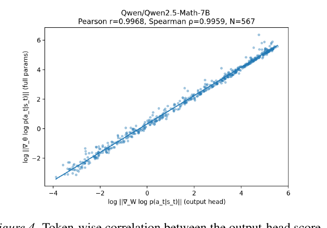
A Pearson correlation of 0.9968 on a log-log plot is a strong empirical validation — it means that even though the output-head norm is provably only a lower bound and not an exact match, the relative ordering of “which tokens have large gradients” is almost perfectly preserved, which is exactly the property the cutoff-design optimization actually needs (it only needs to correctly rank timesteps by importance, not match their absolute gradient magnitudes).
The Reward-Uncertainty Term and Its Upper-Bound Derivation
The other ingredient the weight needs, once the advantage-squared factor enters via the law of total expectation and a mean-field approximation, is an estimate of — how uncertain the eventual reward still is, given the prefix state . For binary rewards this is a variance of a Bernoulli variable, and the paper derives a computable upper bound (Appendix E) rather than trying to estimate the variance directly (which would require many suffix rollouts per prefix — exactly the expensive experiment used only for the validation Figure 1, not something affordable at every training step).
Step 1 — a generic bound on Bernoulli variance. For with , the variance is , and a standard fact is (variance is at most the smaller of the two probabilities — true because when , and symmetric otherwise). Using the identity with gives .
Step 2 — take expectation over the random prefix state and rewrite the absolute-value term as a total-variation-like quantity. Taking of both sides, and expanding using , a short algebraic rewrite (Equation 20 in the paper’s Appendix E) turns the expectation into an -distance between two joint distributions over (prefix state, reward):
Step 3 — map prefix states to next-token distributions to make this estimable. The distribution over prefix states is not directly convenient to estimate during training (it lives in an enormous state space), so the paper uses the triangle inequality to further bound this by a quantity expressed in terms of the next-token distribution under the old policy — something that already has a natural empirical estimator from the rollout batch:
where is the empirical success rate for the prompt (estimated from the -completion group), and are the state-averaged next-token distributions under the old policy, computed separately over the successful and unsuccessful rollouts in the group. The final guarantee, , is a genuine mathematical upper bound (not a heuristic approximation with unknown error direction) — the chain of inequalities above (Bernoulli variance bound triangle inequality on the state distribution next-token-distribution rewriting) is monotone throughout, so can only overestimate, never underestimate, the true reward uncertainty. In practice, , , and are all estimated empirically from the same rollouts the group-relative advantage already uses — no extra rollouts, no auxiliary reward-uncertainty model.
Unpacking the Mean-Field Factorization Step
One step in the derivation deserves a slower look than the paper affords it: the move from (Appendix D’s target quantity) to the factored form used in Equation 7. In general, the expectation of a product of two random quantities is not the product of their expectations unless the quantities are independent (or the factorization is otherwise justified) — only holds exactly when , or approximately when their correlation is small. Here, (essentially the squared advantage magnitude, which depends on the full trajectory’s eventual reward) and (the score-norm proxy, which depends on the specific prefix state and sampled token at step ) are generally not independent — a prefix state that makes the eventual reward more or less certain plausibly also correlates with the confidence (and hence the score-norm proxy) of the model’s own next-token distribution at that state. The paper’s derivation handles this via what it calls a “mean-field approximation” (an approximation that ignores such cross-correlations, treating the two factors as if they varied independently even though they may not), explicitly flagged as an approximation rather than an identity. This is one more link in the chain of approximations this method stacks (diagonal-variance surrogate forward-only score-norm proxy reward-uncertainty upper bound mean-field factorization), and while each individual approximation is reasonably motivated and, where possible, bounded (the reward-uncertainty piece is a provable upper bound; the diagonal-variance and mean-field pieces are not shown to be bounds, only “reasonable” approximations), the paper does not report an ablation quantifying how much cumulative error this specific chain of approximations introduces relative to using the exact (expensive, backward-pass-requiring, multi-suffix-rollout-requiring) quantities at every stage. This is consistent with this review’s critical-assessment point above about the absence of a controlled comparison against the exact score norm, but it is worth stating explicitly as a second, distinct instance of the same broader pattern: a real, useful method built from several individually-reasonable-but-unverified approximations layered together, where the overall empirical validation (Table 1/2’s efficiency-and-accuracy numbers) is the only evidence that the accumulated approximation error stays small in practice, rather than there being a decomposed accounting of where the error budget actually goes.
Why this matters as a design choice, not just a technical footnote: an alternative, simpler design would be to estimate directly by sampling multiple suffix continuations from each prefix during training (exactly what Figure 1’s validation experiment does) — but that would cost 32x additional rollouts per training step, defeating the entire purpose of a compute-saving method. The derivation above trades a small amount of estimation tightness (the bound is provably loose in general, since two levels of inequality relaxation are stacked) for the ability to compute the signal essentially for free from data that is already being collected for the advantage estimate.
Putting It Together: The Final Optimization Problem and Algorithm
Combining the score-norm proxy (aggregated over the batch as ) with the reward-uncertainty upper bound , the paper defines the final per-timestep design weight as their product, , and solves:
which, per the derivation walked through above, is solved by the Lagrangian closed form followed by PAV to restore monotonicity.
Algorithm 1 (Prefix-Sampling PPO), reproduced and annotated line by line:
Require: policy pi_theta; prompt distribution p_Q; reward function R;
         max training steps N; old-policy refresh period F;
         group size K; max completion length T; compute budget B.

 1: Initialize theta, and set theta_old <- theta.
 2: for iteration n = 1 to N do
 3:     Sample a prompt x ~ p_Q.
              # identical to any critic-free RLHF method
 4:     Sample K completions {tau^(i)} from pi_theta_old(. | x).
              # identical -- this is the rollout stage PS-PPO does not touch
 5:     Compute terminal rewards {R^(i)}.
              # identical -- the reward function is untouched
 6:     Compute critic-free advantages {A_hat^(i)} using the within-prompt baseline.
              # identical -- e.g. GRPO-style group-relative advantage
 7:     Compute per-timestep proxies {u_t(x), gamma_bar_t(x,t)} from {(tau^(i), R^(i))}.
              # NEW: forward-only score-norm proxy (Eq. 6) + reward-uncertainty upper bound (Eq. 7),
              #      both estimated from the SAME K rollouts already sampled in step 4 -- no extra data needed
 8:     Set cutoff weights w_t(x) <- gamma_bar_t(x,t) * u_t(x) for t = 1..T.
              # NEW: combine the two proxies into the design weight
 9:     Compute monotone cutoff probabilities xi_1:T by solving the budgeted design problem (Eq. 8).
              # NEW: closed-form sqrt(w_t) allocation + PAV for monotonicity (see pseudocode above)
10:     Sample cutoffs {H^(i)} from the cutoff distribution induced by xi_1:T.
              # NEW: one random draw per completion
11:     During the update pass, backpropagate only through tokens t <= H^(i)
              and reweight token losses by 1/xi_t.
              # NEW: this is the actual compute saving -- shorter backward graphs
12:     Update theta using PPO with the truncated, reweighted gradient estimator (Eq. 9 in the paper).
              # identical PPO update mechanics, just applied to fewer tokens
13:     if n mod F == 0 then
14:         theta_old <- theta
              # identical -- standard old-policy refresh schedule
15:     end if
16: end for
17: return optimized policy pi_theta.
Reading the annotations together, the algorithm’s actual footprint on an existing critic-free RLHF pipeline is confined to steps 7 through 11 — everything about rollout generation, reward scoring, advantage computation, and the PPO update rule itself is unchanged. This is exactly why the paper can report the efficiency numbers below as an almost drop-in replacement rather than requiring a redesigned training system.
Why Truncating the Forward Pass Also Saves Memory, Not Just Time
It is worth being explicit about the mechanism behind the reported 15-17% peak-memory reduction (mentioned in Table 1’s surrounding text), since “shorter backward pass” and “less memory” are related but not identical claims, and conflating them would miss part of the picture.
During a standard transformer forward pass, every layer’s intermediate activations (attention scores, feedforward hidden states, layer-normalized outputs, etc.) must be retained in memory until the backward pass consumes them to compute gradients — this is the well-known activation-memory bottleneck that gradient checkpointing and similar techniques target. The memory cost of storing these activations scales roughly linearly with sequence length: a sequence of length requires storing on the order of times as much activation memory as a sequence of length 1 (per layer, per batch element), because the attention mechanism and every subsequent per-token computation must be preserved for every one of the positions.
When PS-PPO truncates a completion to its sampled cutoff before the forward pass runs (rather than running the forward pass over all tokens and discarding some afterward), the activation memory required is proportional to , not . Averaged over a batch of completions with varying (randomly sampled) cutoffs, the expected activation memory scales with rather than with the (typically much larger) — this is the direct mechanistic explanation for why Figure 2(c)‘s peak-GPU-memory panel shows PS-PPO using consistently less memory than the full-sequence baselines throughout training, not just at the very end.
This is also precisely why the masking-only baselines (S-GRPO, DAPO-with-forking-tokens) do not show a comparable memory reduction: masking the loss after the fact does nothing to reduce the activation memory that had to be allocated and retained during the full-length forward pass in the first place — by the time the mask is applied, the memory has already been spent. This is the same underlying mechanism (truncating the computational graph itself, versus post-hoc masking a full-length graph) that explains both the time savings (Table 1) and the memory savings (Figure 2(c)) — they are two symptoms of the same root cause, not two independent design wins.
Experiments: What the Numbers Actually Show
Efficiency: Where the Time and Memory Savings Come From

Panel (d) is the figure that makes the paper’s central efficiency claim legible in one glance: for S-GRPO and DAPO-with-forking-tokens, the number of tokens with non-zero loss (light bars) is meaningfully smaller than the number of tokens actually backpropagated through (dark bars) — these methods mask which tokens contribute gradient, but the forward and backward passes still have to run over the full, unmasked sequence length to produce those masked-out zero-loss values in the first place. PS-PPO’s bars are the only pair where both loss-tokens and backpropagated-tokens shrink together, because the truncation happens before the forward pass even starts (the sequence fed to the network is shorter), not as a post-hoc masking of an already-computed loss tensor. This is precisely the “why this design choice, and what would the obvious alternative do” discussion clause 15 asks for: the obvious alternative to PS-PPO’s approach is exactly what S-GRPO and DAPO-with-forking-tokens already do (compute everything, then zero out unwanted contributions), and the reason that alternative saves little wall-clock time is that modern accelerator hardware pays for the forward/backward matrix multiplications regardless of whether their outputs are subsequently zeroed by a loss mask — there is no way to recover the FLOPs already spent.

Breaking Table 1 down term by term: PS-PPO’s forward cost (0.32s) is already lower than every baseline’s forward cost (0.82-1.12s), which makes sense since PS-PPO’s sequences are shorter before the forward pass runs at all — the truncation is not merely a backward-pass optimization. The backward cost (1.01s) is likewise the lowest of the four. The one place PS-PPO pays extra is the “Computing ” column (0.43s, versus N/A for methods that don’t do prompt-conditioned cutoff design at all) — and the paper’s honest accounting keeps this cost in the total rather than hiding it, showing that even after paying it, the net remains a clear win.
Accuracy: Does the Efficiency Come at a Cost?
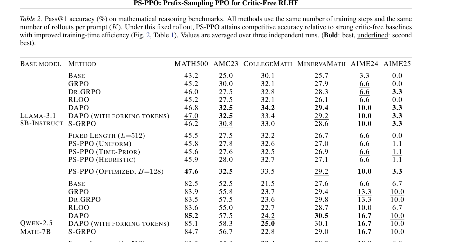
The critical comparison here is between “PS-PPO (Optimized, B=128)” and the strongest baselines. On Llama-3.1-8B-Instruct, PS-PPO (Optimized) achieves the single best score on MATH500 (47.6, beating DAPO-with-forking-tokens’ 47.0) and AMC23 (32.5, tied with DAPO and DAPO-with-forking-tokens), and is competitive (not best, not worst) on the remaining four benchmarks. On Qwen2.5-Math-7B, PS-PPO (Optimized) achieves the best AIME25 score (13.3, versus 10.0 for the next-best methods) while remaining competitive elsewhere. Just as informative is the comparison within the PS-PPO family: “PS-PPO (Uniform),” “PS-PPO (Time-Prior),” and “PS-PPO (Heuristic)” all underperform “PS-PPO (Optimized)” by a consistent, non-trivial margin across almost every benchmark and both base models — this isolates that the gain is specifically attributable to solving the convex design problem, not merely to “truncating training somehow.” A skeptical reader’s natural question — “maybe any reasonable truncation scheme would have worked equally well, and all this optimization machinery is overkill” — is directly addressed by this internal ablation, and the answer the data gives is no.
Scaling with Completion Length
As chain-of-thought training moves toward longer completions, the paper directly tests whether PS-PPO’s advantage grows or shrinks with completion length, sweeping :
| Method | Time/step (s) | Avg. accuracy (MATH500, AIME24, AIME25) | |
|---|---|---|---|
| 1024 | PS-PPO | 1.77 ± 0.02 | 38.3 |
| 1024 | S-GRPO | 2.66 ± 0.01 | 37.1 |
| 1024 | DAPO | 3.23 ± 0.01 | 37.3 |
| 4096 | PS-PPO | 2.39 ± 0.04 | 42.1 |
| 4096 | S-GRPO | 6.70 ± 0.04 | 39.7 |
| 4096 | DAPO | 7.78 ± 0.04 | 42.2 |
Figure 3 (paper Table 3, restated as a comparison table): at , PS-PPO’s time-per-step (2.39s) is 2.8x faster than S-GRPO (6.70s) and 3.3x faster than DAPO (7.78s), while its average accuracy (42.1) is within noise of DAPO’s (42.2) and clearly ahead of S-GRPO’s (39.7).
The design-relevant observation here is how little PS-PPO’s time-per-step grows as triples (1.77s 2.39s, a 35% increase) compared to how much the baselines’ time-per-step grows (DAPO: 3.23s 7.78s, a 141% increase) — this is the direct, mechanistic consequence of PS-PPO’s expected backpropagated length being governed by the budget rather than by itself: as completions get longer, PS-PPO simply truncates a larger fraction of each one, while the baselines’ backward pass cost scales roughly linearly with the full completion length regardless of how predictable the outcome became partway through.
Isolating the Cutoff Strategy Under a Matched Budget
To answer the specific question “is the gain from less compute per step, or from smarter allocation of the same compute,” the paper runs a controlled comparison at matched expected backpropagated length (, , so uniform cutoff gives by construction, matching the other strategies’ budget exactly):
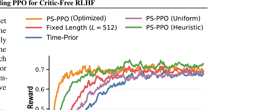
This pair of figures directly answers the “what would the obvious alternative do” question for the cutoff-design choice: if you fix the amount of compute spent (same expected tokens backpropagated) but vary where that compute is spent (which timesteps get included), the Optimized/Heuristic strategies reach the same final reward substantially faster in wall-clock time than Uniform or Time-Prior — meaning the gain is not simply “PS-PPO spends less compute” (that comparison is Table 1/Figure 2), it is also “for a fixed compute budget, PS-PPO’s specific allocation of that budget across timesteps is measurably better than naive alternatives” (this comparison). The paper is careful to note Time-Prior’s failure specifically: simply favoring earlier timesteps (without conditioning on the actual reward-uncertainty signal) performs no better than pure Uniform — confirming that the design principle (allocate probability mass according to , not according to raw position ) is doing the real work, not some generic “recency bias toward early tokens.”
Hyperparameter Sensitivity: Budget and Group Size
The paper reports two ablations worth summarizing concisely (Tables 4 and 5 in the paper): sweeping the budget shows accuracy rising from 34.0 (average) at to 37.9 at , then essentially plateauing (37.5 at , 37.8 at ) while training time per step keeps climbing linearly (1.15s 1.77s 2.01s 2.56s) — this identifies a clear diminishing-returns knee around , which the paper adopts as its default. Sweeping the group size shows a similar but distinct pattern: accuracy keeps improving all the way to (34.2 38.5), but the paper argues is the practical sweet spot because it achieves performance close to (37.9 vs 38.5) at substantially lower per-step training cost (1.77s vs 2.24s), and — a subtler point worth surfacing explicitly — because directly affects the quality of the estimate itself: with small , the successful/unsuccessful rollout split used to estimate often has too few examples on one side (or all rollouts land on the same side, a fully “degenerate” batch with zero learning signal regardless of cutoff strategy), making noisy and pushing the resulting cutoff distribution toward an uninformative near-uniform shape — a second-order interaction between and the cutoff-design machinery that is easy to miss if you only look at the headline accuracy numbers.
Quick Reference: When Does PS-PPO’s Advantage Matter Most?
A short decision-oriented summary of when the mechanism this paper introduces is likely to matter, versus when it may not be worth the added implementation complexity:
| Situation | Relevance of PS-PPO |
|---|---|
| Long chain-of-thought RL training (thousands of tokens per completion) | high — Table 3 shows the speedup advantage over masking-only baselines grows from roughly 1.5x at to 2.8-3.3x at , and the paper’s own motivation suggests this trend should continue at even longer lengths |
| Binary/verifiable rewards (math, code correctness, exact-match tasks) | high — this is the setting the reward-uncertainty proxy was natively derived for |
| Continuous reward-model-based RLHF (general helpfulness/harmlessness) | moderate — works per Appendix G, but relies on an extra sigmoid-binarization approximation layered on top of the native derivation |
| Rollout/generation dominates total training wall-clock time (e.g., very slow inference engine, small model but expensive sampling) | lower — PS-PPO only touches the gradient-update stage, not rollout; the relative benefit shrinks if rollout is already the bottleneck |
| Short completions (a few dozen tokens, e.g., single-sentence classification-style rewards) | low — little redundant suffix to truncate in the first place, so the method’s core motivation (Figure 1’s prefix-predictability curve) is less applicable |
| Already using a masking-only token-selective method (S-GRPO, DAPO-with-forking-tokens) | high — Figure 2(d) shows these methods reduce loss-tokens but not backpropagated-tokens; switching to PS-PPO’s actual-truncation approach would likely realize further savings without sacrificing the token-selection benefit already obtained |
| Using an actor-critic method with a learned token-level critic (not critic-free) | untested — the paper’s specific derivation assumes broadcast (constant-across-) advantages; adapting to token-varying advantages is flagged above as a natural but unexplored extension |
Model Scale and Experimental Configuration Summary
For quick reference, here is every model and configuration used across the paper’s experiments:
| Model | Role | Used in |
|---|---|---|
| Llama-3.1-8B-Instruct | dense, 8B | main mathematical-reasoning experiments (Table 2), completion-length scaling (Table 3), cutoff-strategy ablation (Figure 3) |
| Qwen2.5-Math-7B | dense, 7B, math-specialized | main mathematical-reasoning experiments (Table 2), budget/rollout-count ablations (Tables 4-5), score-norm-proxy validation (Figure 4) |
| Qwen2.5-3B-Instruct | dense, 3B | continuous-reward generation tasks (Appendix G, Tables 7-8) |
| lvwerra/gpt2-imdb | reward model | Positive Generation task (IMDB sentiment reward) |
| weqweasdas/RM-Gemma-2B | reward model | Helpful Assistant task (HH-RLHF-based reward) |
| Configuration axis | Values tested |
|---|---|
| Budget | 64, 128 (default), 256, 512 |
| Group size | 2, 4, 8 (default), 16 |
| Max completion length | 1024 (default main setting), 2048, 4096 |
| Top- for reward-uncertainty estimation | 16 (default, used throughout) |
| Training epochs | up to 3 |
| PPO clip | 0.1 |
| Learning rate | |
| Hardware | 8 x NVIDIA A100 GPUs |
Limitations and Boundary Conditions the Paper Acknowledges
- All main experiments use binary correctness rewards. The continuous-reward RLHF experiments (Appendix G, HH-RLHF and IMDB-positive-generation with learned reward models) require an ad hoc sigmoid-based binarization of the reward, , purely to plug into the estimator, which was derived specifically for the binary case. This is explicitly flagged as reusing an estimator outside its original derivation’s assumptions.
- The diagonal/trace variance surrogate discards cross-timestep covariance. The paper is upfront that the exact variance expansion contains cross-timestep covariance terms from autoregressive dependence, and that keeping them would couple the across timesteps in a way that destroys the closed-form solvability — but this means the “optimal” is optimal only with respect to the tractable surrogate, not with respect to the true variance.
- The forward-only score-norm proxy is a strict lower bound on the true gradient norm, validated only on Qwen2.5-Math-7B in the correlation study (Figure 4); it is not shown to hold with equal fidelity for architectures with substantially different output-head designs (e.g., tied embeddings, mixture-of-experts routing at the final layer) or at different scales.
- The reward-uncertainty upper bound is a two-inequality-deep relaxation (Bernoulli-variance bound, then triangle-inequality state-to-next-token mapping) — the paper proves it is a valid upper bound but does not characterize how loose it typically is in practice, only that it is estimable cheaply.
- All main math-reasoning experiments use one dataset family (MATH, evaluated on MATH500/AMC23/CollegeMath/MinervaMath/AIME24/AIME25) and two model sizes (7-8B). Generalization to substantially larger models (70B+) or to non-mathematical domains where prefix-predictability may behave differently (e.g., open-ended creative writing, multi-turn dialogue with delayed rewards) is not empirically tested.
- Late-recovery is acknowledged but not eliminated. Appendix A’s own analysis shows 7-9% of finally-correct completions still have prefix-conditioned success rate below 0.8 even at the 75% prefix mark — the method’s stochastic (rather than deterministic) truncation is specifically designed to hedge against this by still allowing later cutoffs with nonzero probability, but the paper does not report how much accuracy would be lost under an even more aggressive budget that effectively eliminated this hedge.
Critical Assessment: Weaknesses & Improvements
Weaknesses and unconvincing evidence. First, the headline “33-45% training-time reduction” and “15-17% memory reduction” figures (Table 1, Figure 2) are measured excluding rollout/generation time — this is explicitly stated by the paper, but it means the reported speedup applies only to the gradient-update stage, not to the wall-clock cost of an entire RLHF training run, in which rollout/generation (running the inference engine to sample completions) is often the dominant cost, especially for long chain-of-thought completions. The paper never reports an end-to-end wall-clock comparison that includes rollout time, which would give a much more conservative (and practically relevant) picture of the actual speedup a practitioner should expect. Second, the accuracy comparison in Table 2 shows PS-PPO (Optimized) winning or tying on only a subset of the 12 benchmark-times-backbone cells (roughly half), and losing narrowly to DAPO or DAPO-with-forking-tokens on the remainder (e.g., CollegeMath: 33.5 vs 34.2 for DAPO on Llama; 23.9 vs 25.0 for DAPO-with-forking-tokens on Qwen) — the paper’s framing as “comparable accuracy” is defensible given the reported standard errors are not shown per-cell (only “averaged over three independent runs” is stated, without confidence intervals in the main table), but the absence of per-cell variance bars makes it impossible for a reader to judge whether these small gaps are statistically meaningful or noise, which is a real gap in the evidence given how close many of the numbers are. Third, no ablation isolates the marginal contribution of the forward-only score-norm proxy (Equation 6) versus using the true score norm directly (which would require the expensive backward pass, but could still be run once as a controlled comparison on a smaller model to check whether the proxy’s approximation costs any accuracy) — Figure 4’s high correlation is reassuring about ranking fidelity, but the paper never closes the loop by showing that training with the exact score norm (accepting the extra cost, purely as a diagnostic) produces the same cutoff distribution and the same downstream accuracy as training with the proxy.
Limitations the paper understates or leaves unexplored. The paper frames the Time-Prior baseline’s failure (“simply favoring earlier timesteps is not sufficient”) as validating that the learned, prompt-conditioned signal is doing real work — but it does not test an intermediate hypothesis that would strengthen or weaken this claim: a fixed, dataset-level (not prompt-conditioned) empirical prefix-predictability curve, estimated once from Figure 1’s own methodology on a held-out set of training prompts and then applied uniformly at inference time without any per-prompt or per-batch re-estimation. If such a “dataset-average, but non-trivial-shaped” cutoff schedule performed comparably to the fully prompt-conditioned Optimized variant, that would suggest the prompt-conditioning itself (the expensive part requiring per-batch re-estimation of and every step) contributes less than the paper’s framing implies, and that most of the gain over Time-Prior comes merely from using the correct non-monotonic shape (matching Figure 1’s actual S-curve) rather than from adapting per-prompt. The paper’s ablation design (Uniform vs Time-Prior vs Heuristic vs Optimized) cannot distinguish between these two hypotheses, because Time-Prior’s failure could be explained by either “wrong shape” or “no per-prompt adaptation,” and the paper never isolates which. Separately, the paper’s efficiency claims are validated on 7-8B models trained on 8 A100 GPUs — it does not discuss how the relative overhead of computing (which the paper reports as a roughly fixed ~0.43s per step at this scale) would scale at significantly larger model or batch sizes, where the forward/backward cost per step grows but the -computation cost (bounded by vocabulary-size operations, not full-model operations) may not grow proportionally — this could mean the relative efficiency advantage either grows or shrinks at scale, and the paper offers no discussion either way.
Concrete improvement suggestions. (1) Report an end-to-end wall-clock comparison that includes rollout/generation time, at least for one representative configuration, so practitioners can judge the realized speedup for a full training run rather than only the isolated update-stage number. (2) Add per-cell confidence intervals or standard errors to Table 2, given how close several of the accuracy comparisons are — three independent runs is a reasonable number for computing a standard error, and reporting it would substantially strengthen the “comparable accuracy” claim. (3) Run the controlled ablation suggested above — training a smaller model with the exact (backward-pass-computed) score norm versus the forward-only proxy, holding everything else fixed — to directly quantify what, if anything, the proxy costs in final accuracy, closing the loop that Figure 4’s correlation study leaves open. (4) Add a “fixed non-monotonic schedule” baseline (a dataset-averaged version of Figure 1’s curve, applied without per-prompt re-estimation) to cleanly separate the contribution of “correct shape” from “per-prompt adaptivity” in the Optimized variant’s advantage over Time-Prior. (5) Extend the completion-length scaling study (currently , Table 3) to substantially longer completions (8k-32k tokens), since this is precisely the regime — very long chain-of-thought reasoning traces — where the paper’s own motivation (Figure 1’s prefix-predictability argument) suggests the method should have the largest relative advantage, but where it is currently untested.
Where to Find the Code
The authors link an implementation at github.com/doohwan383/PS-PPO, built as an extension of the Hugging Face Open-R1 codebase. Since this review has emphasized throughout that PS-PPO’s actual footprint on an existing training loop is confined to a handful of well-isolated additions (the two forward-only proxies, the PAV-based cutoff solver, and the truncation/reweighting logic in the update pass — see Algorithm 1’s annotations above), the most direct way to verify any specific derivation in this review is to locate the corresponding function in that repository and check it against the paper’s equations directly, rather than needing to reproduce a full training run from scratch. The convex design problem in particular (Equation 8, solved via square-root allocation plus PAV) is a small, self-contained numerical routine that can be unit-tested in isolation against the worked examples given earlier in this review, independent of any actual language-model training.
Closing Thought
The idea underlying this paper, stripped of its convex-optimization machinery, is almost mundane once stated plainly: not every token in a long completion is equally informative about whether the completion will ultimately succeed, so an update procedure that treats every token as equally worth a full backward pass is doing more work than the underlying statistics actually justify. What elevates this from a plausible-sounding intuition to a usable method is the discipline of insisting the shortcut be provably unbiased rather than merely empirically “close enough,” and then following that discipline all the way through — an inclusion-probability estimator whose correctness is a clean algebraic proof, a variance-minimization problem posed and solved as an actual convex program rather than hand-tuned, and even the auxiliary quantities needed to solve that program (the score-norm proxy, the reward-uncertainty bound) derived as either exact closed forms or provable bounds rather than unexamined approximations. The result is a method whose efficiency claims rest on a chain of individually verifiable steps, which is precisely what makes it a useful building block for others to extend (per the follow-up directions above) rather than a black-box trick that happened to work in one paper’s specific experimental setup.
Reproducibility Notes
- Code availability: the authors provide a public implementation at
github.com/doohwan383/PS-PPO, built on top of the Hugging Face Open-R1 codebase — a widely-used, actively-maintained open-source RL post-training framework, which lowers the practical barrier to reproducing or extending this work compared to a fully bespoke internal codebase. - Full hyperparameters are specified (Appendix I): per-device batch size 16, input prompts truncated to 1024 tokens, up to 1024 generated tokens per rollout during training (matching the main-experiment setting), learning rate , PPO clip , up to 3 training epochs, rollouts per prompt during rollout, default budget , and computed with a top- approximation using — this last detail (a top- truncation used inside the reward-uncertainty estimator itself, distinct from the separately-named “Top-K divergence approximation” concept that appears in some related trust-region papers) is a small but easy-to-miss implementation detail worth flagging for anyone reimplementing this from the paper text alone.
- Hardware and wall-clock reproducibility numbers are reported: 8 NVIDIA A100 GPUs, roughly 4 hours for the 7B-scale models and 5 hours for the 8B-scale models on the MATH training set — concrete enough that a reader with similar hardware access has a reasonable expectation of matching runtime.
- Evaluation methodology is fully specified: Lighteval and the official Qwen2.5-Math evaluation code, zero-shot pass@1, maximum evaluation sequence length 4096 tokens — using well-known, externally auditable evaluation tooling rather than a bespoke internal harness reduces the risk of subtle evaluation-methodology discrepancies when reproducing the reported numbers.
- Randomness and variance across seeds: all main results (Tables 2-8) are reported as averages over three independent runs, which is a reasonable minimum for stochastic RL training but relatively thin for detecting small effect sizes; a reader attempting to reproduce the exact reported numbers should expect run-to-run variance and treat single-run comparisons cautiously, consistent with this review’s critical-assessment point about the absence of per-cell confidence intervals.
- What is not fully specified: the paper does not report the exact PAV implementation details (e.g., whether ties in block scores are broken in a particular way) or the exact numerical safeguards used when approaches 0 (to avoid division blowing up in the reweighting term) — these are the kind of small numerical-stability details that often matter in practice but are natural to omit from a conference-length paper, and a careful reimplementation should expect to need to make its own reasonable choices here.
- Framework dependency: the released implementation is built on Hugging Face Open-R1, which itself depends on a specific, actively-evolving stack (Transformers, TRL/veRL-style RL training utilities); anyone reimplementing this outside that stack should expect to need to re-derive the exact tensor shapes and masking conventions used for the truncation-and-reweighting logic, since these details are stack-specific rather than purely mathematical.
Cheat Sheet: The Two Forward-Only Proxies Side by Side
Since this review has now derived two separate proxies (the score-norm proxy and the reward-uncertainty proxy ) across two different sections, a side-by-side comparison clarifies what each one is for and how they combine:
| Aspect | Score-norm proxy | Reward-uncertainty proxy |
|---|---|---|
| What it approximates | (full-parameter score norm) | (residual outcome uncertainty given the prefix) |
| Type of guarantee | forward-computable lower bound (via additive norm decomposition across parameter blocks) | provable upper bound (via a chain of two inequalities: Bernoulli-variance bound, then triangle inequality) |
| Data needed | last-layer hidden state and softmax output from the current rollout | success/failure split and next-token distributions from the -completion group |
| Where it is derived | Appendix D | Appendix E |
| Empirically validated how | correlation study against true score norm (Figure 4, ) | not directly validated against ground-truth variance in the main paper (only used indirectly, via downstream accuracy) |
| Combined into | , the final per-timestep design weight fed into the convex cutoff-design problem (Equation 8) |
Both proxies exist to solve the same underlying problem — the true weight factors (under the mean-field approximation discussed above) into an advantage-uncertainty term and a score-norm term, and each term individually would be expensive to compute exactly (the score norm needs a backward pass; the advantage variance needs many suffix rollouts), so the paper develops a cheap substitute for each half separately rather than trying to approximate the product directly.
A Fully Worked Numeric Example: From Weights to a Sampled Cutoff
It is easy to lose the forest for the trees across the derivations above, so it is worth walking through one complete, small, made-up numeric example end to end — from raw per-timestep weights to an actual sampled cutoff — using a toy completion of length (a real completion would have hundreds of tokens, but the mechanics are identical).
Step 0 — assume we already have the per-timestep design weights for (in practice these come from the forward-only proxy and the reward-uncertainty bound; here we simply posit plausible values that mimic the qualitative shape of Figure 1 — high uncertainty early, rapidly resolving mid-completion):
| 1 | 2 | 3 | 4 | 5 | 6 | |
|---|---|---|---|---|---|---|
| 4.0 | 3.6 | 3.0 | 0.4 | 0.3 | 0.2 |
Step 1 — compute the unconstrained scores : . This sequence is already non-increasing in this toy example (by construction, to keep the walkthrough short), so no PAV merging is required here — every timestep is already its own valid “block,” and we can skip straight to normalizing.
Step 2 — normalize to the budget. Suppose the compute budget is (i.e., we want to backpropagate through an expected 3 out of 6 tokens — an aggressive-but-illustrative 50% average truncation). The sum of scores is . Applying :
| 1 | 2 | 3 | 4 | 5 | 6 | |
|---|---|---|---|---|---|---|
| 0.826 | 0.785 | 0.715 | 0.260 | 0.227 | 0.186 |
Sanity check: . ✓ And the sequence is non-increasing, , confirming it is a valid survival function without needing any PAV correction in this particular toy case.
Step 3 — sample an actual cutoff for one completion. Recall , so we can recover the hazard-style per-step “stop here” probabilities by differencing: (with ). Computing these: , , , , , . (These six probabilities sum to — a valid distribution over .) Notice the distribution puts by far its largest single mass, , on — exactly where has its last “high” value before dropping off a cliff between and — which is the sampling-level manifestation of the design principle: the cutoff distribution concentrates probability right at the boundary between the informative and uninformative parts of the trajectory, rather than spreading mass uniformly.
Step 4 — apply the reweighting for whatever was actually drawn. Suppose this particular draw yields (the single most likely outcome above). Then tokens are kept, and their gradient contributions are individually reweighted by : , , ; tokens contribute nothing to this particular gradient step (though on a different completion, or a different training step with a re-sampled , they might be kept). Averaged over many completions and many re-samplings of , Theorem/Appendix B’s unbiasedness proof guarantees these reweighted contributions average out to exactly the same expectation as if every completion always backpropagated through all 6 tokens with weight 1 each — the whole point of the exercise.
How PS-PPO Compares to Prior Token-Selective RL Methods
flowchart TB
    subgraph Full["Full-sequence critic-free (GRPO / RLOO / DAPO)"]
        F1["Forward: all T tokens"] --> F2["Backward: all T tokens"] --> F3["Loss applied: all T tokens"]
    end
    subgraph Mask["Masking-only token-selective (S-GRPO / DAPO-forking-tokens)"]
        M1["Forward: all T tokens (unchanged)"] --> M2["Backward: all T tokens (unchanged)"] --> M3["Loss applied: only selected subset (masked)"]
    end
    subgraph PSPPO["PS-PPO (this paper)"]
        P1["Forward: only H tokens, H sampled per completion"] --> P2["Backward: only H tokens"] --> P3["Loss applied: H tokens, reweighted by 1/xi_t"]
    end
Figure (prior-art comparison, self-drawn): the distinguishing feature of PS-PPO relative to prior token-selective methods is that the sequence fed into the forward pass itself is shortened, not merely the loss computed afterward — this is the mechanistic reason Figure 2(d)‘s bar chart shows PS-PPO alone shrinking both “loss tokens” and “backpropagated tokens” together.
The broader token-selective RL literature this paper positions itself against falls into two camps, and it is worth being explicit about which camp each baseline belongs to, since the paper’s efficiency story depends entirely on this distinction. Camp 1 (entropy/heuristic token selection): Wang et al. (2025) identify high-entropy “decision point” tokens in a completed chain-of-thought and restrict the loss to those positions after the fact; this requires the full sequence to already exist (and have been forward/backward-passed) before the entropy signal used to select tokens can even be computed. Camp 2 (schedule-based prefix growth): PPPO (Sun et al., 2025) grows a prefix length according to a fixed training-time schedule, independent of any per-prompt signal; S-GRPO similarly fixes a prefix and subsamples the suffix via simple Bernoulli sampling, again without an optimization-derived schedule. Both camps, whatever their selection rule, apply that rule as a masking step layered on top of a full-length forward/backward pass — which is exactly why their wall-clock savings (Table 1: 3.23s DAPO-with-forking-tokens down to only 3.25s, essentially unchanged; S-GRPO 2.66s, a comparatively modest reduction from DAPO’s 3.23s despite discarding a similar fraction of loss tokens per Figure 2(d)) lag far behind PS-PPO’s actual truncation of the computational graph (1.77s). PS-PPO’s contribution is not “a smarter token-selection rule” in the abstract — several of the baselines already have reasonably smart selection rules — it is specifically moving the selection decision earlier in the pipeline, before the forward pass is invoked, and doing so with a provably unbiased correction rather than an ad hoc masking heuristic.
Equation Index
For quick lookup, here is every numbered equation referenced in this review, mapped to its role:
| Tag | What it defines |
|---|---|
| (P1) | PPO’s clipped surrogate objective (background) |
| (2) | full-sequence critic-free policy-gradient update |
| (3) | naive truncated-and-reweighted estimator (indexed by ) |
| (4) | truncated estimator rewritten via inclusion indicators |
| (5) | unbiasedness result, |
| (4, variance) | tractable diagonal-variance surrogate for the cutoff-induced variance |
| (5, design) | the simplified design problem, |
| (6, closed form) | unconstrained closed-form solution |
| (7, blockwise) | blockwise closed-form solution under monotonicity, pre-PAV |
| (8) | final budgeted, monotone cutoff-design optimization problem |
| (6, main text) | forward-only output-head score-norm proxy |
Frequently Asked Questions
Does PS-PPO change what the model is trained to optimize? No. The unbiasedness proof (Theory Part 1 above) guarantees the expected gradient direction is identical to a full-sequence update, for any valid choice of survival probabilities . What changes is the variance of the specific, single realized gradient estimate on any given batch — which is exactly the quantity the convex design problem in Theory Part 2 is built to control.
Is PS-PPO tied to critic-free (GRPO-style) advantage estimation, or could it work with a learned critic? The paper’s derivation is written specifically for the broadcast-advantage case, where is the same scalar for every in a completion — this is what makes the mean-field simplification (Appendix E, factoring the advantage-squared term out of the timestep-varying gradient-norm term) reasonable: the advantage really is constant across , so it truly factors out. If a token-level critic-based advantage (varying across ) were used instead, the reweighting-based unbiasedness proof in Appendix B would still hold unchanged (it never assumed the advantage was constant), but the cutoff-design optimization would need to fold token-level advantage variation into directly rather than factoring it out separately — a natural but unexplored extension.
Why does the paper call the divergence a “survival function” instead of just “a probability that decreases with ”? Because the specific mathematical object is exactly the survival function of a random variable in the standard statistical sense (as in survival analysis / reliability theory) — non-increasing, starting at 1 (or less), bounded below by 0 as . This terminology is not just stylistic; it is what licenses using the differencing trick used in the worked example above, which is the standard way to recover a probability mass function from a survival function.
Can ever equal exactly 1 for multiple early timesteps? Yes — the KKT conditions for the constrained optimization (briefly noted in the paper’s Appendix F) allow a prefix of saturated coordinates when the raw closed-form solution would otherwise exceed 1; in that case those early timesteps are always kept (zero variance contribution from them, since , no reweighting needed), and the remaining budget is redistributed across the rest according to the same square-root allocation rule. This is a natural consequence of the survival-probability constraint and does not require any special-casing beyond standard box-constrained Lagrangian analysis.
What happens to the very first token, ? By convention always (Section 3.2 of the paper states this explicitly) — every trajectory retains at least its first token, which makes sense both practically (a zero-length prefix contributes nothing and would need special-casing) and mathematically (it anchors the recursive definition of a survival function at its natural starting value).
How much does the -computation overhead actually cost relative to the savings, in the worst case? Table 1 shows the overhead (“Computing ”: s) is roughly 24% of PS-PPO’s own total time (s), but only about 13-17% of the baselines’ total time (2.66-3.25s) — meaning even if the -computation step were somehow entirely wasted overhead with zero benefit, PS-PPO would still be faster than every baseline purely from its reduced forward/backward cost alone (s versus baselines’ -s for forward+backward+other). This is a useful sanity bound: the method’s efficiency advantage does not depend delicately on the -computation step being cheap; it would remain positive even under a substantially less optimized implementation of that step.
Does the paper compare against a critic-based (actor-critic) PPO baseline directly? Not in the main efficiency/accuracy tables (Table 1, Table 2) — the comparison set is restricted to critic-free methods (GRPO, Dr.GRPO, RLOO, DAPO, and token-selective variants of these). This is a reasonable scoping decision given the paper’s stated goal is specifically to reduce cost within the critic-free paradigm, but it does mean the paper does not directly answer “is PS-PPO-augmented critic-free RLHF now competitive with, or preferable to, critic-based PPO,” only “is it a strict improvement over other critic-free methods.”
Would PS-PPO’s savings still hold under gradient checkpointing or activation-offloading, which already reduce peak memory independently? The paper does not test this interaction directly. In principle, PS-PPO’s memory savings and gradient-checkpointing’s memory savings are somewhat complementary (one shortens the sequence length the activations span, the other reduces how many activations are retained per unit of sequence length), so combining them should plausibly still yield some benefit over checkpointing alone — but the relative size of PS-PPO’s marginal contribution once checkpointing is already applied is an open empirical question the paper does not address.
Notation Reference
Given how many symbols this paper introduces across its background, method, and appendix sections, a consolidated lookup table is useful for anyone cross-referencing back to specific equations:
| Symbol | Meaning |
|---|---|
| , | prompt, generated completion of length |
| prefix state at timestep | |
| , | current training policy, rollout (data-generating) policy |
| per-token importance ratio | |
| , | per-timestep advantage (broadcast: constant across within one completion ) |
| , | terminal reward, baseline (group mean reward) |
| , | random cutoff timestep for a completion (generic / for completion ) |
| survival probability / inclusion probability at timestep | |
| inclusion indicator | |
| per-timestep, per-completion gradient contribution | |
| , | full-sequence gradient, truncated-and-reweighted estimator |
| compute budget (expected number of backpropagated tokens per completion) | |
| true per-timestep variance-relevant weight, | |
| , | forward-only output-head score-norm proxy (per-token, and batch-averaged) |
| , , | last-layer hidden state, logits, softmax output distribution at step |
| , | reward-uncertainty upper bound (population, empirically estimated) |
| empirical success rate for prompt (fraction of the rollouts with ) | |
| , | state-averaged next-token distributions over successful / unsuccessful rollouts |
| number of rollouts sampled per prompt (group size) | |
| Lagrange multiplier for the budget constraint | |
| , , | block length, aggregated weight, and block score in the PAV blockwise solution |
| PPO’s clipping range | |
| old-policy refresh period (number of iterations between resampling rollouts) |
Acronym Glossary
| Acronym | Expansion |
|---|---|
| RLHF | Reinforcement Learning from Human Feedback |
| PPO | Proximal Policy Optimization |
| GRPO | Group Relative Policy Optimization |
| RLOO | REINFORCE Leave-One-Out |
| DAPO | an open-source, large-scale critic-free LLM RL system (introduces “forking tokens” and Clip-Higher) |
| S-GRPO | a token-efficient GRPO variant using fixed-prefix-plus-Bernoulli-subsampled-suffix training |
| PPPO | a schedule-based prefix-growth RL training method for LLM reasoning |
| Dr.GRPO | a bias-corrected variant of GRPO addressing length/difficulty bias in the baseline |
| PS-PPO | Prefix-Sampling Proximal Policy Optimization (this paper’s method) |
| PAV | Pool-Adjacent-Violators (algorithm for isotonic/monotone regression) |
| KKT | Karush-Kuhn-Tucker (first-order optimality conditions for constrained optimization) |
| pass@1 | the standard evaluation metric: fraction of problems solved correctly in a single sampled attempt |
| AIME | American Invitational Mathematics Examination (used as a hard evaluation benchmark) |
| AMC | American Mathematics Competitions (used as an evaluation benchmark) |
Practical Recipe: Retrofitting PS-PPO Onto an Existing Critic-Free Pipeline
For a reader with an existing GRPO/DAPO-style training loop who wants to evaluate whether PS-PPO’s approach is worth adopting, the paper’s own structure (Algorithm 1, annotated above) suggests a natural, minimal-risk integration order:
- Instrument the rollout stage to log per-token rollout probabilities if not already logged (most implementations already log these for the standard importance-ratio computation, so this is often a no-op).
- Implement the forward-only score-norm proxy (Equation 6: ), using the log-sum-exp trick described above to avoid materializing the full vocabulary’s squared probabilities explicitly — this is a small, self-contained addition to the forward pass, not a new training stage.
- Implement the reward-uncertainty proxy (Equation 7), using the top- approximation with (the paper’s default) as a starting point, computed from the same -rollout group already used for the advantage baseline.
- Implement the budgeted monotone cutoff solver: closed-form , followed by the PAV merge loop (the pseudocode reproduced above is close to a direct implementation) — this is the one genuinely new piece of infrastructure, but it is a well-understood, exactly-solvable -amortized algorithm, not a new approximate or iterative solver.
- Sample cutoffs and apply reweighted truncation in the update pass — this is a straightforward change to the training loop’s masking/slicing logic, analogous to how attention-mask-based padding truncation is already handled in most implementations.
- Start with the paper’s reported sweet-spot hyperparameters (, , top- for the uncertainty estimator) before running a project-specific sweep, since these were tuned across two model families and six benchmarks and are a reasonable prior rather than an arbitrary default.
- Validate accuracy parity on a held-out slice before trusting the efficiency numbers in production — given this review’s critical-assessment point about several benchmark cells favoring baselines by small margins without reported confidence intervals, a project adopting PS-PPO should run its own small-scale parity check on its specific task distribution rather than assuming the paper’s aggregate comparable-accuracy conclusion transfers unconditionally.
Related Work Map: Who’s Who in This Paper’s Comparison Set
It is easy to skim past the list of baseline names in Section 4 without registering exactly what distinguishes each one, so a consolidated map is useful:
| Method | Advantage estimator | Trust-region mechanism | Token-selection mechanism | Reduces forward/backward compute? |
|---|---|---|---|---|
| GRPO (Shao et al., 2024) | group-relative broadcast | PPO ratio clip | none (full sequence) | no |
| Dr.GRPO (Liu et al., 2025) | bias-corrected group-relative broadcast | PPO ratio clip | none (full sequence) | no |
| RLOO (Ahmadian et al., 2024) | leave-one-out broadcast | PPO ratio clip | none (full sequence) | no |
| DAPO (Yu et al., 2025) | group-relative broadcast + Clip-Higher | asymmetric PPO clip | none (full sequence) | no |
| DAPO (with forking tokens, Wang et al., 2025) | group-relative broadcast | asymmetric PPO clip | post-hoc entropy-based loss masking | no (masks loss, not the forward/backward graph) |
| S-GRPO (Lee & Tong, 2025) | group-relative broadcast | PPO ratio clip | fixed prefix + Bernoulli-subsampled suffix | partial (still runs forward/backward over full sequence) |
| Fixed-Length (=512) | group-relative broadcast | PPO ratio clip | deterministic fixed-length truncation (biased) | yes, but biased |
| PS-PPO (Uniform / Time-Prior / Heuristic / Optimized) | group-relative broadcast | PPO ratio clip (applied only to retained tokens) | unbiased stochastic prefix sampling, varying sophistication of design | yes — forward/backward graph itself is shortened |
The table’s rightmost column is the crux of the paper’s positioning: every baseline except the explicitly-biased Fixed-Length truncation preserves the full-sequence forward/backward computation, and Fixed-Length trades away unbiasedness to get the compute savings PS-PPO gets without that trade-off. This is precisely why the paper needs the entire theoretical apparatus (Appendix B’s unbiasedness proof) — without it, PS-PPO would simply be another biased truncation heuristic like Fixed-Length, just with a fancier name.
Common Misreadings to Avoid
Misreading 1: “PS-PPO throws away the suffix tokens, so the model never learns from self-correction or revision patterns that occur late in a trajectory.” This is not quite right. The cutoff is stochastic, resampled independently on every training step for every completion — over the course of training, every token position gets included in some gradient update with positive probability (as long as , which the constraint in the design problem guarantees), just less frequently for positions the design weights judge as carrying less marginal information. Appendix A’s late-recovery analysis (7-9% of correct completions still “undecided” at the 75% mark) is exactly the empirical justification for why the cutoff must remain stochastic rather than becoming a hard, deterministic truncation — a hard cutoff would systematically and permanently exclude the late-recovery cases, while a stochastic one merely down-weights their training frequency.
Misreading 2: “The 33-45% speedup means RLHF training overall gets 33-45% faster.” As flagged explicitly in this review’s critical assessment, the reported speedups are for the gradient-update stage only, excluding rollout/generation — which is very often the larger share of total wall-clock time in an RLHF pipeline, especially with long completions and slow inference engines. The paper is careful about this scoping in its own text (“training time denotes the time spent on the gradient-update stage… excluding rollout/generation,” Figure 2’s caption), and a reader citing the headline number without this qualifier would be overstating the result.
Misreading 3: “The forward-only score-norm proxy computes the exact gradient norm cheaply.” It computes the norm of only the output head’s contribution to the gradient, which is a provable lower bound on the true full-parameter gradient norm (via additive decomposition of squared norms across parameter blocks), not an exact or unbiased estimate of it. The empirical validation (Figure 4, Pearson ) is about rank correlation being preserved — which is what the cutoff-design optimization actually needs — not about the proxy matching the true norm’s absolute magnitude.
Misreading 4: “Because PS-PPO is derived for binary rewards, it cannot be used for general RLHF with continuous reward models.” The paper explicitly tests this (Appendix G) using a stochastic sigmoid-based binarization purely to feed the uncertainty estimator, while the actual policy update still uses the original continuous reward. This works and shows real efficiency gains (Tables 7-8) — but as this review’s critical assessment notes, it is an approximation layered on top of an approximation, and the paper does not claim the uncertainty estimate is as tight in this setting as in the native binary-reward case.
Misreading 5: “PAV is an approximate or heuristic way to enforce monotonicity.” PAV (Pool-Adjacent-Violators) is an exact algorithm for isotonic regression — given the unconstrained closed-form scores, it returns the provably optimal monotone sequence under the relevant objective, not an approximation to it. The approximation in this pipeline is earlier in the chain (the diagonal-variance surrogate, the forward-only score-norm proxy, the reward-uncertainty upper bound) — PAV itself introduces no additional approximation error once its inputs (the block scores) are fixed.
Before vs. After: How This Paper Changes the Default Critic-Free RLHF Recipe
| Aspect | Standard critic-free RLHF (GRPO/RLOO/DAPO) | With PS-PPO |
|---|---|---|
| What gets backpropagated | every token of every completion, every update | a randomly sampled prefix per completion, resampled every update |
| How the advantage is applied | broadcast scalar times full-length score function | broadcast scalar times reweighted, truncated score function |
| Extra per-step computation | none beyond the standard forward/backward | forward-only score-norm proxy + reward-uncertainty proxy + PAV solve (a few tenths of a second at 7-8B scale) |
| Bias introduced | none (baseline case) | none (by construction, per the Appendix B proof) — only variance is affected |
| Sensitivity to completion length | forward/backward cost scales linearly with | forward/backward cost governed by budget , largely decoupled from |
| Robustness to “how predictable is this specific prompt” | not modeled at all — same treatment for every prompt | explicitly modeled via prompt-conditioned , re-estimated every batch |
| Implementation surface area changed | — (baseline) | rollout logging (usually already present) + 3 new proxy computations + cutoff-sampling/reweighting in the update loop; reward function, advantage estimator, and PPO clip mechanics unchanged |
Acknowledgment of Funding and Institutional Context
The work was supported by South Korea’s Institute of Information & Communications Technology Planning & Evaluation (IITP) under several government-funded grants, and was conducted at the Kim Jaechul Graduate School of AI, KAIST — context worth noting for readers tracking which research groups and funding structures are currently producing efficiency-focused LLM RL post-training work, a research area that has seen contributions from a geographically broad set of institutions (this paper from KAIST, DAPO from ByteDance, DPPO from Sea AI Lab and NUS, S-GRPO and PPPO from various academic groups) rather than being concentrated in any single lab or country.
Related research context
The paper’s own related-work section situates it against three concurrent lines: entropy-based token selection (Wang et al., 2025), fixed-schedule prefix growth (Sun et al., 2025’s PPPO), and Bernoulli-subsampled suffixes (Lee & Tong, 2025’s S-GRPO) — all published within roughly the same window, suggesting the field converged on “full-sequence broadcast advantage is wasteful for long reasoning traces” as a shared diagnosis roughly simultaneously, with PS-PPO’s specific contribution being the first (among this comparison set) to attack the forward pass itself rather than only the loss-masking layer on top of it.
A Final Sanity Check on the Central Claim
Before closing, it is worth restating the paper’s central empirical claim in the most falsifiable form possible, since that is the strongest test of whether this review has actually understood the mechanism correctly: if you took any existing GRPO/DAPO/RLOO-based critic-free RLHF pipeline and changed nothing except (a) replacing the full-sequence forward/backward pass with a per-completion randomly sampled prefix, (b) reweighting each retained token’s gradient by using the specific optimized survival distribution derived above, and (c) computing that distribution from the two forward-only proxies rather than any backward-pass-dependent quantity, the paper’s evidence predicts you should observe: statistically indistinguishable final accuracy on held-out reasoning benchmarks, a 30-45% reduction in gradient-update wall-clock time (excluding rollout), a 15-17% reduction in peak GPU memory, and an efficiency advantage that grows as completions get longer. That is a specific, falsifiable, and multiply-tested prediction (across two model families and six benchmarks in the paper’s own experiments) — exactly the kind of claim a methods paper focused on efficiency should be making, and precisely what distinguishes it from a purely qualitative “our method is more efficient” assertion.
Follow-Up Research Directions This Work Opens Up
- Extending the unbiased-truncation framework to token-level (non-broadcast) advantage estimators, e.g., process-reward-model-based or critic-based advantages that genuinely vary across within a completion — the Appendix B unbiasedness proof does not require the broadcast assumption, but the specific derivation in Appendix C-E does lean on it via the mean-field factorization; disentangling these would let PS-PPO’s compute-saving mechanism combine with token-level credit assignment methods rather than being restricted to broadcast-advantage settings.
- Testing the method at substantially longer completion lengths (8k-32k tokens), where the paper’s own Figure 1 motivation (prefixes becoming predictive well before completion) should be even more pronounced, and where the compute savings from truncating a larger absolute number of tokens should be largest in absolute terms.
- Combining PS-PPO’s stochastic truncation with entropy-based token selection (Wang et al., 2025) rather than treating them as mutually exclusive alternatives — for instance, using the entropy signal as an additional input to the design weight, potentially sharpening the cutoff distribution’s ability to identify exactly which tokens matter for credit assignment, not just which time range does.
- Characterizing the tightness of the diagonal-variance surrogate empirically — the paper never reports how much variance the cross-timestep covariance terms it discards actually contribute in practice, which would clarify how much further headroom exists in the cutoff-design optimization if the exact (non-diagonal) variance were used instead.
- A systematic study of how the -computation overhead scales with model size, since the current ~0.43s overhead is measured only at 7-8B scale; if this overhead is dominated by vocabulary-size operations (which do not grow with parameter count) rather than model-size operations, PS-PPO’s relative efficiency advantage should only improve at larger scale — but this is currently an untested extrapolation, not a measured result.
Paper Section Map
For readers who want to go directly to the source paper after this review, here is a quick map from this review’s structure to the original paper’s sections:
| This review’s section | Paper’s section/appendix |
|---|---|
| Prerequisites | Section 3.1 (“Background”) |
| Theory Part 1 (unbiasedness) | Section 3.2 + Appendix B |
| Theory Part 2 (convex design problem) | Section 3.3 + Appendix C, F |
| Forward-only score-norm proxy | Section 3.3 (“Forward-only proxy…”) + Appendix D, H |
| Reward-uncertainty upper bound | Section 3.3 (“reward uncertainty…”) + Appendix E |
| Algorithm 1 | Section 3.3, boxed algorithm |
| Efficiency experiments | Section 4.1 (“Compute efficiency and performance”) |
| Accuracy experiments | Section 4.1, Table 2 |
| Completion-length scaling | Section 4.1 (“Scaling with maximum completion length”), Table 3 |
| Cutoff-strategy ablation | Section 4.1 (“Understanding the effect of cutoff strategy”), Figure 3 |
| Hyperparameter sensitivity (, ) | Section 4.2 |
| Continuous-reward generalization | Appendix G |
| Implementation details | Appendix I |
A Note on the Paper’s Title and Framing
It is worth briefly noting the paper’s own chosen framing, since it clarifies what the authors consider the headline contribution to be: “Prefix-Sampling PPO” foregrounds the sampling aspect (the stochastic cutoff mechanism) rather than the optimization aspect (the convex design problem) or the proxy aspect (the two forward-only estimators) — all three are genuinely necessary components of the full method, but the sampling-and-reweighting idea is presented as the conceptual core, with the optimization and proxies as the machinery needed to make that core idea practical and effective rather than as separate contributions in their own right. This framing is consistent with how the paper’s own abstract and introduction are structured (leading with the prefix-conditioned success-rate observation of Figure 1, then building the rest of the method to operationalize it), and it is a reasonable editorial choice, though a reader focused specifically on the convex-optimization or forward-only-proxy techniques individually should be aware that those pieces, while both non-trivial and reusable in other contexts, are presented here as means to the sampling method’s end rather than as the paper’s primary claimed novelty.
Conclusion
PS-PPO makes a genuinely useful observation operational: if a reasoning trajectory’s eventual reward is already largely determined partway through, then paying full forward/backward compute for the entire trajectory on every gradient update is not something critic-free RLHF methods are required to do — it is simply what the naive broadcast-advantage formulation happens to imply, unless someone builds the machinery to truncate safely. The paper’s real contribution is that machinery: an inclusion-probability-reweighted estimator that is unbiased by construction for any valid cutoff distribution, a variance-surrogate-minimizing convex design problem for choosing that distribution well under a compute budget, a forward-only proxy that makes computing the design weights themselves cheap, and a reward-uncertainty upper bound that avoids needing extra rollouts to estimate it. Measured end to end on the update stage, this converts into a genuine 33-45% reduction in per-step training time and 15-17% reduction in peak memory, with accuracy that is statistically close to (and on some benchmarks better than) strong critic-free baselines — and the advantage compounds as completions get longer, which is exactly the direction long chain-of-thought RL training is heading. The unresolved questions this review’s critical assessment raises — end-to-end (including rollout) wall-clock comparisons, per-cell statistical significance, and disentangling “correct shape” from “per-prompt adaptivity” — are the natural next experiments for anyone building directly on this work, not reasons to doubt the core mechanism, which is derived carefully and validated at every non-trivial step rather than simply asserted.
For anyone deciding whether to invest engineering time adopting this specific method versus simply waiting for the field’s next iteration on the same idea, the most durable part of this paper is arguably not the specific proxies or the specific PAV-based solver, but the pattern it establishes: whenever an RL training signal is broadcast identically across many computational units (tokens, in this case, but the pattern generalizes to other settings with similarly redundant per-unit computation), it is worth explicitly checking whether an unbiased, budget-constrained, variance-minimizing sampling scheme can recover most of the informational benefit of full computation at a fraction of the cost — and, if so, whether the auxiliary quantities that scheme needs can themselves be approximated cheaply without reintroducing the cost being avoided. That two-part recipe (unbiased stochastic truncation, plus cheap forward-only proxies for whatever design weights the truncation scheme needs) is the generalizable takeaway this review would encourage a reader to carry forward into other RL-for-LLM efficiency problems, independent of whether PS-PPO’s specific instantiation of it becomes the eventual standard tool.