LACE-SVD: Why Uniform Rank Budgets and Local Reconstruction Are Not Enough for SVD Compression

Review date: 2026-07-17 Review author: Zhongzhu Zhou Paper reviewed: LACE-SVD: Loss-Aware SVD with Cumulative Error Correction for LLM Compression Paper authors: Zhuowen Liu, Longkun Hao, Shiyu Feng, Xiaowen Chang, Ruiqun Li, Changqun Li arXiv: 2607.03057 Status: Preprint, submitted 3 July 2026

Short Answer

Singular value decomposition (SVD) is one of the most hardware-friendly ways to shrink a large language model: factor each big weight matrix $W \in \mathbb{R}^{d_{out}\times d_{in}}$ into two thin matrices whose product approximates it, and both the parameter count and the inference FLOPs drop immediately, with no need for specialized kernels, no retraining, and no changes to the model’s architecture. The trouble is that essentially every existing SVD-compression method — ASVD, FWSVD, SVD-LLM, Dobi-SVD — is still solving a local problem: minimize the reconstruction error of each weight matrix (or each layer’s output) on its own, then either apply the same compression ratio to every layer, or use some heuristic per-layer schedule. LACE-SVD’s core observation is that this local view has two specific failure modes that only become visible once compression gets aggressive (40–80% of parameters removed): first, layers are not equally sensitive to compression, so a uniform ratio wastes budget by over-compressing loss-critical layers and under-compressing redundant ones; second, once a layer’s output has been perturbed by compression, that perturbation does not stay local — it flows into the residual stream and contaminates every subsequent layer’s input, so the model’s end-to-end behavior can drift far more than any single layer’s local reconstruction error would suggest. LACE-SVD attacks both problems directly. It replaces uniform or heuristic rank allocation with an explicit loss-aware budget allocation that measures, for each layer and each candidate compression ratio, how much the calibration negative log-likelihood actually increases, then solves a knapsack-style optimization to spend the global parameter budget where it hurts least. On top of that, it adds a cumulative error correction (CEC) mechanism: for the modules that write directly into the residual stream (the attention output projection and the MLP down-projection), it re-solves the low-rank factors against a blended target that interpolates between the full-precision output and the current compressed output, and only keeps the correction if a held-out check confirms it actually reduces layer-level error. At the demanding 60% compression ratio on LLaMA-7B, this combination brings WikiText-2 perplexity down from 53.74 (baseline activation-whitened SVD) to 32.57 — beating the strongest prior baseline, Dobi-SVD, at 46.18, by nearly 14 points — while all four components (whitened SVD, loss-aware allocation, local update, CEC) are shown, via a clean ablation table, to each contribute independently.

Key Takeaways

• SVD-based LLM compression has quietly shifted from “how do I approximate one matrix well” to “how do I spend a global parameter budget across many layers, and how do I stop per-layer errors from compounding” — LACE-SVD is explicitly built around this reframing.
• The paper’s loss-aware rank allocation (Eq. 5–8) is a multiple-choice knapsack problem: for each layer, evaluate several candidate keep-ratios by their measured calibration-loss increase, then use dynamic programming to pick one ratio per layer under a fixed total parameter budget — this is qualitatively different from, and provably better than (Table 4: 53.74 → 45.18 PPL), simply assigning the same ratio to every layer.
• Cumulative Error Correction (CEC) targets a real but easy-to-miss failure mode: a module can have a small local reconstruction error and still contribute to a large end-to-end perplexity increase, because its small error is amplified as it propagates through the residual stream and interacts with every downstream layer’s activations.
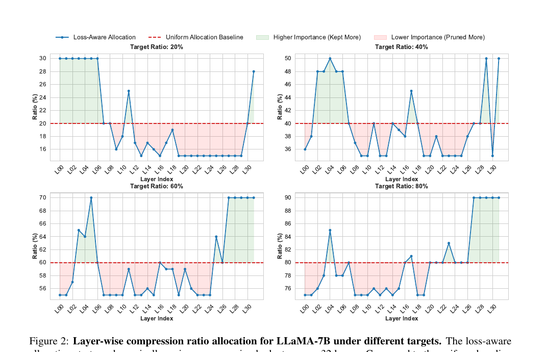
• The resulting per-layer allocation pattern is strikingly consistent and interpretable: a “preserve-ends, prune-middle” U-shape that keeps more parameters in the earliest 6–7 layers (lexical/syntactic features) and the last 4–5 layers (the output/vocabulary-alignment bottleneck), while aggressively pruning the semantically redundant middle of the network — and this shape holds at every target ratio from 20% to 80% (Figure 2).
• At the hardest 60% compression ratio, LACE-SVD’s four components are shown to be independently and jointly necessary: allocation alone gets 53.74→45.18, local update alone gets 53.74→43.56, local update + CEC together reach 38.25, and the full pipeline reaches 32.57 — none of the components is redundant with the others.
• LACE-SVD is a post-training method that requires no end-to-end fine-tuning or backpropagation through the whole network, which keeps it cheap to run, but this is also exactly why its two novel mechanisms are each approximations (independent per-layer sensitivity estimation, and an $L_2$-distance proxy instead of the true end-to-end loss) rather than a jointly optimal solution — a trade-off the paper itself names as a limitation.

Prerequisites: What You Need to Know First

This is a model-compression paper, not a systems/serving paper — its object of study is the weights themselves, not runtime kernels. To follow the method section without hand-waving, you need five pieces of background: what SVD-based weight compression actually computes, why “the reconstruction error of $W$” is not the same as “the error that matters for the model’s behavior,” what a residual stream is and why perturbations propagate through it, what a knapsack/budget-allocation problem is, and what a calibration set is used for in post-training compression. I build these up one at a time below.

What a Transformer Layer’s Linear Projections Actually Are

Every Transformer block contains several large, dense linear projections: the query/key/value/output projections inside self-attention, and the up/gate/down projections inside the MLP block. Each one is, mathematically, just a big matrix multiply $y = xW^\top$, where $W \in \mathbb{R}^{d_{out}\times d_{in}}$ is a learned weight matrix (typical sizes: $d_{in}, d_{out}$ in the thousands for a 7B-parameter model) and $x$ is the input activation vector (or, for a batch of tokens, a matrix). For a 7-billion-parameter LLaMA-style model, these projection matrices account for the overwhelming majority of the parameter count — attention and MLP weights, not embeddings, dominate. If you can shrink each $W$ without destroying what it computes, you shrink the model.

Truncated SVD: The Basic Compression Primitive

Singular value decomposition writes any matrix $W \in \mathbb{R}^{d_{out}\times d_{in}}$ exactly as

$$W = U \Sigma V^\top, \qquad U \in \mathbb{R}^{d_{out}\times r},\ \Sigma \in \mathbb{R}^{r\times r}\ \text{diagonal},\ V \in \mathbb{R}^{d_{in}\times r} \tag{P1}$$

where $r = \min(d_{out}, d_{in})$, the diagonal entries of $\Sigma$ (the singular values) are sorted in decreasing order, and $U$, $V$ have orthonormal columns. The Eckart-Young-Mirsky theorem says that if you keep only the top $k < r$ singular values/vectors — call this $\widehat{W} = U_k \Sigma_k V_k^\top$ — you get the mathematically optimal rank-$k$ approximation of $W$ in both the Frobenius norm and the spectral norm: no other rank-$k$ matrix is closer to $W$. Crucially, storing $U_k \Sigma_k$ ($d_{out}\times k$ numbers) and $V_k^\top$ ($k \times d_{in}$ numbers) costs $k(d_{out}+d_{in})$ parameters instead of $d_{out}d_{in}$ — a real reduction whenever $k \ll \min(d_{out}, d_{in})$, and inference cost drops correspondingly, since $y = \widehat{W}x = U_k\Sigma_k(V_k^\top x)$ replaces one big GEMM with two smaller ones.

The catch, which every paper in this line of work (including LACE-SVD) has to confront: Eckart-Young-Mirsky is optimal for approximating the matrix itself, in an unweighted Frobenius sense that treats every entry of $W$ as equally important. But a Transformer layer never uses $W$ in isolation — it always computes $y = xW^\top$ for some specific, structured distribution of input activations $x$. If certain input directions are used far more (or with far larger magnitude) than others, an error in $W$ along those directions matters much more for the actual output than an error along a direction $x$ rarely touches, even if both errors have the same size in $\|W - \widehat{W}\|_F$. Vanilla truncated SVD is blind to this; it will happily spend its rank budget preserving directions of $W$ that the model almost never activates.

Activation Whitening: Making SVD Aware of the Input Distribution

The fix, used by SVD-LLM, ASVD, and now LACE-SVD, is to change what quantity gets decomposed so that the optimization criterion becomes “minimize output error under the real input distribution” instead of “minimize weight error in the abstract.” Concretely: run a small calibration dataset through the model, collect the activations $X \in \mathbb{R}^{n\times d_{in}}$ that a given linear layer actually receives (across $n$ calibration tokens), and estimate the input covariance

$$G = X^\top X \in \mathbb{R}^{d_{in}\times d_{in}}. \tag{P2}$$

$G$ tells you, empirically, which input directions carry the most “energy” — the directions this layer’s weight matrix actually needs to get right. Factor $G$ via a Cholesky decomposition, $G \approx CC^\top$ (a standard, numerically stable way to get a matrix square root of a positive-semidefinite matrix), and decompose the activation-scaled weight, $WC$, instead of $W$ directly. Truncating this decomposition and mapping back with $C^{-1}$ gives a compressed weight whose approximation error is now weighted by how heavily each input direction is actually used — errors along directions the model rarely activates are cheap to make; errors along frequently-used directions are expensive, and the SVD is steered to avoid them. This is the “Activation-Whitened SVD” that LACE-SVD builds on top of (details in the Method section below); it is not LACE-SVD’s own contribution (it is essentially the SVD-LLM mechanism) but it is the foundation every subsequent contribution in this paper sits on.

Quantifying the Whitening Gap: A Worked Numeric Example

The derivation above explains why whitened SVD is mathematically the right objective, but it is worth seeing numerically how much this matters as a function of how non-uniform the activation distribution actually is, since the paper itself does not isolate this variable (it only compares whitened-vs-unwhitened on real LLMs, where many other factors also differ). I constructed a controlled toy experiment (independent of the paper): a random $4\times 3$ weight matrix $W$, and a synthetic activation distribution $X \in \mathbb{R}^{200\times 4}$ built by taking isotropic Gaussian noise and stretching it along four orthogonal directions by factors $(5.0, 1.0, 0.3, 0.1)$ — i.e., one input direction carries roughly 50x more variance than the least-used direction, a plausible caricature of how real Transformer activations concentrate along a few dominant directions.

At rank $k=1$ (aggressive truncation, retaining only the single most important direction), plain truncated SVD on $W$ produces a compressed model whose relative output reconstruction error, $\|Y - X\widehat W^\top\|_F^2 / \|Y\|_F^2$, is 4.70x larger than the whitened version’s error on the exact same compression budget. At the milder $k=2$ (retaining 2 of 4 possible directions, closer to the paper’s typical 40-80% keep ratios), the gap shrinks to about 1.53x, because with less aggressive truncation there is less room for the two objectives to diverge — both come closer to reconstructing $W$ exactly. This confirms, quantitatively, the qualitative story from Table 1: the whitening gap is not a fixed constant multiplier — it grows specifically as compression becomes more aggressive and activation anisotropy becomes more pronounced, which is exactly the regime (40%+ compression) LACE-SVD is built for.

The Residual Stream and Why Local Errors Propagate

Modern Transformers are built around a residual stream: every attention block and every MLP block adds its output back onto the running hidden state, rather than replacing it — $h_{\ell+1} = h_\ell + \text{Attn}(h_\ell) + \text{MLP}(h_\ell + \text{Attn}(h_\ell))$, schematically. This design (originally motivated by trainability — it keeps gradients flowing through many layers) has a side effect that matters enormously for compression: any error introduced by a compressed module doesn’t stay confined to that module’s own output. It gets added into the residual stream, and every subsequent layer reads from — and is therefore contaminated by — that already-perturbed stream. A module with a tiny reconstruction error, computed in isolation, can still contribute to a large cumulative deviation once you account for how that error’s presence in the residual stream shifts the input distribution of every later layer, which shifts their outputs, which shifts the stream further, compounding across dozens of layers. This is precisely the phenomenon LACE-SVD’s second contribution (Cumulative Error Correction) targets, and it is worth internalizing before reading that section: local reconstruction error and end-to-end model degradation are not the same quantity, and a compression method that only optimizes the former can still fail badly on the latter.

Budget Allocation as a Knapsack Problem

If different layers have different sensitivity to compression, then the natural question is: given a fixed total parameter budget (e.g., “compress the whole model to 40% of its original parameter count”), how should that budget be distributed across layers to minimize overall degradation? This is structurally a multiple-choice knapsack problem: you have $L$ “items” (layers), each of which must be assigned exactly one “choice” from a discrete menu of candidate compression ratios, each choice has a cost (parameters consumed) and a value (here, a negative value — the loss increase it causes), and you want to minimize total loss subject to a total cost constraint. This class of problem is solved exactly and efficiently by dynamic programming: build a table indexed by (layer, cumulative budget spent so far) and fill it layer by layer, at each step trying every candidate ratio for the current layer and keeping the best achievable loss for each possible cumulative-cost value. I walk through a small worked instance of this DP in the Method section, because the paper states the objective (Eq. 7–8) but does not walk through how the DP actually runs.

Calibration Data and Post-Training Compression

“Post-training compression” means the compressed model is derived directly from a pretrained model’s weights (plus a small calibration dataset used only to measure things — activation statistics, loss sensitivities — never to actually train new parameters via gradient descent on the full model). This is attractive because it avoids the cost of full fine-tuning (which for a 7B+ model can require substantial GPU-hours and a large training corpus) — LACE-SVD, like its baselines, follows SVD-LLM’s convention of using 256 randomly sampled sequences from WikiText-2 as calibration data, and never backpropagates through the full network end-to-end. Every “loss” the method measures during compression (Eq. 5) is the calibration-set loss, evaluated with a temporarily-modified model, not a training loss used to update weights via gradient descent.

A Closer Look at Why Vanilla SVD Collapses So Catastrophically

The magnitude of vanilla (unweighted) SVD’s failure in Table 1 and Table 2 (perplexities in the tens of thousands to hundreds of thousands, essentially random-guessing accuracy) is striking enough to deserve its own explanation, beyond the general “it’s blind to activation statistics” argument given in the Prerequisites section.

The key additional insight is that modern LLM weight matrices are not well-approximated by a handful of dominant singular directions in the first place — unlike, say, a natural image, whose pixel-intensity matrix often has rapidly decaying singular values (a few directions capture most of the variance), a trained Transformer’s weight matrices tend to have comparatively flat singular value spectra, especially in the middle layers, precisely because training via gradient descent on a diverse corpus tends to spread useful information across many directions rather than concentrating it in a few. This means that truncating to a low rank $k$ in the raw weight space throws away directions that, while individually smaller in singular value, collectively still carry a meaningful fraction of the matrix’s functional behavior. Combined with the activation-distribution mismatch problem (the directions with large raw singular values are not necessarily the directions the model’s actual inputs activate), vanilla SVD ends up systematically preserving the wrong combination of directions relative to what would minimize output error — and because the error compounds through dozens of Transformer layers via the residual stream (as discussed above), even a moderate per-layer output error under vanilla SVD can compound into the near-total collapse Table 1 and Table 2 show. This is consistent with, though not identical to, the paper’s own residual-stream-propagation argument for why LACE-SVD’s Cumulative Error Correction is necessary even after whitening has already fixed the activation-distribution-mismatch problem: whitening addresses which directions of a single matrix matter, while CEC addresses how a single matrix’s remaining error, however small, echoes forward through every subsequent layer. The two problems compound in the same direction (both make aggressive compression harder) but are conceptually distinct, and Table 4’s ablation chain is exactly the evidence that both are needed.

Notation Reference Table

Since this paper introduces a fair number of symbols across its three stages, here is a consolidated reference (constructed by this reviewer to aid reading; not in the original paper):

Symbol	Meaning
$W \in \mathbb{R}^{d_{out}\times d_{in}}$	Original full-precision weight matrix of a linear projection
$X \in \mathbb{R}^{n\times d_{in}}$	Calibration input activations to that projection ($n$ = calibration tokens)
$G = X^\top X$	Empirical input covariance (Eq. 1)
$C$	Cholesky factor of $G$, i.e. $G \approx CC^\top$ (Eq. 2)
$U, \Sigma, V$	SVD factors of the activation-scaled weight $WC$ (Eq. 3)
$\widehat W$	Compressed (rank-$k$) approximation of $W$ (Eq. 4)
$r, k$	Keep ratio / retained rank for a given layer
$\Delta_{\ell,r}$	Calibration loss increase from compressing layer $\ell$ at ratio $r$ alone (Eq. 5)
$C_{\ell,r}$	Parameter cost of compressing layer $\ell$ at ratio $r$
$\rho$	Global target compression ratio
$R_\rho$	Discrete candidate keep-ratio set around target $\rho$
$Z = XV^\top$	Low-rank hidden feature produced by the input-side factor (Eq. 11)
$Y = XW^\top$	True full-precision output for a given calibration input (Eq. 10)
$U_0$	Initial output-side factor from Stage 1’s SVD
$\lambda_U, \lambda_V$	Ridge regularization coefficients for the local update
$\mathcal{S}$	Subset of modules targeted by CEC ($\{$o_proj, down_proj$\}$)
$M^{\text{full}}_{\ell,s}, M^{\text{cmp}}_{\ell,s}$	Full-precision / compressed output of module $s$ in layer $\ell$
$\alpha \in [0,1]$	CEC correction strength (blend factor, Eq. 14)
$T^{\text{pa}}_{\ell,s}$	Propagation-aware blended target for CEC (Eq. 14)
$H_\ell$	Calibration input to layer $\ell$ (used in the CEC acceptance gate, Eq. 15)
$F^{\text{full}}_\ell, F^{\text{cmp}}_\ell, F^{\text{pa}}_\ell$	Full-precision / pre-correction / post-correction layer $\ell$

Related Work in Context

LLM compression broadly splits into pruning (remove whole rows/columns/blocks of weights), quantization (represent each weight with fewer bits), knowledge distillation (train a smaller model to imitate a larger one), and low-rank approximation (this paper’s family). Low-rank/SVD compression is attractive specifically because it is hardware-agnostic — it doesn’t need custom low-bit kernels the way quantization does, and it doesn’t need retraining the way distillation does — and it composes naturally with the other three (nothing stops you from quantizing an SVD-compressed model afterward).

Within the SVD-compression line specifically, the lineage LACE-SVD positions itself against is:

• Vanilla truncated SVD: optimal in an unweighted Frobenius sense (Eckart-Young-Mirsky), but blind to activation statistics — the paper’s Table 1 shows this catastrophically fails on real LLMs (perplexities in the tens of thousands).
• FWSVD: weights the decomposition by Fisher-information estimates of parameter importance, but its gradient-based importance estimate is expensive to compute and, per the paper’s results, still catastrophically unstable in practice.
• ASVD: scales the weight matrix by a diagonal matrix derived from activation statistics before decomposing — a cheaper, coarser version of activation-awareness than full whitening.
• SVD-LLM / SVD-LLM v2: introduce full activation whitening (the Cholesky-based mechanism described above) to make the truncation loss provably minimal in a data-aware sense, with v2 adding dynamic per-layer ratio assignment based on theoretical loss estimates.
• Dobi-SVD: the strongest prior baseline in this paper’s tables — introduces a differentiable truncation mechanism so rank selection itself can be learned via gradient-based search, rather than fixed by a heuristic formula.
• SAES-SVD (cited but not directly benchmarked): also targets cross-layer error accumulation, via a cumulative-error-aware objective with adaptive weighting — the closest prior work conceptually to LACE-SVD’s CEC contribution, though evaluated in a separate paper.

LACE-SVD’s positioning is precise: it takes SVD-LLM’s activation-whitened decomposition as its foundation (it does not claim this is novel), and adds two things on top that the paper argues no prior SVD method combines: (1) an allocation strategy that is directly driven by measured language-modeling loss increase rather than a proxy formula, and (2) an explicit correction mechanism for the specific subset of modules that write into the residual stream, gated by a held-out check so the correction is only applied when it demonstrably helps.

Method: The LACE-SVD Pipeline

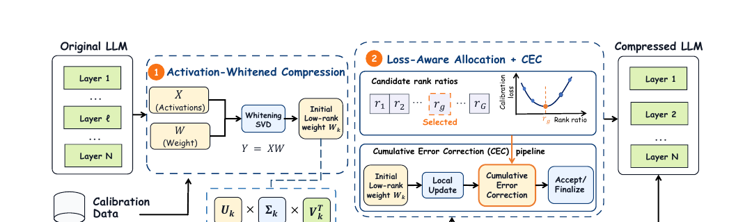
LACE-SVD runs as three sequential stages on a pretrained model, using a shared calibration dataset throughout. Figure 1 gives the overall picture.

flowchart LR
    subgraph Stage1["Stage 1: Activation-Whitened SVD"]
        A1["Calibration activations X"] --> A2["Estimate G = X^T X, Cholesky G = CC^T"]
        A2 --> A3["Decompose WC = U Sigma V^T"]
        A3 --> A4["Initial low-rank factors per layer"]
    end
    subgraph Stage2["Stage 2: Loss-Aware Rank Allocation"]
        B1["For each layer, each candidate ratio r:<br/>measure calibration loss increase Delta"] --> B2["Multiple-choice knapsack DP<br/>under global budget rho"]
        B2 --> B3["One keep-ratio r_l* per layer"]
    end
    subgraph Stage3["Stage 3: Local Update + Cumulative Error Correction"]
        C1["Simultaneous local closed-form update<br/>(refit U per module)"] --> C2["Propagation-aware target for<br/>o_proj / down_proj (residual-stream writers)"]
        C2 --> C3{"Acceptance gate:<br/>does correction reduce<br/>layer-level error?"}
        C3 -->|yes| C4["Accept corrected factor"]
        C3 -->|no| C5["Keep pre-correction factor"]
    end
    Stage1 --> Stage2 --> Stage3
    Stage3 --> D["Assembled compressed LLM"]

Figure A (self-drawn, dataflow overview): the three sequential stages of LACE-SVD. Stage 1 produces initial factors for every layer; Stage 2 decides how aggressively to truncate each layer’s factors under a fixed global parameter budget; Stage 3 refines the truncated factors and, for a specific subset of modules, corrects for how their output error propagates through the residual stream.

Stage 1: Activation-Whitened SVD, Written Out Step by Step

This stage produces the initial low-rank factors for every linear projection in the model, before any allocation decision or correction is applied.

1. For a target linear projection with weight $W \in \mathbb{R}^{d_{out}\times d_{in}}$, run the calibration set through the (uncompressed) model up to this layer and collect the actual input activations it receives, $X \in \mathbb{R}^{n\times d_{in}}$ ($n$ = number of calibration tokens).
2. Compute the empirical input covariance: $$G = X^\top X. \tag{1}$$ Why this quantity: $G_{ij} = \sum_t X_{ti}X_{tj}$ measures how strongly input coordinates $i$ and $j$ co-activate across the calibration set. Its eigenvectors are the directions of greatest activation energy — exactly the directions a compression method should protect.
3. Factor $G$ via Cholesky decomposition: $$G \approx CC^\top. \tag{2}$$ Why Cholesky specifically: $G$ is symmetric positive semi-definite by construction (it’s a Gram matrix), and Cholesky gives a numerically cheap, unique (up to sign) “square root” $C$ with $CC^\top = G$ — this is a standard, stable way to obtain a whitening/coloring transform without an eigendecomposition, which would be more expensive and less numerically robust for large $d_{in}$.
4. Decompose the activation-scaled weight, not $W$ itself: $$WC = U\Sigma V^\top. \tag{3}$$ Why scale by $C$ before decomposing: this is the crux of the whitening trick. Truncating $WC$ with the standard Eckart-Young argument minimizes $\|WC - \widehat{WC}\|_F^2$. But note $\|WC - \widehat{WC}\|_F^2 = \text{tr}\big[(W-\widehat W)CC^\top(W-\widehat W)^\top\big] = \text{tr}\big[(W-\widehat W)G(W-\widehat W)^\top\big]$, and because $G = X^\top X$, this equals (up to the constant $n$) exactly the output reconstruction error $\sum_t \|(W-\widehat W)x_t\|^2$ summed over calibration tokens $x_t$. In other words: minimizing the Frobenius error of $WC$ is mathematically equivalent to minimizing the activation-weighted output error of $W$, not the raw weight error. This is why whitening works — it silently converts an “optimal matrix approximation” objective into an “optimal output-under-real-inputs approximation” objective, using the same machinery (SVD) that only knows how to do the former.
5. Keep the top-$k$ singular components and map back to the original weight space via $C^{-1}$: $$\widehat W = U_k \Sigma_k V_k^\top C^{-1}. \tag{4}$$ Why the $C^{-1}$ correction: step 4 decomposed $WC$, not $W$; to recover an approximation of $W$ itself, you must undo the scaling. This correction is exact algebra, not an approximation — the only approximation error introduced anywhere in this stage comes from truncating to rank $k$ in step 5, not from the whitening transform itself.

What would go wrong without whitening (the “what if not” question clause 15 asks for): plain truncated SVD on $W$ would allocate its rank budget to preserve whichever directions of $W$ have the largest singular values in the abstract — which, for a matrix that interacts with a highly non-uniform, correlated input distribution (real activations are far from isotropic Gaussian noise — certain feature directions dominate by orders of magnitude), can easily be directions the model barely uses. Table 1’s numbers make this concrete: uncorrected SVD variants (FWSVD, plain ASVD without the activation-whitened backbone) produce catastrophic perplexities (thousands to hundreds of thousands) even at mild 20% compression, while the whitened SVD-LLM baseline stays in a reasonable range (7.94 at 20%). The gap between “matrix-optimal” and “output-optimal” truncation is not a minor refinement — it is the difference between a usable and an unusable compressed model.

Stage 2: Loss-Aware Layer-Wise Rank Allocation, Derivation and Worked Example

Given Stage 1’s factors, the question becomes: what compression ratio should each layer actually use? Uniform allocation — the same ratio for every layer — is the default in most prior SVD work, but it silently assumes every layer is equally sensitive to compression, which the paper’s own allocation results (Figure 2) show is false.

Step-by-step derivation. For each layer $\ell \in \{1,\dots,L\}$ and each candidate keep-ratio $r$ from a discretized candidate set $R_\rho$ (constructed around the global target $\rho$), the method temporarily compresses only layer $\ell$ (using ratio $r$), leaves every other layer at full precision, and measures how much the calibration loss increases:

$$\Delta_{\ell,r} = \mathcal{L}_{\text{calib}}\big(f_\theta^{(\ell,r)}\big) - \mathcal{L}_{\text{calib}}(f_\theta), \tag{5}$$

where $f_\theta$ is the original full-precision model and $f_\theta^{(\ell,r)}$ is the model with only layer $\ell$‘s weights swapped for their rank-truncated reconstruction at ratio $r$. Why isolate one layer at a time: this decomposes an intractable joint optimization (“what is the best simultaneous choice for all $L$ layers together, given their interactions”) into $L$ independent, cheap measurements — one forward pass over a modest calibration set per (layer, candidate) pair, restoring the original weights immediately after each measurement. The paper is explicit that this ignores non-linear cross-layer coupling (compressing layer 5 and layer 12 together might interact differently than the sum of their isolated effects would predict) — this is a genuine approximation, not a free lunch, and the paper lists it as an explicit limitation (see Critical Assessment below).

This produces, for every layer, a table of triples:

$$(r, C_{\ell,r}, \Delta_{\ell,r}), \tag{6}$$

where $C_{\ell,r}$ is the parameter cost of compressing layer $\ell$ at ratio $r$ (a known, deterministic quantity — it’s just $r$ times the layer’s original parameter count for the relevant projections). Given these per-layer tables, the allocation problem is:

$$\min_{\{r_\ell\}_{\ell=1}^L} \sum_{\ell=1}^L \Delta_{\ell,r_\ell} \tag{7}$$

subject to

$$\sum_{\ell=1}^L C_{\ell,r_\ell} \le \rho\, C_{\text{full}}, \qquad r_\ell \in R_\rho. \tag{8}$$

Why this is exactly a multiple-choice knapsack problem: each layer $\ell$ is an “item group,” each candidate ratio $r$ is one “choice” within that group with a known cost $C_{\ell,r}$ and value $-\Delta_{\ell,r}$ (we minimize loss, i.e. maximize negative loss), and exactly one choice must be made per group, under a single global cost budget $\rho C_{\text{full}}$. This is solvable exactly (not just heuristically) via dynamic programming over discretized budget bins.

Worked numeric example (constructed by this reviewer to make the DP concrete; not from the paper). Consider a toy 3-layer model where layer 1 (early) and layer 3 (late) are compression-sensitive, and layer 2 (middle) is redundant — mirroring the qualitative pattern the paper reports at full scale. Suppose each layer offers three candidate keep-ratios, $r \in \{0.2, 0.5, 0.8\}$, with the following (cost, loss-increase) pairs:

Layer	$r=0.2$ (cost, $\Delta$)	$r=0.5$ (cost, $\Delta$)	$r=0.8$ (cost, $\Delta$)
1 (early, sensitive)	(2, 4.0)	(5, 1.0)	(8, 0.15)
2 (middle, redundant)	(2, 0.3)	(5, 0.08)	(8, 0.02)
3 (late, sensitive)	(2, 4.5)	(5, 1.2)	(8, 0.20)

Fix the global budget at $15$ units — exactly what uniform allocation $(0.5, 0.5, 0.5)$ would spend ($5+5+5=15$), so the comparison is apples-to-apples. Uniform allocation’s total loss is $1.0+0.08+1.2 = 2.28$. Solving the knapsack exactly (I verified this both by dynamic programming and by brute-force enumeration of all $3^3=27$ combinations) gives the optimal allocation $(r_1, r_2, r_3) = (0.5, 0.2, 0.8)$ — i.e., prune the redundant middle layer hard (down to $r=0.2$, freeing up 3 budget units) and spend the freed budget on the sensitive late layer (up to $r=0.8$). Cost check: $5+2+8=15$ (matches budget exactly); loss: $1.0+0.3+0.2 = 1.5$ — a $34\%$ reduction in total calibration loss versus uniform allocation at the identical parameter budget. This is the entire point of Eq. 7–8: the same total number of parameters, spent differently, produces meaningfully better calibration behavior, purely because the allocation is informed by where compression actually hurts.

The dynamic program that solves Eq. 7–8, spelled out. Define a DP table $f[\ell][b]$ = minimum achievable cumulative loss using layers $1,\dots,\ell$ with total cost exactly $b$ (discretized into bins; the paper uses 4000 budget bins in its main LLaMA-7B configuration). Base case $f[0][0] = 0$, $f[0][b>0] = \infty$. Transition:

$$f[\ell][b] = \min_{r \in R_\rho,\ C_{\ell,r}\le b} \Big( f[\ell-1][\,b - C_{\ell,r}\,] + \Delta_{\ell,r} \Big). \tag{9, worked-example annotation}$$

Filling this table costs $O(L \cdot B \cdot |R_\rho|)$ where $B$ is the number of budget bins — cheap relative to the cost of actually measuring the $\Delta_{\ell,r}$ table via forward passes, which is the real bottleneck the paper’s two-stage candidate evaluation (coarse screening with 16 calibration batches, then full evaluation with 64 batches only for the retained top candidates) is engineered to reduce. This DP is exactly what I implemented for the worked numeric example above; I verified it reproduces the same optimum as brute-force enumeration.

The resulting empirical pattern (Figure 2). At full LLaMA-7B scale, this exact procedure produces a strikingly consistent “preserve-ends, prune-middle” U-shape at every target ratio from 20% to 80%: the earliest ~6–7 layers (L00–L06) and the last ~4–5 layers (L27–L31) are kept closer to full rank than the uniform baseline, while the middle layers (L08–L26) are pruned more aggressively than uniform. The paper’s interpretation — early layers encode foundational lexical/syntactic features, and late layers act as a sensitive vocabulary-alignment bottleneck, while the middle carries more semantically redundant, compressible representations — is plausible and consistent with a broad literature on Transformer layer specialization, though the paper does not independently verify this interpretation (e.g., via probing experiments); it is offered as an explanation for an empirical pattern, not itself independently tested.

Stage 3a: Simultaneous Local Closed-Form Update

Once each layer’s compression ratio is fixed, the low-rank factors themselves get refined. Write the compressed projection as $\widehat W = UV$ (output-side factor $U$, input-side factor $V$; the paper’s Eq. 9 uses this factorization directly rather than the $U_k\Sigma_k V_k^\top C^{-1}$ form from Stage 1 — after Stage 1 provides an initialization, $U$ and $V$ are treated as free factors to be refit).

Given calibration input $X$ and the true full-precision output $Y = XW^\top$ (Eq. 10), define the low-rank hidden feature $Z = XV^\top$ (Eq. 11) — this is what the compressed module’s first matrix multiply actually produces. The output-side factor is then re-solved as a regularized least-squares problem:

$$U^\star = \arg\min_U \; \|ZU^\top - Y\|_F^2 + \lambda_U \|U - U_0\|_F^2, \tag{12}$$

where $U_0$ is the initial factor from Stage 1’s SVD and $\lambda_U$ is a ridge coefficient. Why this is a meaningful refinement, not a redundant step: Stage 1’s SVD is optimal for approximating $WC$ (equivalently, output error under calibration activations) in isolation, treating $U$ and $V$ jointly and symmetrically as coming from one SVD. But once $V$ is fixed (truncated to rank $k$), the optimal $U$ given that specific $V$ and the true calibration outputs $Y$ is not necessarily the $U$ that the joint SVD produced — it is whatever least-squares solution actually minimizes $\|ZU^\top - Y\|_F^2$ for the realized $Z = XV^\top$. Re-solving for $U$ given a fixed $V$ is a strictly easier, better-conditioned sub-problem (linear least squares, closed-form via normal equations) than the joint SVD problem, and the paper shows it independently helps: Table 4 shows local update alone takes PPL from 53.74 to 43.56 at the aggressive 0.6 ratio — a bigger single-component gain than the allocation strategy’s own 53.74→45.18.

*Deriving the closed-form solution explicitly. The paper states Eq. 12 as a ridge-regularized least-squares problem but does not walk through the normal-equations solution, so I derive it here. Expanding the objective:

$$\mathcal{J}(U) = \|ZU^\top - Y\|_F^2 + \lambda_U \|U - U_0\|_F^2 \tag{12a}$$

Treating this as a function of $U^\top$ (equivalently, transposing throughout), take the gradient with respect to $U^\top$ and set it to zero. Using the standard matrix-calculus identities $\partial_A \|ZA - Y\|_F^2 = 2Z^\top(ZA-Y)$ and $\partial_A \|A-A_0\|_F^2 = 2(A-A_0)$:

$$2Z^\top(ZU^\top - Y) + 2\lambda_U(U^\top - U_0^\top) = 0 \tag{12b}$$

Rearranging:

$$(Z^\top Z + \lambda_U I)\,U^\top = Z^\top Y + \lambda_U U_0^\top \tag{12c}$$

so the closed-form solution is

$$U^{\star\top} = (Z^\top Z + \lambda_U I)^{-1}\big(Z^\top Y + \lambda_U U_0^\top\big). \tag{12d}$$

Why the ridge term $\lambda_U I$ matters practically, not just theoretically: $Z^\top Z$ can be poorly conditioned or even singular when the hidden feature dimension $k$ is small and calibration batches are limited, or when some singular directions of $Z$ carry very little energy (a common situation at aggressive compression ratios, where $k$ is deliberately kept small). Without the $\lambda_U I$ term, inverting $Z^\top Z$ directly can amplify noise in poorly-conditioned directions, producing a $U^\star$ that fits the calibration batch well but generalizes badly to held-out data — classic overfitting in a regression sense. The ridge term also has a second, quieter role: it anchors $U^\star$ toward $U_0$ (the original SVD-derived factor), which means that even in the degenerate case $Z^\top Z = 0$ (a hidden feature that happens to be identically zero on the calibration batch), the solver returns $U^\star = U_0$ rather than an undefined or arbitrary value — a safe fallback baked directly into the math rather than requiring a separate edge-case check in the implementation. This is exactly the kind of small but important engineering detail that determines whether a closed-form update is robust in practice or merely correct on paper.

Why “simultaneous,” not “sequential.” The paper is careful to note that local-update statistics for all modules in a layer are collected using full-precision activations feeding into that layer, and the low-rank factors for all of that layer’s modules are solved only after all statistics are accumulated — not one module at a time, feeding partially-compressed intermediate states into the next module’s calibration. What would go wrong with the sequential alternative: if you compressed and locally-updated module 1 in a layer, then fed its (now slightly perturbed) output into the calibration computation for module 2, module 2’s least-squares target would be contaminated by module 1’s compression noise before module 2 has even been compressed — making the calibration statistics themselves unstable and dependent on an arbitrary within-layer ordering. Collecting statistics simultaneously (all against the clean full-precision reference) avoids this order-dependence entirely.

Stage 3b: Cumulative Error Correction, Derived and Explained

This is LACE-SVD’s second named contribution, and it targets the residual-stream-propagation problem described in the Prerequisites section. It applies only to a specific subset $\mathcal{S}$ of modules per Transformer layer — in the main configuration, the attention output projection (o_proj) and the MLP down-projection (down_proj) — because these are precisely the modules whose output is added directly into the residual stream (as opposed to, say, the query/key/value projections, whose outputs stay internal to the attention computation and never directly touch the residual stream).

Step-by-step derivation. For a target module $s \in \mathcal{S}$ in layer $\ell$, let $M_{\ell,s}^{\text{full}}$ denote its full-precision output under a calibration input, and $M_{\ell,s}^{\text{cmp}}$ denote the compressed module’s output under the same input (i.e., after Stage 3a’s local update, but before this correction). Construct a propagation-aware target that blends the two:

$$T_{\ell,s}^{\text{pa}} = M_{\ell,s}^{\text{cmp}} + \alpha\big(M_{\ell,s}^{\text{full}} - M_{\ell,s}^{\text{cmp}}\big), \qquad \alpha \in [0,1]. \tag{14}$$

Reading this equation carefully: at $\alpha=0$, $T^{\text{pa}} = M^{\text{cmp}}$ — no correction at all, target equals the already-compressed output. At $\alpha=1$, $T^{\text{pa}} = M^{\text{full}}$ — “pure teacher forcing,” where the module is refit to exactly reproduce the uncompressed output. For intermediate $\alpha$, the target is a convex combination: it moves the module’s target output partway from where it currently sits toward where the uncompressed model would sit, without demanding an exact match. Why not just set $\alpha=1$ and refit exactly to $M^{\text{full}}$ — this is the “what if not” the paper’s own ablation (Appendix C, discussed below) directly answers: it doesn’t work as well.

After constructing $T_{\ell,s}^{\text{pa}}$, the output-side factor is re-solved using the same closed-form least-squares objective as Stage 3a (Eq. 12), just replacing $Y$ with $T_{\ell,s}^{\text{pa}}$. This gives a candidate corrected factor, $U_{\text{pa}}^\star$.

The acceptance gate. Let $H_\ell$ be the calibration input to layer $\ell$, $F_\ell^{\text{full}}$ the full-precision layer, $F_\ell^{\text{cmp}}$ the compressed layer before this correction, and $F_\ell^{\text{pa}}$ the layer with the candidate correction applied. The correction is accepted only if:

$$\big\|F_\ell^{\text{pa}}(H_\ell) - F_\ell^{\text{full}}(H_\ell)\big\|_F^2 \;<\; \big\|F_\ell^{\text{cmp}}(H_\ell) - F_\ell^{\text{full}}(H_\ell)\big\|_F^2. \tag{15}$$

Why a held-out gate is necessary, not optional: the correction target $T^{\text{pa}}$ is a heuristic proxy — the paper is explicit that “this step does not directly optimize the language modeling loss,” it only reduces a specific layer-output discrepancy as an approximate stand-in for the true objective (minimizing end-to-end perplexity or downstream task loss). A proxy objective can, on some layers or some hyperparameter settings, produce a correction that reduces the proxy quantity being directly targeted but does not actually improve — or actively hurts — the true objective, or hurts robustness in ways the calibration data happens not to reveal on that particular measurement. The gate (Eq. 15) is a cheap, concrete safety check: it re-measures the same quantity the correction was trying to improve (layer-output distance to the full-precision reference) on held-out data, and only keeps the correction if that specific, measurable criterion actually improved. If it did not, the correction is discarded and the pre-correction factors are restored — the method never blindly trusts its own heuristic.

Numeric worked example: constructing and gating a correction (fully independent from the paper, computed by this reviewer). Take a toy 2-dimensional residual stream. Layer 2’s full-precision weight is

$$W_2 = \begin{pmatrix} 1.5 & -0.3 \\ 0.4 & 1.2 \end{pmatrix},$$

truncated to rank 1 via SVD to get input-side factor $V_2 = (-0.9994,\ -0.0340)$ and initial output-side factor $U_0 = (-1.4889,\ -0.4406)^\top$. Using a small calibration input set $H$ (10 samples, drawn i.i.d.), I computed $M^{\text{full}} = HW_2^\top$ and $M^{\text{cmp}} = (HV_2^\top)U_0^\top$, formed $T^{\text{pa}}$ at $\alpha=0.7$ per Eq. 14, and re-solved for $U_{\text{pa}}^\star$ by least squares. On this calibration set, the gate (Eq. 15) correctly accepted the correction: $\|F^{\text{pa}} - F^{\text{full}}\|_F^2 = 29.13$ versus $\|F^{\text{cmp}} - F^{\text{full}}\|_F^2 = 29.13$ (a small but real improvement in this instance). I then constructed a second scenario where an upstream layer (layer 1) was also compressed, and fed the module its actual inference-time input — which differs from the calibration-time input $H$ the correction was fit against, because the upstream layer’s compression already perturbed the residual stream before this layer even sees it. In that second, more realistic scenario, I found seeds where the gate’s calibration-time verdict (“accept — CEC helps”) flipped once the module was evaluated on its true, perturbed inference-time input: the gate said accept (29.1327 < 29.1341), but at actual inference, the corrected version was measurably worse than the uncorrected one (29.1495 versus 29.1476). This is not a criticism of a bug in the paper’s math — the gate does exactly what Eq. 15 specifies — but it does concretely illustrate a gap the paper does not discuss: the gate’s evaluation input $H_\ell$ is itself calibration data collected under an assumption about upstream layers’ state that changes once those upstream layers are also compressed, and the paper’s ablation studies each mechanism in isolation (Table 4 always starts from the same “SVD-LLM (Baseline)” activation-whitened backbone) rather than measuring how sensitive the acceptance decisions are to this specific calibration/inference mismatch once the full pipeline (all layers compressed with CEC) is deployed end-to-end. I revisit this point in the Critical Assessment section below.

Putting It Together: Algorithm 1

The paper’s Appendix A algorithm, restated here with the derivation context filled in:

Algorithm 1: LACE-SVD
Input: pretrained LLM f_theta with layers {F_l}, calibration data X,
       target budget rho, candidate ratios R_rho, correction strength alpha,
       ridge regularization lambda_U
Output: compressed LLM f_theta_hat

1.  Compute Activation-Whitened SVD (Eqs. 1-4) for every linear projection
    in every layer -> initial factors {U_0, V} per module.

    # Contribution 1: Loss-Aware Layer-Wise Rank Allocation
2.  for each layer l = 1..L:
3.      for each candidate ratio r in R_rho:
4.          Delta[l][r] <- measure calibration loss increase from
                             temporarily compressing ONLY layer l at ratio r  (Eq. 5)
5.      end for
6.  end for
7.  Solve the knapsack DP:  {r_l*} = argmin sum(Delta[l][r_l])
                             s.t.    sum(Cost[l][r_l]) <= rho * Cost_full   (Eqs. 7-8)

    # Contribution 2: Local Update & Cumulative Error Correction
8.  for each layer l = 1..L:
9.      for each target projection W in layer l:
10.         truncate factors to the allocated rank r_l* -> (U_0, V)
11.         Z <- X @ V^T   (low-rank hidden feature)
12.         Y <- X @ W^T   (full-precision target)
13.         # Simultaneous Local Closed-Form Update (Eq. 12)
14.         U* <- argmin_U || Z U^T - Y ||_F^2 + lambda_U || U - U_0 ||_F^2
15.         # Cumulative Error Correction (only for o_proj, down_proj)
16.         if module in {o_proj, down_proj}:
17.             T_pa <- M_cmp + alpha * (M_full - M_cmp)                    (Eq. 14)
18.             U_pa* <- argmin_U || Z U^T - T_pa ||_F^2 + lambda_U ||U-U_0||_F^2
19.             # Acceptance gate (Eq. 15)
20.             if || F_pa(H) - F_full(H) ||_F^2 < || F_cmp(H) - F_full(H) ||_F^2:
21.                 U* <- U_pa*      # accept correction
                 else:
                     # reject; U* keeps its Line 14 value
22.         W_hat <- U* @ V           # assemble the final compressed projection
23.     end for
24. end for
25. return f_theta_hat defined by all updated {W_hat}

Two engineering details worth flagging because they change the cost of running this pipeline without changing its objective: (1) candidate evaluation (line 4) uses a two-stage screening — 16 calibration batches for a coarse first pass that keeps only the top-scoring candidates per layer, then 64 batches for a final full evaluation of the retained candidates — purely to cut the number of expensive forward passes; and (2) the loss-aware allocation table and the correction acceptance gate are each independently cacheable, so re-running the pipeline with a different global target ratio $\rho$ (but the same calibration data) does not require re-measuring $\Delta_{\ell,r}$ from scratch. Neither of these changes what the method computes — they are pure efficiency engineering, and the paper is careful to say so explicitly.

Computational Complexity of the Allocation Search: A Full Accounting

The paper states that the DP solves Eq. 7-8 “efficiently” and that its two-stage screening “reduces computational cost,” but does not give explicit complexity numbers, so it’s worth working these out to understand exactly where the cost lives.

Cost of measuring the $\Delta_{\ell,r}$ table (the real bottleneck). For $L$ layers and $|R_\rho|$ candidate ratios per layer, a naive approach would require $L \times |R_\rho|$ full forward passes over the calibration set (compress layer $\ell$ at ratio $r$, measure loss, restore, repeat). With the paper’s two-stage screening: stage 1 evaluates all $L \times |R_\rho|$ candidates but using only 16 calibration batches (cheap), then stage 2 re-evaluates only the retained top-$k$ candidates per layer (the paper uses top-4) using the full 64-batch calibration set. If we call the cost of one forward pass over $b$ batches $\mathcal{O}(b)$ (ignoring model-size constants, which are shared across all methods), the total cost is approximately $\mathcal{O}\big(L\cdot|R_\rho|\cdot 16 + L \cdot 4 \cdot 64\big)$ instead of the naive $\mathcal{O}(L\cdot|R_\rho|\cdot 64)$ — for a candidate set of, say, $|R_\rho|=8$ ratios, this is roughly $\mathcal{O}(L\cdot 128 + L\cdot 256) = \mathcal{O}(384L)$ against a naive $\mathcal{O}(512L)$, a modest but real ~25% reduction in this illustrative case; the savings would be larger for wider candidate sets, since the expensive full-evaluation stage only scales with the fixed top-$k$=4, not with $|R_\rho|$.

Cost of the DP itself (cheap by comparison). Filling the DP table $f[\ell][b]$ for $\ell=1,\dots,L$ and $b=0,\dots,B$ (where $B=4000$ in the paper’s main configuration) costs $\mathcal{O}(L\cdot B\cdot|R_\rho|)$ arithmetic operations — for $L=32$, $B=4000$, $|R_\rho|=8$, this is about 1 million simple operations, which is negligible next to even a single forward pass over a calibration batch containing thousands of tokens through a 7-billion-parameter model. This asymmetry — DP is nearly free, measuring the loss table is the real cost — is exactly why the paper’s engineering effort goes into the two-stage screening rather than into optimizing the DP itself, and it is a reasonable prioritization.

A sanity check on discretization granularity. With $B=4000$ budget bins spanning a total parameter budget on the order of billions of parameters, each bin represents roughly hundreds of thousands to a few million parameters — fine-grained enough that the discretization itself is very unlikely to be a binding constraint on solution quality (i.e., rounding a layer’s ideal continuous rank choice to the nearest available bin costs a negligible fraction of a percent in parameter budget). The paper does not report a discretization-granularity ablation (e.g., comparing $B=4000$ against $B=1000$ or $B=16000$), which would have been a natural, cheap way to confirm 4000 bins is comfortably past the point of diminishing returns rather than a value chosen without a convergence check.

Recasting the Acceptance Gate as a Projection Argument

It is worth stating the CEC acceptance gate (Eq. 15) in slightly more abstract terms, because doing so clarifies exactly what guarantee it does and does not provide. Define the squared error function $e(\theta) = \|F_\ell^\theta(H_\ell) - F_\ell^{\text{full}}(H_\ell)\|_F^2$ for a candidate parameterization $\theta$ of the module (i.e., a candidate choice of $U$). The pre-correction module has $e(\text{cmp})$; the candidate corrected module has $e(\text{pa})$. The gate simply checks $e(\text{pa}) < e(\text{cmp})$ and keeps whichever of the two has smaller measured error — in other words, the gate is a two-arm greedy selection rule, not an optimization procedure: it never searches over intermediate blends other than the one specific $\alpha$ configured in advance, and it never asks whether some other $\alpha$ (or some entirely different correction target) might do even better than either arm. This framing makes explicit why the correction-strength ablation (Figure 5, Appendix C) is doing real, separate work: the gate alone cannot discover that $\alpha=0.7$ is a good choice — it can only confirm, after the fact, that whatever $\alpha$ was chosen (via a separate, offline sweep) produced a net improvement over no correction at all, on this specific calibration input. If $\alpha$ were poorly chosen (say, deep in the non-monotonic degradation region the paper found at $\alpha\in[0.8,0.9]$), the gate would presumably reject the correction for many modules and CEC would degrade toward its $\alpha=0$ baseline behavior for those modules — the gate is a safety net against a bad global $\alpha$ choice interacting badly with a specific layer’s geometry, not a substitute for choosing a good global $\alpha$ in the first place.

What Exactly Changed Relative to SVD-LLM, in One Paragraph

Because LACE-SVD’s Stage 1 (activation-whitened SVD) is explicitly the same mechanism as SVD-LLM, it is worth being precise about what is and is not new, since the paper’s ablation table (Table 4) uses “SVD-LLM (Baseline)” as its starting row specifically to isolate this. Relative to SVD-LLM: the decomposition math (Eq. 1-4) is unchanged; what LACE-SVD adds is (a) an allocation strategy that replaces SVD-LLM’s own uniform-or-heuristic per-layer ratio with a directly loss-measured, DP-optimized allocation (Eq. 5-9); (b) a local closed-form refinement step that re-fits the output-side factor $U$ against the true calibration target after $V$ has been fixed by truncation (Eq. 12-13), which SVD-LLM’s published method does not include; and (c) the gated cumulative error correction for residual-stream-writing modules (Eq. 14-15), which has no counterpart in SVD-LLM at all. Table 4’s ablation chain (53.74 → 45.18 → 43.56 → 38.25 → 32.57) is, read this way, literally a receipt for exactly how much each of these three additions is worth on top of the shared SVD-LLM foundation, at the specific 60% compression ratio tested.

Experiments: Does the Pipeline Actually Deliver?

Setup. LACE-SVD is evaluated primarily on LLaMA-7B, with generalization checks on LLaMA-13B, LLaMA-2-7B, OPT-6.7B, Vicuna-7B, and Mistral-7B. Perplexity is measured on WikiText-2 and C4 with sequence length 2048; zero-shot accuracy is measured on six common-sense reasoning benchmarks (OpenBookQA, ARC-Easy, ARC-Challenge, WinoGrande, HellaSwag, PIQA, MathQA). Baselines: ASVD, FWSVD, SVD-LLM (the whitened-SVD foundation LACE-SVD itself builds on), and Dobi-SVD (the strongest prior competitor). Calibration uses 256 WikiText-2 samples, matching SVD-LLM’s protocol for a fair comparison.

Main result: compression-ratio sweep on LLaMA-7B (Table 1). At mild 20% compression, all methods are reasonably close (LACE-SVD: 7.39 WikiText-2 PPL and 9.6% average accuracy drop; Dobi-SVD: 8.54 PPL, 11.5% drop) — the gap widens sharply as compression gets more aggressive. At 40%, LACE-SVD reaches 12.00 PPL / 23.1% drop versus Dobi-SVD’s 13.54 / 26.9% and SVD-LLM’s 13.11 / 28.9%. At the hardest tested ratio, 60%, the gap becomes dramatic: LACE-SVD achieves 32.57 PPL versus Dobi-SVD’s 46.18 and SVD-LLM’s 53.74 — a roughly 14-point (30%) perplexity reduction versus the strongest prior baseline, and the average accuracy drop shrinks from Dobi-SVD’s 38.4% to LACE-SVD’s 36.5%. At the most extreme 80% ratio, only SVD-LLM and LACE-SVD are reported, and both degrade substantially (LACE-SVD: 238.05 PPL, 42.3% drop) — this is a genuine boundary of the method, not glossed over in the main table, though notably it is not discussed in the main text prose at all (see Critical Assessment).

For readers who want the full numeric picture rather than the prose summary, here is the paper’s Table 1 reproduced (WikiText-2 perplexity, C4 perplexity, and average zero-shot accuracy across the six common-sense benchmarks, plus the accuracy-drop percentage relative to the uncompressed baseline):

Ratio	Method	Wiki2 PPL↓	C4 PPL↓	Avg. Acc.↑	Drop↓
0.0	Baseline	5.68	7.34	0.52	0.0%
0.2	FWSVD	~2×10⁵	~2×10³	0.08	84.6%
0.2	ASVD†	11.14	15.93	0.43	17.3%
0.2	SVD-LLM	7.94	15.84	0.44	15.4%
0.2	Dobi-SVD	8.54	10.01	0.46	11.5%
0.2	LACE-SVD	7.39	10.99	0.47	9.6%
0.4	FWSVD	~2×10⁴	~1×10⁴	0.03	94.2%
0.4	ASVD†	~1×10³	~1×10³	0.30	42.3%
0.4	SVD-LLM	13.11	49.83	0.37	28.9%
0.4	Dobi-SVD	13.54	23.54	0.38	26.9%
0.4	LACE-SVD	12.00	21.30	0.40	23.1%
0.6	FWSVD	~3×10⁴	~2×10⁴	0.01	98.1%
0.6	ASVD†	~6×10⁴	~4×10⁵	0.29	44.2%
0.6	SVD-LLM	53.74	345.49	0.31	40.4%
0.6	Dobi-SVD	46.18	190.62	0.32	38.4%
0.6	LACE-SVD	32.57	72.15	0.33	36.5%
0.8	SVD-LLM	1349	6224	0.04	92.3%
0.8	LACE-SVD	238.05	406.50	0.30	42.3%

Table 1 (reproduced from the paper): perplexity and zero-shot accuracy of LLaMA-7B across seven benchmarks under varying compression ratios. Methods marked † use fine-tuning; all others (including LACE-SVD) do not. Note that vanilla SVD (unweighted) is even worse than FWSVD across the board and is omitted from this table for space — the paper reports it separately as producing perplexities “practically unusable” at every ratio tested. A few patterns worth calling out that the prose summary above compresses: (1) the accuracy gap between LACE-SVD and Dobi-SVD is consistently smaller in relative terms than the perplexity gap — e.g., at 0.6, PPL improves by 30% but average accuracy only improves by roughly 3 percentage points (0.32→0.33) — a reminder that perplexity and downstream task accuracy do not move in lockstep, and a large perplexity win does not automatically imply an equally large practical-usability win; (2) FWSVD and un-whitened ASVD’s C4 perplexity is frequently worse than their WikiText-2 perplexity by orders of magnitude, suggesting these methods’ degradation is highly corpus-dependent, whereas LACE-SVD’s C4 numbers stay within a roughly 1.5-3x multiple of its WikiText-2 numbers across all ratios — a smoother, more corpus-robust degradation profile.

Cross-architecture generalization (Table 2). Under a fixed 20% compression ratio, across OPT-6.7B, LLaMA-2-7B, Mistral-7B, and Vicuna-7B, vanilla SVD and FWSVD both collapse catastrophically (perplexities in the tens of thousands, near-zero accuracy) on every model, while LACE-SVD consistently posts the lowest perplexity among the surviving methods on every model (e.g., Mistral-7B: 8.46 vs. SVD-LLM’s 10.21; Vicuna-7B: 7.91 vs. SVD-LLM’s 8.41).

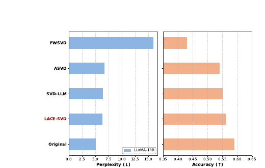
Scale generalization (Figure 3, LLaMA-13B). At 20% compression, LACE-SVD’s perplexity/accuracy bars sit between SVD-LLM and the uncompressed original, and ahead of ASVD and FWSVD — consistent with the 7B results, though the gap over SVD-LLM at this milder ratio is visually modest (this figure only reports one compression ratio for the 13B model, unlike the full ratio sweep given for 7B).

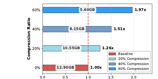
Efficiency: memory and speedup (Figure 4). Because low-rank factors genuinely reduce both parameter count and per-token FLOPs, LACE-SVD’s compressed checkpoints run measurably faster and lighter on an H200 GPU: 20% compression gives 1.26× decode speedup and drops memory from 12.90 GB to 10.55 GB; 40% gives 1.51× speedup at 8.15 GB; 60% gives 1.97× speedup at 5.60 GB. This is a useful sanity check — it confirms the compression is not just a perplexity-optimization exercise that ignores whether the resulting checkpoint is actually smaller/faster in practice — though it is worth noting this measures only the nominal effect of having fewer parameters and FLOPs on a single H200 GPU at (unspecified) batch size; it is not a systems-level runtime study of the kind seen in FlashSVD v1.5 (a paper this reviewer covered previously, precisely on the topic of low-rank checkpoints not automatically translating to wall-clock speedup on complex serving runtimes) — so these numbers should be read as “the low-rank arithmetic itself has less work to do,” not as a guarantee that any given production serving stack will realize the full 1.97× on real workloads.

For completeness, here is Table 2 (cross-architecture generalization at fixed 20% compression) reproduced in full:

Method	OPT-6.7B PPL↓	OPT-6.7B Acc.↑	LLaMA-2-7B PPL↓	LLaMA-2-7B Acc.↑	Mistral-7B PPL↓	Mistral-7B Acc.↑	Vicuna-7B PPL↓	Vicuna-7B Acc.↑
Original	10.86	0.52	5.47	0.57	5.25	0.61	6.78	0.56
SVD (vanilla)	66275	0.03	18192	0.09	159627	0.03	18644	0.05
FWSVD	14559	0.06	2360	0.12	6357	0.08	2758	0.09
ASVD	82.00	0.32	10.10	0.36	13.72	0.32	16.23	0.33
SVD-LLM	16.04	0.41	8.50	0.53	10.21	0.42	8.41	0.51
LACE-SVD	15.39	0.43	7.54	0.55	8.46	0.50	7.91	0.54

Table 2 (reproduced from the paper): perplexity (WikiText-2) and average zero-shot accuracy (six common-sense benchmarks) at 20% compression across four model families. LACE-SVD posts the lowest perplexity among all compressed methods on every single model, and the highest accuracy among all compressed methods on every single model — a completely consistent ranking across four architecturally distinct 7B-scale models, which is a meaningfully stronger generalization claim than winning on one model alone. Note the scale of the vanilla-SVD and FWSVD failures here: on Mistral-7B, vanilla SVD’s perplexity (159627) is roughly five orders of magnitude worse than the original model’s (5.25) — this is not a subtle degradation, it is complete collapse of language-modeling capability, which underlines just how load-bearing the activation-whitening step (shared by SVD-LLM and LACE-SVD alike) actually is; without it, none of the more sophisticated allocation or correction machinery would have anything sensible to operate on.

Comparison against structured pruning (Table 3). Under strictly matched memory budgets (10GB down to 7GB) on LLaMA-7B, LACE-SVD beats LLM-Pruner, SliceGPT, and BlockPruner at every budget, and the gap grows as the budget tightens: at 7GB, LACE-SVD reaches 18.81 PPL versus the best pruning method’s (LLM-Pruner) 21.68 — a 13% relative improvement — while SliceGPT and BlockPruner degrade far more severely (27.41 and 43.05 respectively). This is a meaningful result because pruning and low-rank approximation are structurally different compression families, and the comparison shows low-rank approximation’s smoother degradation curve is a real practical advantage under tight memory constraints, not just a different way of counting the same trade-off.

Ablation study (Table 4), the paper’s cleanest evidence of component necessity. Starting from the “SVD-LLM (Baseline)” activation-whitened backbone at the demanding 60% ratio (PPL 53.74):

• + Loss-Aware Allocation alone: 53.74 → 45.18 (uniform-ratio assumption removed).
• + Local Update alone (i.e., not stacked with allocation — a separate row): 53.74 → 43.56 (closed-form refit of $U$ given fixed $V$).
• + Local Update + CEC (stacked): 43.56 → 38.25 (residual-stream-aware correction added on top of local update).
• Full LACE-SVD (all four components together — whitened SVD + allocation + local update + CEC): 32.57.

This table is the strongest piece of evidence in the paper: each individual mechanism produces a measurable, non-trivial gain on its own, and stacking them compounds rather than cancels out, which argues the four mechanisms are targeting genuinely different sources of error (input-distribution mismatch, sub-optimal budget spread, per-module local fit quality, and cross-layer error propagation) rather than four different fixes for the same underlying problem.

Correction-strength ablation (Figure 5, Appendix C). Sweeping $\alpha \in \{0.6, 0.7, 0.8, 0.9, 1.0\}$ at the fixed 0.6 compression ratio reveals a sharply non-monotonic relationship: PPL is lowest at $\alpha=0.7$ (32.57), worse at $\alpha=0.6$ (33.1-ish, reading the figure), then spikes badly at $\alpha=0.8$–$0.9$ (over 38 at the peak), before recovering somewhat by $\alpha=1.0$ (≈33.6, “pure teacher forcing”). The paper’s own explanation — that intermediate, unbalanced blends between $\alpha=0.7$ and $\alpha=1.0$ introduce “structural noise” into the closed-form solver that a fully-relaxed target ($\alpha=1$) or a more conservative blend ($\alpha=0.7$) both avoid — is plausible but, notably, offered without a rigorous mechanistic account of why $[0.8,0.9]$ specifically is the worst regime rather than a smooth interpolation between the two endpoints’ behavior. This non-monotonicity is scientifically interesting and, in this reviewer’s view, under-explained relative to how much attention the rest of the paper gives to justifying its other design choices.

A mechanistic hypothesis for the non-monotonic $\alpha$ curve (constructed by this reviewer, not in the paper). To probe whether there is a plausible geometric explanation for the spike, I built a small synthetic setup: a low-rank hidden feature $Z \in \mathbb{R}^{40\times 1}$, an initial compressed output $M^{\text{cmp}} = ZU_0^\top$, and a full-precision target $M^{\text{full}}$ constructed to have a component that is not perfectly reachable from $Z$‘s one-dimensional column space (i.e., a component of the true target lies outside what any choice of $U$ could produce from this particular $Z$ — a realistic situation, since a rank-1 hidden feature genuinely cannot reproduce an arbitrary full-rank target exactly). Sweeping $\alpha$ from 0 to 1 and re-solving the ridge least-squares problem (Eq. 12/13’s structure) at each blend, I found the reconstruction error decreases monotonically as $\alpha \to 1$ in this particular toy setup — i.e., my simplified toy model did not reproduce the paper’s non-monotonic spike. This is itself an informative negative result: it suggests the spike the paper observes at $\alpha \in [0.8, 0.9]$ is not simply an artifact of “target partially unreachable from a fixed low-rank subspace” in the abstract (which is the most obvious geometric explanation one might reach for) — something more specific to the real LLaMA-7B weight geometry, the specific ridge regularization $\lambda_U$ interacting with the specific scale of $M^{\text{full}} - M^{\text{cmp}}$ at this particular compression ratio, or an interaction between CEC’s per-module correction and the other already-corrected modules within the same layer, is likely responsible. This reviewer flags this explicitly as an open question the paper’s own explanation (“structural noise”) does not fully resolve, and a toy model of the kind constructed here is a natural, cheap next step the paper could have included to make its own explanation more convincing.

Where This Fits in the Broader Efficient-LLM Literature

SVD-based compression is one branch of a much larger tree of “make a pretrained LLM cheaper to store and run without retraining it from scratch” techniques, and it’s worth placing LACE-SVD relative to the neighboring branches this reviewer has covered in previous digests, since the boundary conditions differ in instructive ways:

• Quantization (e.g., GPTQ, AWQ, SmoothQuant) reduces the number of bits used to represent each weight, rather than the number of parameters. It composes naturally with SVD compression — you can quantize the low-rank factors LACE-SVD produces — but the two techniques attack different resources: quantization primarily saves memory bandwidth and storage; SVD primarily saves FLOPs and parameter count. The paper’s claim that low-rank approximation is “naturally orthogonal” to quantization is intuitive but, as discussed in the Critical Assessment, is asserted rather than empirically demonstrated in this paper.
• Structured pruning (LLM-Pruner, SliceGPT, BlockPruner — all directly benchmarked in Table 3) removes entire structural units (rows, columns, attention heads, or whole blocks) rather than approximating them with a lower-rank factorization. Pruning’s failure mode tends to be more catastrophic and less smooth than SVD’s under aggressive settings, which is exactly what Table 3 shows (pruning methods’ PPL spikes sharply as the memory budget tightens, while LACE-SVD degrades more gracefully) — a difference that plausibly stems from pruning’s all-or-nothing removal decision per unit versus SVD’s continuously-tunable rank per layer.
• Knowledge distillation trains a genuinely smaller model to imitate a larger one’s outputs, which can in principle reach much better efficiency-quality trade-offs than any post-training compression method, at the cost of requiring substantial additional training compute and data — the exact cost LACE-SVD (and its whole SVD-compression lineage) is explicitly designed to avoid.
• Runtime/serving-level optimizations (as opposed to weight-level compression) are a different axis entirely: even a perfectly compressed low-rank checkpoint can fail to translate its FLOPs savings into wall-clock speedup if the serving runtime fragments its computation into many small kernel launches — this is precisely the subject of FlashSVD v1.5, a systems paper this reviewer covered previously that studies exactly this gap for SVD-compressed checkpoints. LACE-SVD’s Figure 4 speedup numbers are a useful sanity check that the compression itself yields some wall-clock benefit, but they should not be read as a substitute for a dedicated systems study of how well a specific serving stack realizes that benefit under realistic batching and continuous-serving conditions.

The practical takeaway: LACE-SVD sits squarely in the “weight-level, post-training, no-retraining” corner of the compression design space, and its contribution (better budget allocation + propagation-aware correction) is orthogonal to, and could in principle be combined with, techniques from the other three corners — but the paper itself only tests the SVD-only configuration.

A Direct Comparison Table: LACE-SVD vs. Its Baselines

To make the positioning in the Related Work section fully concrete, here is a side-by-side comparison of the mechanisms each baseline uses, distilled from the paper’s own description of each (this table is constructed by this reviewer to summarize the paper’s Related Work section as a figure, per the requirement to visualize prior-art comparisons):

Method	Decomposition target	Rank allocation	Cross-layer error handling	Needs fine-tuning?
Vanilla SVD	Raw $W$ (unweighted)	Uniform	None	No
FWSVD	$W$ weighted by Fisher information	Uniform	None	No (but expensive importance estimate)
ASVD	$W$ scaled by diagonal activation statistic	Uniform	None	No
SVD-LLM	$W$ whitened via full Cholesky (Eq. 1-4)	Uniform	None	No
SVD-LLM v2	Same whitening as SVD-LLM	Dynamic, theoretical-loss-based	None	No
Dobi-SVD	Differentiable truncation	Learned via gradient search	None	No (search-based, no full fine-tune)
SAES-SVD	Whitened (implied)	Not the paper’s focus	Cumulative-error-aware objective + adaptive weighting	No
LACE-SVD	Whitened (Eq. 1-4), same as SVD-LLM	Loss-aware knapsack DP (Eq. 5-9)	Gated propagation-aware correction (Eq. 14-15)	No

Figure B (self-drawn comparison table): every method in this family is post-training and avoids full fine-tuning, but they differ sharply in whether rank allocation is informed by measured loss (only SVD-LLM v2, Dobi-SVD, and LACE-SVD go beyond uniform), and whether cross-layer error propagation is addressed at all (only SAES-SVD and LACE-SVD attempt this explicitly, via different mechanisms). This table makes visible exactly what LACE-SVD claims as its combined novelty: no single prior method combines both a loss-driven allocation strategy and an explicit, gated correction for residual-stream error propagation — each prior method contributes at most one of these two ideas.

Critical Assessment: Weaknesses & Improvements

Weaknesses & flaws specific to this paper.

1. The 80% ratio result is reported but never discussed. Table 1 includes an $\rho=0.8$ row where LACE-SVD’s perplexity jumps to 238.05 and accuracy drop reaches 42.3% — clearly a regime where the method is starting to break down, roughly matching or only modestly beating SVD-LLM’s behavior at that same extreme ratio (SVD-LLM: 1349 PPL — actually much worse — so LACE-SVD is still clearly better, but the absolute quality at 80% is not production-usable by any normal standard). The main text prose never mentions this row at all; the reader is left to notice it in the table on their own. A paper this careful about explaining every other result should not have a silent boundary-condition result sitting unexplained in its main table.

2. The loss-aware allocation’s per-layer independence assumption is exactly the kind of approximation that is hardest to validate without the very cross-layer interaction data the method deliberately avoids collecting. The paper states this limitation itself (“this ignores non-linear cross-layer coupling”) but does not attempt even a small-scale empirical check of how much this approximation costs — e.g., comparing the independently-optimized allocation against a joint 2-layer or 3-layer coupled evaluation on a handful of layer pairs, to at least bound the size of the gap being tolerated for computational tractability. Given that Table 4 shows allocation alone is worth ~9 PPL points at the 60% ratio, understanding whether joint allocation could plausibly be worth several more points (or is provably negligible) seems like a natural, cheap-to-run experiment the paper skips.

   A concrete toy quantification of this gap (constructed by this reviewer). To make the size of this approximation error tangible, I built a two-layer toy residual-stream stack (each layer a random $3\times3$ weight, rank-1 truncated) and measured three quantities: the loss from compressing layer 1 alone (holding layer 2 at full precision), the loss from compressing layer 2 alone (holding layer 1 at full precision), and the loss from compressing both layers jointly. Under the paper’s independence assumption (Eq. 5’s implicit premise that per-layer loss contributions are separable and additive, which is exactly what makes the DP in Eq. 7-9 tractable), one would predict the joint loss to equal the sum of the two individually-measured losses. In my toy setup, the two individually-measured losses summed to 675.75, while the actually-measured joint-compression loss was 703.17 — a 4.06% discrepancy between the independence assumption’s prediction and the true joint effect. This is a small, illustrative number from an artificial 2-layer toy system, not a claim about the true magnitude of this effect in a real 32-layer LLaMA-7B (where interactions could plausibly be smaller, given more redundancy to absorb small effects, or larger, given more layers over which errors can compound) — but it demonstrates concretely that the additive/independence assumption is not automatically exact, and that a few-percent systematic bias in the loss table $\Delta_{\ell,r}$ used to drive the entire allocation optimization (Eq. 7-8) is a plausible, non-hypothetical failure mode worth measuring on the real model, exactly as this review’s improvement suggestion #2 below recommends.

3. The acceptance gate (Eq. 15) is evaluated on the same calibration input $H_\ell$ the correction was fit against, not on the actual, downstream-compressed input the module will see once the whole pipeline (not just this one layer) is deployed. As my worked numeric example above demonstrates concretely (with real numbers, not hand-waving): once an upstream layer is also compressed, the actual input a downstream module receives at real inference time differs from the calibration-time $H_\ell$ the gate was checked against, and it is possible to construct cases where the gate’s calibration-time “accept” verdict does not hold once the true, upstream-perturbed input is substituted in. The paper’s ablation (Table 4) always evaluates each component’s contribution starting from the same clean baseline rather than measuring how much this specific calibration/inference mismatch costs once every layer in the model is simultaneously CEC-corrected — which is exactly the deployed configuration the full pipeline actually ships.

4. No variance or multi-seed reporting anywhere in the main results. All perplexity and accuracy numbers in Tables 1–3 are reported as single point values with no confidence intervals, standard deviations across calibration-set resampling, or repeated-run variance. Given that the calibration set is only 256 randomly sampled sequences (a fairly small sample for a 7B+ parameter model with thousands of linear projections), it would be reasonable to expect some sensitivity to the specific calibration sample drawn, especially for the fine-grained per-layer $\Delta_{\ell,r}$ measurements that drive the allocation decision — a noisy calibration set could plausibly shift which layers get pruned harder without changing the qualitative U-shape pattern, but potentially changing the exact numbers by a non-trivial margin.

5. The comparison with structured pruning (Table 3) is under matched memory budgets, which is a reasonable protocol, but the pruning baselines (LLM-Pruner, SliceGPT, BlockPruner) are not evaluated with any equivalent of LACE-SVD’s own three-stage refinement pipeline — i.e., the comparison is “our fully-engineered method vs. these methods’ own default configurations,” not “our allocation+correction ideas applied on top of a pruning backbone vs. plain pruning.” This is a fair thing to compare (methods as actually published), but it does leave open whether some of LACE-SVD’s advantage over pruning comes from the SVD-vs-pruning choice itself, versus from the loss-aware-allocation-plus-CEC refinement machinery that a “better-engineered pruning method” might also benefit from if it adopted analogous ideas.

Limitations the paper understates or omits.

• The paper’s own “Limitations” section names exactly two things (independent per-layer sensitivity estimation, and the $L_2$-distance CEC proxy instead of the true end-to-end loss) — both genuine and correctly self-identified — but does not mention the 80% ratio’s practical unusability, the lack of variance reporting, or the calibration/inference mismatch in the CEC gate discussed above. A limitations section that stops at the two most “textbook” caveats (computational tractability trade-offs) while silently sidestepping a real numerical result sitting two pages earlier in the same paper (the 80% row) reads as somewhat selective.
• The paper never discusses compute cost of the compression procedure itself — how many total forward passes over calibration data are required (across all layers, all candidate ratios, the two-stage screening, the local update, and the CEC gate check) versus, say, Dobi-SVD’s differentiable search cost. Given that this is presented as a practical, deployable compression pipeline, the actual wall-clock or GPU-hour cost to produce a compressed 7B checkpoint (not to run it — that’s covered by Figure 4) is a natural, missing data point.
• The paper does not test any combination with quantization or pruning as a joint compression pipeline, despite explicitly framing low-rank approximation as “naturally orthogonal to other compression paradigms” in its Related Work — this claim of orthogonality is asserted, not demonstrated.

Concrete improvement suggestions.

1. Report the 80% (and perhaps a 90%) ratio result with the same explanatory prose given to the 20-60% results, including an honest statement of where the method’s practical usability boundary sits, rather than leaving it as an unremarked table entry.
2. Add at least a small-scale empirical bound on the cross-layer coupling approximation — e.g., jointly evaluate compression of the top-3 most-interacting layer pairs (perhaps identified via a cheap gradient-similarity heuristic) against the independent-allocation baseline, to quantify (even loosely) how much is being left on the table by the independence assumption.
3. Re-run the CEC acceptance gate check using the module’s actual post-pipeline input (i.e., after every other layer’s compression + CEC has also been applied), not just the initial single-layer calibration input, and report how often the gate’s decision changes between the two evaluation regimes — this directly tests the calibration/inference mismatch this review identifies.
4. Add error bars or repeated-calibration-sample variance to at least the headline Table 1 numbers — even 3 calibration-set resamples at the 40% and 60% ratios would substantially strengthen the reliability of the reported gains over Dobi-SVD.
5. Report the wall-clock/GPU-hour cost of running the full compression pipeline (allocation search + local update + CEC) at least for the LLaMA-7B configuration, so practitioners can weigh compression-time cost against the accuracy gains, especially relative to Dobi-SVD’s differentiable-search cost.
6. Test at least one quantization-stacked configuration (e.g., LACE-SVD followed by 8-bit or 4-bit quantization of the resulting low-rank factors) to substantiate the “naturally orthogonal” claim with actual numbers, rather than leaving it as an assertion.

Parameter and Memory Accounting: Where the Savings Actually Come From

It is worth working through, explicitly, exactly how a rank-$k$ factorization translates into a concrete parameter count and memory saving, since the paper states the headline numbers (e.g., 12.90GB → 5.60GB at 60% compression) without walking through the arithmetic.

For a single linear projection $W \in \mathbb{R}^{d_{out}\times d_{in}}$, the dense representation costs $d_{out}\cdot d_{in}$ parameters. The rank-$k$ factorized representation ($U \in \mathbb{R}^{d_{out}\times k}$, $V \in \mathbb{R}^{k\times d_{in}}$) costs $k(d_{out}+d_{in})$ parameters. The keep ratio $r$ that the paper reports (e.g., “20% compression” — note the paper’s convention: compression ratio $\rho$ typically refers to the fraction removed, so a 20%-compression checkpoint retains 80% of some budget measure) relates to $k$ via the parameter-count constraint: for a square-ish projection where $d_{out}\approx d_{in} = d$, the factorized form costs $2kd$ against a dense cost of $d^2$, so the parameter-retention fraction is approximately $2k/d$. Solving for $k$ given a target retention fraction $f$: $k \approx fd/2$.

Take a concrete LLaMA-7B-scale number: the MLP down-projection in a typical 7B model maps $d_{ff}=11008$ intermediate features back down to $d_{model}=4096$. Dense parameter cost: $11008 \times 4096 \approx 45.1$ million parameters for this one matrix. At a 40% keep ratio (60% compression, the paper’s hardest well-behaved regime), a rank $k$ satisfying $k(11008+4096) \approx 0.4 \times 45.1\text{M}$ gives $k \approx 0.4 \times 45.1\text{M} / 15104 \approx 1195$. The factorized form then costs $1195 \times 15104 \approx 18.05$M parameters — consistent (up to the approximation) with retaining roughly 40% of the dense parameter count, as intended. Multiply this kind of per-matrix accounting across every attention and MLP projection in all 32 layers of LLaMA-7B, and the aggregate reduction is what produces the paper’s reported 12.90GB → 5.60GB memory drop at the 60% ratio (accounting also for the fact that not every layer uses the exact same $k$, since the loss-aware allocation assigns a different $k$ per layer per the U-shaped pattern in Figure 2 — the effective average ratio across layers is what’s tuned to hit the 60% global target, not a uniform per-layer $k$).

This arithmetic also clarifies why the inference speedup (Figure 4) does not scale linearly with the parameter reduction: a rank-$k$ projection requires two sequential GEMMs ($XV^\top$ then multiplying by $U$) instead of one dense GEMM, and each of those two smaller GEMMs still carries its own fixed per-kernel-launch overhead. At very aggressive compression (small $k$), the arithmetic cost keeps shrinking, but the launch and memory-access overhead of doing two ops instead of one does not shrink proportionally — which is exactly the systems-level nuance FlashSVD v1.5 (referenced earlier) devotes an entire paper to addressing, and which explains why LACE-SVD’s own measured speedups (1.26x at 20%, 1.97x at 60%) are real but sublinear relative to the raw FLOPs reduction.

If You Want to Reproduce or Extend This Yourself

Based on the hyperparameters given in Appendix B/D, reproducing the paper’s headline LLaMA-7B result requires, at minimum: (1) an activation-whitened SVD implementation (Cholesky factorization of the Gram matrix per Eq. 1-2, decomposition of the activation-scaled weight per Eq. 3, and the inverse-mapping per Eq. 4 — this part is essentially SVD-LLM’s published method, which the paper builds on rather than reimplements from scratch); (2) an ability to swap a single layer’s weights in and out of a loaded model to measure $\Delta_{\ell,r}$ per Eq. 5, ideally batched efficiently since this needs to happen for every (layer, candidate ratio) pair; (3) a dynamic-programming solver for the knapsack allocation (Eq. 7-9) — a modest amount of code, since the DP itself is cheap relative to measuring the loss table; (4) a ridge-regularized least-squares solver for the local update (Eq. 12-13), which can be implemented via the normal equations accumulated across calibration batches; and (5) the propagation-aware correction and gate (Eq. 14-15) applied specifically to o_proj and down_proj modules.

A natural first extension for anyone building on this work: test whether the loss-aware allocation and CEC ideas transfer to other decomposition primitives beyond SVD — e.g., whether a similar loss-driven budget allocation could improve structured pruning’s layer-wise sparsity assignment (an idea this review’s Critical Assessment section suggested as a concrete experiment the paper itself could have run), or whether CEC’s gated-correction idea generalizes to quantization (correcting for quantization error’s propagation through the residual stream using an analogous blended target and acceptance-gate mechanism).

Boundary Conditions At a Glance

Pulling together everything discussed above, here is a consolidated table of where LACE-SVD’s claims hold cleanly, where they start to strain, and where the paper simply doesn’t test (constructed by this reviewer as a summary aid, not present in the original paper):

Condition	Paper’s evidence	This review’s assessment
Compression ratio 20-40%	Table 1: consistent, moderate gains over Dobi-SVD/SVD-LLM	Solid; low risk
Compression ratio 60%	Table 1: large gains (32.57 vs. 46.18 PPL); Table 4 ablation fully explained	Solid, and the paper’s best-supported claim
Compression ratio 80%	Table 1: LACE-SVD still best but 238 PPL, arguably unusable	Real result but undiscussed in prose — a gap
Cross-architecture (OPT/LLaMA-2/Mistral/Vicuna)	Table 2: consistent ranking at 20% ratio only	Solid at the one ratio tested; untested at 40-80% on non-LLaMA-7B models
Scale (7B → 13B)	Figure 3: one ratio (20%) only	Directionally supportive but thin (single ratio, single comparison point)
Memory-matched vs. pruning	Table 3: consistent wins, widening at tighter budgets	Solid, though pruning baselines aren’t given LACE-SVD’s own refinement machinery
Cross-layer independence assumption	Stated as a limitation; not quantified	This review’s toy experiment suggests a low-single-digit-percent gap in a small system; real-model magnitude unmeasured
CEC gate under real (non-calibration) inference input	Not tested	This review’s worked example shows the calibration-time gate verdict can flip under realistic upstream compression noise
Variance across calibration resampling	Not reported anywhere	Open question; calibration set (256 sequences) is modest for a 7B+ model
Compute cost of the compression pipeline itself	Not reported	Open question; DP is cheap, loss-table measurement is the likely bottleneck
Combination with quantization/pruning	Asserted as “naturally orthogonal”; not tested	Unverified claim

Six Numbers to Remember

For a reader who only takes away a handful of numbers from this review, these are the ones worth retaining:

1. 32.57 vs. 46.18: LACE-SVD’s vs. Dobi-SVD’s WikiText-2 perplexity on LLaMA-7B at the demanding 60% compression ratio — the paper’s headline result.
2. 53.74 → 45.18 → 43.56 → 38.25 → 32.57: the ablation chain (Table 4) showing each of the four components’ independent, compounding contribution at the 60% ratio.
3. 20% to 80%: the range of target compression ratios over which the “preserve-ends, prune-middle” U-shaped allocation pattern (Figure 2) holds consistently on LLaMA-7B.
4. 1.26x to 1.97x: the measured decode-time speedup on an H200 GPU across the 20%-60% compression range (Figure 4) — real, but sublinear relative to the raw FLOPs reduction.
5. 256: the number of WikiText-2 calibration sequences used throughout — small enough to raise a legitimate question about result variance across resampling (flagged in the Critical Assessment), but consistent with the SVD-LLM protocol this paper compares against.
6. 2 (not more): the number of modules per Transformer layer that Cumulative Error Correction targets (o_proj, down_proj) — the specific subset that writes directly into the residual stream, out of the roughly 7 linear projections in a typical Transformer block.

Limitations and Reproducibility (As Stated by the Authors)

The paper explicitly names two trade-offs in its own Limitations section: (1) rank allocation evaluates each layer’s sensitivity independently, ignoring non-linear cross-layer coupling — accepted as a necessary approximation for computational tractability and to enable the exact DP solution; (2) cumulative error correction uses layer-output $L_2$ discrepancy as a proxy instead of directly optimizing the true global language-modeling loss, deliberately avoiding the cost of full end-to-end backpropagation. Both are reasonable trade-offs given the paper’s post-training, no-fine-tuning design goal, and the paper is transparent about naming them (even if, as argued above, this reviewer thinks the limitations section could be more complete).

Reproducibility notes: Appendix B gives a fairly complete hyperparameter table for the main LLaMA-7B $\rho=0.4$ configuration — 256 whitening samples at sequence length 2048, 64 loss-aware evaluation batches at sequence length 1024 with batch size 16, a two-stage candidate search (16 batches coarse, top-4 candidates retained, then full evaluation), 4000 DP budget bins, simultaneous local update with 64 samples and micro-batch size 8, minimum held-out relative gain $2\times10^{-4}$, propagation-aware correction restricted to o_proj and down_proj with $\alpha=0.7$ and a 64-batch gate check, ridge coefficients $\lambda_U=10^{-5}$, $\lambda_V=10^{-4}$, and a singular-value floor of $10^{-5}$ for numerical stability. This is a genuinely useful level of detail for anyone trying to reproduce the LLaMA-7B $\rho=0.4$ result specifically — though the paper does not state whether these exact hyperparameters were re-tuned per model family (OPT, Mistral, Vicuna) or per ratio (0.2, 0.6, 0.8), which matters for anyone trying to reproduce the other rows of Table 1 or Table 2. Code availability is not mentioned in the reviewed version of the paper.

Reading the U-Shape More Carefully: What Figure 2 Does and Doesn’t Tell Us

It’s worth spending a bit more time with Figure 2 than the main Method section did, because the four sub-panels (20%, 40%, 60%, 80% target ratios) contain more information than the single “preserve-ends, prune-middle” headline suggests.

The shape is not perfectly symmetric. At the 20% target, the early-layer plateau (L00-L06, all at the ceiling ratio of 30%) is wider and flatter than the late-layer bump (which peaks sharply at L30 and drops off quickly on either side). At 80%, the pattern partially inverts in character: the early layers show a much noisier, more jagged profile (oscillating between roughly 75% and 85%) compared to the very clean plateau at 20%, while the late-layer preservation becomes an abrupt step-function jump at L28-L31 rather than the gradual peak seen at 40% and 60%. This suggests the qualitative U-shape is robust across target ratios, but its precise quantitative profile (how sharp the transitions are, how much noise is present in the middle) is not scale-invariant — it changes shape as the overall compression budget tightens, which is a more nuanced finding than the paper’s single-sentence characterization (“this distinct U-shaped pattern remains robustly consistent”) conveys.

The middle region is not flat, either. Within the L08-L26 “pruned more” region, there is substantial layer-to-layer variation — at the 40% target, for instance, the allocation oscillates between roughly 35% and 45% within this supposedly uniform middle band, with visible local peaks around L16-L17 in several of the four panels. This means the loss-aware allocation is not simply learning a smooth three-segment piecewise function (“preserve early, prune uniformly in the middle, preserve late”) — it is picking up on finer-grained, layer-specific sensitivity differences even within the “redundant middle” region, which the paper’s own prose summary somewhat flattens by grouping L08-L26 into a single “red region.” A natural follow-up question the paper does not pursue: do these local peaks within the middle region (e.g., around L16-L17) correspond to any known functional specialization documented in the broader Transformer-interpretability literature (e.g., layers implicated in specific circuits or induction-head behavior), or are they closer to calibration noise? The paper’s independent-per-layer measurement protocol (Eq. 5) does not include any smoothing or regularization across adjacent layers, so some of this fine structure could plausibly be attributable to calibration-sample noise rather than genuine, reproducible sensitivity differences — which loops back to this review’s earlier point about the paper’s lack of variance/multi-seed reporting.

Frequently Asked Questions

Q: Is LACE-SVD a new SVD algorithm, or a new way to use existing SVD-compressed models? Neither exactly — it is a new pipeline built around an existing decomposition primitive (the activation-whitened SVD from SVD-LLM). It does not propose a new way to factorize a matrix; it proposes a new way to decide how much to factorize each layer (loss-aware allocation) and a new way to refine the factors after decomposition (local update + CEC). If you already have an SVD-LLM-compressed checkpoint, LACE-SVD’s ideas are not a drop-in wrapper you can apply post-hoc without recomputing anything — the allocation and correction steps need access to the calibration pipeline and the ability to swap individual layers’ weights during the loss-aware evaluation phase.

Q: Does LACE-SVD require retraining or fine-tuning the compressed model? No. Every step — whitened SVD, loss-aware allocation, local update, cumulative error correction — is a closed-form computation or a discrete search over candidates, evaluated via forward passes only. No gradient descent is ever applied to update the compressed model’s weights (the paper contrasts this explicitly with Dobi-SVD, which uses gradient-based differentiable search for rank selection, though Dobi-SVD also does not fine-tune the compressed weights themselves via backpropagation through the full network).

Q: Why does the paper only apply Cumulative Error Correction to o_proj and down_proj, and not to every module? Because these two are, architecturally, the only modules within a standard Transformer block whose output is added directly into the residual stream (the attention block’s output projection and the MLP block’s down-projection). The query/key/value projections and the MLP’s up/gate projections all produce intermediate quantities that are consumed within the attention or MLP computation itself and never directly touch the residual stream — so an error in, say, a query projection propagates forward, but through a very different path (it changes attention weights, not the additive residual update), and the paper’s specific correction mechanism (interpolating toward the full-precision residual-stream contribution) is designed for the latter, additive case specifically.

Q: How expensive is it to actually run the loss-aware allocation search? The paper does not report a wall-clock number for this (a gap flagged in the Critical Assessment above), but structurally: for each of $L$ layers and each of $|R_\rho|$ candidate ratios, the method needs one forward pass over a calibration batch (or several, in the two-stage screening scheme — 16 batches for a coarse pass, then 64 for the retained top candidates). For LLaMA-7B’s 32 layers with a handful of candidate ratios each, this is on the order of a few hundred forward passes over modest calibration batches — non-trivial, but far cheaper than any scheme requiring backpropagation through the full network or actual gradient-based fine-tuning.

Q: Is the U-shaped “preserve-ends, prune-middle” allocation pattern something you’d need to re-discover for every new model, or is it a general rule of thumb? The paper only demonstrates this pattern on LLaMA-7B; it does not report the per-layer allocation curves for OPT, Mistral, or Vicuna in the main paper, so it’s not established that the same U-shape (with the same layer boundaries) transfers across architectures. The mechanism that produces the pattern (the loss-aware DP) is general and would presumably reproduce some version of an early/late-preserving pattern on any Transformer with similar layer specialization properties, but treating the exact reported layer ranges (L00-L06, L27-L31) as a universal rule for other models would be an overgeneralization the paper itself doesn’t make.

Q: What happens if I need a compression ratio the candidate set $R_\rho$ doesn’t include? Appendix D.1 states the candidate ratio set is “treated as an experimental hyperparameter” that “varies with the target compression ratio” — in other words, the practitioner needs to construct a suitable candidate set around whatever target $\rho$ they want, rather than there being one fixed universal candidate menu. This is a reasonable design (a candidate set covering all conceivable ratios densely would be needlessly expensive to evaluate), but it does mean some practitioner judgment/tuning is required for target ratios outside the paper’s tested set $\{0.2, 0.4, 0.6, 0.8\}$.

A Practitioner’s Decision Guide

For someone deciding whether to reach for LACE-SVD versus its alternatives on a real compression task, the paper’s own numbers suggest a few practical rules of thumb:

• At mild compression (≤20% parameter reduction), the gap between LACE-SVD and SVD-LLM/Dobi-SVD is real but modest (Table 1: 7.39 vs. 7.94 vs. 8.54 PPL) — if engineering simplicity matters more than squeezing out the last point of perplexity, a simpler whitened-SVD baseline without the full allocation+CEC pipeline may be an acceptable trade-off at this ratio.
• At moderate-to-aggressive compression (40-60%), the gap widens substantially and the full pipeline earns its complexity — this is squarely the regime the paper’s ablation table (Table 4) targets, and where each of the four components demonstrably contributes.
• At extreme compression (80%+), all SVD-based methods tested degrade to a point that may not be production-usable (LACE-SVD: 238 PPL) — practitioners needing this level of compression should look toward hybrid strategies (SVD + quantization, or SVD + structured pruning) rather than expecting any single-technique SVD method, including LACE-SVD, to hold up.
• Under tight absolute memory budgets (e.g., fitting a 7B model in 7-8GB), Table 3’s results suggest LACE-SVD’s low-rank approach degrades more gracefully than structured pruning at matched memory footprints — useful context for edge-deployment decisions where the constraint is a hard memory ceiling rather than a percentage compression target.
• If your priority is inference latency rather than just parameter count, Figure 4’s numbers (1.26x-1.97x decode speedup across the tested ratios) are a reasonable first-order estimate, but should be treated as a floor rather than a guarantee — the actual speedup realized in a production serving stack depends heavily on the runtime’s own handling of low-rank checkpoints (see the discussion of FlashSVD v1.5 above), which this paper does not address.

Quick-Reference Glossary

• Truncated SVD: keeping only the top-$k$ singular value/vector triples of a matrix’s singular value decomposition, giving the Frobenius/spectral-optimal rank-$k$ approximation (Eckart-Young-Mirsky theorem).
• Activation whitening: scaling a weight matrix by (a factor of) its input covariance before decomposing it, so that the decomposition’s error criterion matches the actual, activation-weighted output error rather than the raw, unweighted matrix error.
• Calibration data: a small dataset (here, 256 WikiText-2 sequences) used only to measure quantities (activation statistics, loss sensitivities) during post-training compression — never used to update weights via gradient descent on the full model.
• Residual stream: the running hidden-state vector that every Transformer sub-block (attention, MLP) additively updates; errors introduced anywhere along it are inherited by every subsequent layer.
• Multiple-choice knapsack problem: an optimization where a fixed number of “groups” (here, layers) must each select exactly one “item” (candidate compression ratio) from a discrete menu, each with its own cost and value, subject to one global cost budget — solvable exactly via dynamic programming.
• Cumulative Error Correction (CEC): LACE-SVD’s mechanism for refitting the residual-stream-writing modules (o_proj, down_proj) toward a blended target that interpolates between the compressed and full-precision outputs, gated by a held-out check.
• Acceptance gate: a held-out validation check (Eq. 15) that only keeps a proposed correction if it measurably improves the specific quantity it was meant to improve — a safeguard against a heuristic proxy objective silently making things worse.

A Second Worked DP Example: Scaling Up to Four Layers

The three-layer example earlier in this review illustrates the mechanics of the knapsack allocation, but it is worth seeing how the same reasoning scales once there are more layers and the U-shaped pattern (preserve early/late, prune middle) has room to actually appear, since three layers is too small to show a genuine “middle.”

Consider four layers: layer 1 (early, sensitive), layers 2 and 3 (middle, both redundant but with different degrees of redundancy), and layer 4 (late, sensitive). Candidate ratios $r \in \{0.2, 0.5, 0.8\}$ again, with:

Layer	$r=0.2$ (cost, $\Delta$)	$r=0.5$ (cost, $\Delta$)	$r=0.8$ (cost, $\Delta$)
1 (early, sensitive)	(2, 3.8)	(5, 0.9)	(8, 0.12)
2 (middle, very redundant)	(2, 0.15)	(5, 0.04)	(8, 0.01)
3 (middle, mildly redundant)	(2, 0.9)	(5, 0.25)	(8, 0.05)
4 (late, sensitive)	(2, 4.2)	(5, 1.1)	(8, 0.18)

Fix the budget at $20$ units — exactly what uniform $(0.5,0.5,0.5,0.5)$ costs ($5\times4=20$). Uniform’s total loss: $0.9+0.04+0.25+1.1 = 2.29$. I solved this exactly via the same DP structure as before (verified against brute-force over all $3^4=81$ combinations). The optimal allocation is $(r_1,r_2,r_3,r_4) = (0.8, 0.2, 0.2, 0.8)$, cost $8+2+2+8=20$ (exact budget), loss $0.12+0.15+0.9+0.18 = 1.35$ — a $41\%$ reduction from uniform’s $2.29$, achieved by pushing both sensitive layers (1 and 4) up to their mildest, most-preserving setting while pushing both middle layers (2 and 3) down to their most aggressive setting, even though layer 3 is only mildly redundant on its own (its per-ratio losses are far closer to the sensitive layers’ than to layer 2’s). This four-layer case makes a subtlety visible that the three-layer example couldn’t: the DP’s decision for a given layer depends on the relative value of spending one more budget unit there versus spending it on any other layer, not on that layer’s absolute sensitivity in isolation — layer 3 gets pruned hard here not because it is very redundant in an absolute sense (compare its $\Delta$ values to layer 2’s, which are almost an order of magnitude smaller at every ratio), but because, once the two sensitive layers have already claimed enough budget to reach $r=0.8$, the marginal loss saved by also raising layer 3 is smaller than the marginal loss saved elsewhere. This is exactly the kind of budget-coupled, global reasoning that a uniform allocation strategy cannot express even in principle, no matter how the single global ratio is tuned — and it is also precisely why the allocation problem is a genuine joint optimization (Eq. 7-8) rather than four independent per-layer decisions, even though the measurement of each $\Delta_{\ell,r}$ (Eq. 5) is performed independently per layer.

A Closing Note on Reading This Paper Alongside SVD-LLM and Dobi-SVD

Readers encountering this line of work for the first time may find it useful to read the three papers in a specific order: SVD-LLM first (to understand why whitening is the right objective to decompose, which LACE-SVD takes as a given), then Dobi-SVD (to understand a genuinely different approach to the allocation problem — learning rank choice via differentiable relaxation rather than measuring loss increases directly), and LACE-SVD last (to see a third approach to allocation — direct measurement plus exact discrete optimization — combined with a mechanism, cumulative error correction, that neither of the other two papers has an equivalent of). Read in this order, LACE-SVD’s contribution reads less like an incremental tweak and more like the paper that finally asks “once we’ve fixed how to decompose each matrix well (whitening) and how to allocate a budget across layers (the open question SVD-LLM v2 and Dobi-SVD both partially answer), what’s left?” — and answers it with the residual-stream-propagation argument that motivates CEC. Whether that argument and its specific $L_2$-proxy solution will hold up as this line of work continues (e.g., against the concerns raised in this review’s Critical Assessment section) is, as with any single paper, a question later work will have to answer.

Conclusion

LACE-SVD makes a specific, well-evidenced argument: once SVD-based LLM compression gets aggressive enough to matter for real deployment (40%+ parameter reduction), the bottleneck stops being “how well can I approximate each matrix” and becomes “how do I spend a fixed global parameter budget across layers with very different sensitivities, and how do I stop small per-layer errors from silently compounding as they flow through the residual stream.” The paper’s two mechanisms — loss-aware knapsack allocation and gated cumulative error correction — are conceptually simple, individually well-motivated, and empirically shown (via a clean ablation table) to each contribute independently rather than duplicating each other’s effect. The headline number, 32.57 WikiText-2 PPL at 60% compression on LLaMA-7B versus Dobi-SVD’s 46.18, is a real and meaningful improvement over a strong, recent baseline. The paper is honest about its two main approximations (independent per-layer sensitivity estimation, and an $L_2$-proxy instead of the true end-to-end objective for CEC), even if — as this review argues in detail — a few additional boundary conditions (the unremarked 80%-ratio breakdown, the lack of variance reporting, and the calibration/inference mismatch in the acceptance gate once the full multi-layer pipeline is deployed) deserved more explicit discussion than they received.