GIFT: Why the Coordinate System You Quantize In Matters More Than the Quantizer

Review date: 2026-07-16 Review author: Zhongzhu Zhou Paper reviewed: GIFT: Geometry-Informed Low-precision Gradient Communication for LLM Pretraining Paper authors: Jieying Wang, Shuyuan Fan, Mingkai Zheng, Zhao Zhang (Rutgers University) arXiv: 2607.07494 Status: arXiv preprint, July 2026

Short Answer

When you train a large language model across many GPUs, every single training step requires synchronizing gradients across all the workers — and that synchronization is expensive. One popular way to cut the cost is to communicate gradients in low precision (FP8 instead of FP32), which directly saves bytes moved over the network. The obvious way to do this is to take each layer’s gradient tensor, pick a scaling factor so its values fit into FP8’s narrow range, and quantize. This paper’s core observation is that this “obvious” approach silently throws away accuracy for a structural reason that has nothing to do with FP8 itself: gradients are anisotropic — they are much longer in some directions than others, like a cigar-shaped cloud of points rather than a sphere — and a single scalar scaling factor per tensor cannot compensate for that. It stretches the short directions too little and the long directions too much, so quantization error is distributed unevenly across directions, and the directions that matter most for optimization can end up the most distorted. GIFT’s fix is not a new quantization format and not a new optimizer. It is a change of coordinates: before quantizing, first transform the gradient into a coordinate system where it looks approximately spherical (isotropic), quantize there, communicate, and then transform back before the optimizer sees it. The transform is derived from the same second-order curvature approximation used in K-FAC-style natural-gradient methods (the Fisher information / Kronecker-factored approximate curvature), but critically, GIFT does not turn the optimizer into a natural-gradient method — it only borrows the geometric structure to build better communication coordinates, then hands the gradient back in its original coordinates for the actual parameter update. To make this practical at LLM pretraining scale, the paper strips the idea down through three deliberate simplifications — keep only the “input side” of the transform, approximate it with a rank-32 factor instead of the full matrix, and apply it only to a small subset of layers identified as most vulnerable to quantization — arriving at a system that adds only 3-9% extra memory and recovers most of the accuracy benefit of the full geometric transform, while remaining much cheaper than applying it everywhere. On Llama-300M and Llama-600M pretraining runs, GIFT preserves downstream task quality better than direct Euclidean FP8 communication (winning against the FP32 reference on 7 of 14 tasks versus 4-5 for the Euclidean baseline) while still capturing a substantial fraction of FP8’s communication-time speedup, translating into a measured 7.6% reduction in end-to-end pretraining time for the 600M model on 64 GH200 superchips.

Key Takeaways

• The paper reframes FP8 gradient-communication error as partly a coordinate-system problem, not purely a numerical-format problem: quantizing an anisotropic gradient tensor in its native Euclidean parameter coordinates necessarily distorts different directions by different amounts, because a per-tensor (or even per-block) scalar scale cannot equalize the dynamic range across directions that have genuinely different variances.
• GIFT’s transform is built from the K-FAC (Kronecker-Factored Approximate Curvature) layerwise Fisher approximation, $F_W \approx A \otimes G$ with $A = \mathbb{E}[aa^\top]$ (input-activation second moments) and $G = \mathbb{E}[\delta\delta^\top]$ (output-gradient second moments) — the same structure used in K-FAC as an optimizer preconditioner, but here repurposed purely as a temporary communication coordinate system, never touching the optimizer update rule itself.
• The full two-sided whitening transform is $\widetilde W_g = L_G^{-1} W_g L_A^{-\top}$, using Cholesky factors $A = L_A L_A^\top$, $G = L_G L_G^\top$; this maps the anisotropic K-FAC “ellipsoid” of acceptable perturbations into a round Euclidean ball, so that a single FP8 scale factor treats every direction comparably.
• An ablation (Table I in the paper) shows the output-side transform contributes almost nothing over the plain Euclidean baseline, while the input-side transform alone captures nearly all the fidelity benefit of the full two-sided K-FAC transform — a genuinely useful empirical simplification that halves the transform’s cost.
• A rank-32 low-rank approximation of the input-side factor $A$ (via its top eigenvectors) recovers almost identical fidelity to using the full factor (Table II), while a naive diagonal approximation barely beats the untransformed baseline — showing that the benefit really comes from off-diagonal (cross-dimension) structure, not just re-scaling individual coordinates.
• GIFT applies the geometry-aware transform only to a small, profiled subset of numerically vulnerable layers (in the paper’s 600M setting, the top 13 MLP fc2 layers by FP8-boundary-hit rate), leaving the rest of the model on the plain Euclidean fast path — a selective-deployment design that keeps total overhead small (3.33% extra memory for the 300M model, 8.98% for the 600M model) instead of scaling like a full per-layer K-FAC state.
• On downstream task evaluation (Table III, 14 tasks), GIFT beats direct Euclidean FP8 on 7/14 tasks vs. FP32 for both the 300M and 600M models, compared to only 4/14 and 5/14 for the Euclidean baseline respectively — and even beats a heavier full K-FAC variant (6/14) on the 300M model, supporting the paper’s selective-deployment design choice over “just apply the full transform everywhere.”
• Despite the downstream-task gap, validation loss curves for GIFT and the Euclidean baseline are nearly indistinguishable (Figure 6) — a genuinely important and somewhat unusual finding the paper uses to argue that validation loss is an incomplete proxy for communication-fidelity effects, and that downstream evaluation is the more decisive signal in this setting.
• The measured systems payoff is a 7.6% end-to-end pretraining time reduction for Llama-600M on 64 NVIDIA GH200 superchips, versus a stronger 10.79% reduction for the plain Euclidean FP8 baseline at the same scale — GIFT explicitly trades away some of the raw FP8 speedup in exchange for better downstream preservation, a tradeoff the paper is candid about rather than obscuring.
• GIFT reduces gradient communication volume by 75.0% relative to FP32 (same as any FP8 scheme, since the format itself is what saves bytes), and the paper explicitly separates this payload-size reduction from the smaller end-to-end time reduction, which also includes forward/backward compute, optimizer updates, quantization/dequantization, the geometry transform itself, and synchronization overhead.
• The core geometric idea — coordinate systems affect quantization fidelity, not just the choice of numeric format — is explicitly framed by the authors as forward-compatible with future FP4 communication once hardware/software support matures, since the geometry-transform overhead is largely independent of which low-precision format sits on top of it.

Prerequisites: What You Need to Know First

This paper sits at the intersection of three areas that most people encounter separately: (1) why gradient communication is a bottleneck in distributed LLM pretraining at all, (2) how low-precision (FP8) communication works and where its error comes from, and (3) the K-FAC / natural-gradient line of optimization research, which supplies the mathematical machinery GIFT repurposes. This section builds up all three before the paper’s own contribution starts.

Why Gradient Communication Is a Bottleneck

Modern LLMs are trained on many GPUs simultaneously using some combination of data parallelism (DP), tensor parallelism (TP), and pipeline parallelism (PP) — together called “3D parallelism.” Each of these introduces its own communication pattern:

• Data parallelism: every worker holds a full copy of the model and processes a different slice of the training batch. After the backward pass, each worker has computed its own local gradient $g^{(r)}$ for worker $r$, and these must be averaged across all $R$ workers before the optimizer step, so that every replica ends up applying the same update and stays synchronized:

$$\bar g = \frac{1}{R}\sum_{r=1}^{R} g^{(r)}. \tag{1}$$

This averaging is implemented by a collective communication primitive called all-reduce (or the mathematically equivalent reduce-scatter followed by all-gather, used in memory-sharded settings like ZeRO). The cost of this collective grows with both the size of the model (more parameters to average) and the number of workers (more participants in the reduction), which is exactly why it becomes the dominant cost at large scale: previous work cited in the paper reports communication eating up 40% of total pretraining time for an 8.3B-parameter GPT model across 128 A100 GPUs.

• Tensor parallelism: individual layers are split across devices (e.g., different columns of a weight matrix live on different GPUs), so partial results must be exchanged within a single layer’s forward/backward computation.
• Pipeline parallelism: the model is cut into sequential stages that live on different devices, so adjacent stages must exchange boundary activations (forward) and boundary gradients (backward) between stages.

GIFT focuses specifically on the data-parallel gradient all-reduce path — the piece of communication that averages gradients across data-parallel replicas — because this is the path most directly compatible with low-precision compression and lets the paper isolate the effect of which coordinates you communicate in, while holding the optimizer, the model architecture, and the rest of the parallelization strategy fixed.

Why Low-Precision Communication Helps, and Where It Hurts

The most direct way to shrink the communication bottleneck is to shrink the number of bits moved per gradient value. If you communicate gradients in FP8 (8-bit floating point) instead of FP32 (32-bit floating point), you move exactly 1/4 as many bytes — a proportional, essentially “free” reduction in bandwidth consumption, independent of anything about the model or the collective algorithm. This is why FP8 gradient communication (and increasingly the even-narrower FP4) has become an active systems research area: methods like FP8-LM and COAT apply scaling-plus-quantization to model weights, activations, gradients, and optimizer states; SDP4Bit applies Fourier-transform-based 4-bit communication in sharded data-parallel settings.

But narrowing the numeric format is not free in a different sense: FP8 has a much smaller dynamic range and much coarser precision than FP32, so some information is necessarily lost when you round a value down to one of only 256 representable FP8 levels. Every existing low-precision scheme handles this the same basic way: pick a scaling factor $s$ (usually the maximum absolute value in the tensor, or in a block of the tensor) so that after dividing by $s$, the values fit inside FP8’s representable range, then quantize. This works reasonably well only if the tensor’s values are roughly uniform across dimensions — if one dimension of the gradient has values around $10^{-4}$ and another has values around $10^{-1}$, a single scale factor calibrated to the larger dimension will crush the smaller dimension’s already-small values down toward the FP8 format’s coarsest, lowest-precision region, distorting that direction far more than the other. The paper’s central diagnosis is that real LLM gradients are exactly this kind of non-uniform, anisotropic object, and that this anisotropy — not the FP8 format per se — is a major, previously under-examined source of communication-induced error.

K-FAC and the Fisher Information Matrix: The Borrowed Machinery

To fix an anisotropy problem, you need some way of measuring the anisotropy — some notion of “how differently should I treat this direction versus that direction.” This is exactly what the Fisher information matrix $F(\theta)$ provides in optimization theory: it’s a local metric that says how much a small parameter perturbation $\Delta\theta$ actually changes the model’s output distribution, via

$$\|\Delta\theta\|_F^2 = \Delta\theta^\top F(\theta)\, \Delta\theta. \tag{2}$$

Intuitively, if $F(\theta)$ is very “stretched” in some direction (large eigenvalue) and very “squashed” in another (small eigenvalue), that tells you the model’s behavior is extremely sensitive to perturbing the stretched direction and barely sensitive to perturbing the squashed direction — the same absolute perturbation size means very different things depending on which direction you move in. This is precisely the “anisotropy” concept the paper needs, just applied to parameters rather than to gradients directly (the two turn out to be closely linked, as we’ll see).

The problem is that $F(\theta)$ for a modern LLM is a matrix with (number of parameters)² entries — computationally impossible to form, invert, or even store directly. K-FAC (Kronecker-Factored Approximate Curvature) is a decades-refined approximation scheme that makes this tractable through two simplifications:

1. Block-diagonal across layers: instead of one giant matrix coupling every parameter in the network to every other parameter, K-FAC approximates the Fisher as block-diagonal, with one block per layer: $$F(\theta) \approx \text{blockdiag}(F_{W_1}, F_{W_2}, \ldots, F_{W_L}). \tag{3}$$ This throws away cross-layer curvature information (how perturbing layer 3’s weights interacts with layer 7’s weights) but keeps within-layer curvature, which is by far the dominant term in practice for feedforward-style layers.
2. Kronecker factorization within each layer: for a single linear layer with weight matrix $W \in \mathbb{R}^{d_\text{out}\times d_\text{in}}$, let $a$ denote the layer’s input activation and $\delta$ the gradient of the loss with respect to the layer’s pre-activation output. K-FAC approximates that layer’s Fisher block as a Kronecker product of two much smaller matrices: $$F_W \approx A \otimes G, \qquad A = \mathbb{E}[aa^\top],\quad G = \mathbb{E}[\delta\delta^\top]. \tag{4}$$ Here $A \in \mathbb{R}^{d_\text{in}\times d_\text{in}}$ captures input-side second-order statistics (how the activations feeding into this layer co-vary with each other across the batch), and $G \in \mathbb{R}^{d_\text{out}\times d_\text{out}}$ captures output-gradient-side second-order statistics (how the backward-pass gradients flowing out of this layer co-vary). Instead of one enormous $(d_\text{in}\cdot d_\text{out})^2$-entry matrix, K-FAC only needs to estimate and store two much smaller matrices of size $d_\text{in}^2$ and $d_\text{out}^2$.

Why does this matter for communication rather than optimization? Because K-FAC was originally designed as a preconditioner — you’d use $F_W^{-1}$ to rescale the gradient before the optimizer step, turning gradient descent into an approximate natural-gradient method. GIFT explicitly does not do this: “This paper does not use K-FAC as an optimizer and does not apply the natural-gradient update… only as a tractable local metric for defining communication coordinates.” The paper reuses the same mathematical object (the block-diagonal Kronecker-factored curvature approximation) for a completely different purpose: as a temporary change of basis applied only around the low-precision communication step, after which the gradient is mapped straight back to its original coordinates before the (unmodified) optimizer ever sees it. This distinction — same math, different job — is worth holding onto, because it’s the reason GIFT can plausibly claim to “not change the optimizer, model, training recipe, communication collective, or low-precision format” while still meaningfully changing communication fidelity.

What FP8 Actually Is, and Why Its Narrowness Amplifies Anisotropy

It’s worth being concrete about what “FP8” means numerically, since the paper’s whole argument is about how anisotropy interacts with this specific format’s narrowness. A floating-point number is stored as (sign, exponent, mantissa). FP32 allocates 8 exponent bits and 23 mantissa bits, giving both a huge dynamic range and fine-grained precision within that range. FP8 comes in two common variants used in LLM training: E4M3 (4 exponent bits, 3 mantissa bits — favors precision over range, roughly $\pm448$ max value) and E5M2 (5 exponent bits, 2 mantissa bits — favors range over precision, roughly $\pm57344$ max value but only 4 representable mantissa levels between powers of two). Either way, FP8 has only $2^3=8$ or $2^2=4$ mantissa levels per octave, versus FP32’s $2^{23}$ — a reduction of roughly 5-6 orders of magnitude in within-octave resolution. Standard practice (used by FP8-LM, COAT, and the Euclidean baseline in this paper) is per-tensor or per-block scaling: find $s = \mathrm{amax}(X)/\mathrm{FP8\_MAX}$, divide the tensor by $s$ so its largest value lands near the format’s maximum representable value, quantize, and multiply back by $s$ after communication. This scaling step correctly handles the magnitude problem (making sure the tensor as a whole doesn’t overflow or underflow FP8’s range), but it does nothing for the shape problem: every entry in the tensor, regardless of which logical “direction” (in the sense of the K-FAC ellipsoid) it corresponds to, is quantized with the same relative precision, because the scale $s$ and the format’s fixed mantissa width apply uniformly across all tensor entries. This is exactly the gap GIFT’s coordinate transform is designed to close: scaling alone equalizes overall magnitude, but only a change of basis can equalize relative importance across directions.

A Brief Note on the Muon Optimizer

Since all of GIFT’s end-to-end pretraining experiments use the Muon optimizer rather than the more familiar Adam/AdamW, it’s worth a short digression on what Muon is, since the choice is not incidental to how some of the paper’s findings should be interpreted. Muon is a relatively recent optimizer for the hidden (non-embedding, non-output) layers of a neural network that replaces the raw gradient update with an orthogonalized version of it: after computing the usual momentum-accumulated gradient, Muon applies a small number of iterations of the Newton-Schulz matrix iteration (a classical numerical-linear-algebra technique for approximating the orthogonal polar factor of a matrix without an explicit, expensive SVD) to the 2D-reshaped weight-gradient matrix, producing an update whose singular values are all pushed toward a common scale rather than being dominated by whichever direction the raw gradient happens to be largest in. Intuitively, plain SGD/Adam-style updates can be dominated by a handful of large-magnitude directions in the gradient, while Muon’s orthogonalization step deliberately “flattens” this, giving every orthogonal update direction comparable weight regardless of the raw gradient’s own anisotropy. This matters for interpreting GIFT for a subtle reason: Muon already performs its own geometry-aware correction, just at the update step rather than the communication step, and the two corrections are conceptually related (both are, in a loose sense, whitening operations) but are not obviously redundant, since GIFT’s transform operates on the pre-averaged, per-worker gradient before communication, while Muon’s orthogonalization operates on the already-averaged gradient after communication, right before the parameter update. Whether using GIFT with an optimizer that does not already have its own geometry-aware update step (e.g., plain Adam) would produce a larger, smaller, or qualitatively different benefit than what’s reported here is an open question the paper doesn’t address, and one of the concrete follow-up experiments suggested later in this review.

The Core Idea: Quantize in Whitened Coordinates, Not Raw Coordinates

With the prerequisites in place, here is the paper’s central mechanism, built up derivation-by-derivation.

Step 1: The K-FAC “Ellipsoid” and Why It’s Anisotropic

Substituting the Kronecker approximation (Eq. 4) into the local-metric definition (Eq. 2), for a weight perturbation $\Delta W$ (using the standard column-major vectorization $\mathrm{vec}(\cdot)$ convention that turns a matrix into a single long column vector by stacking its columns):

$$\|\Delta W\|_{F_W}^2 = \mathrm{vec}(\Delta W)^\top (A \otimes G)\, \mathrm{vec}(\Delta W). \tag{5}$$

Using the standard Kronecker-product/trace identity $\mathrm{vec}(X)^\top (A \otimes G)\, \mathrm{vec}(X) = \mathrm{tr}(A X^\top G X)$, this simplifies to a much more workable matrix-trace expression that avoids ever explicitly forming the giant Kronecker product:

$$\|\Delta W\|_{F_W}^2 = \mathrm{tr}\!\left(A\, \Delta W^\top G\, \Delta W\right). \tag{6}$$

The set of perturbations $\{\Delta W : \|\Delta W\|_{F_W}^2 \le \epsilon\}$ traces out an ellipsoid in parameter space — not a sphere — because $A$ and $G$ generally have different eigenvalues in different directions. Concretely: if $A$‘s largest eigenvalue is 100× its smallest, then the K-FAC metric considers a perturbation along $A$‘s “stiff” eigendirection 100× more consequential than the same-magnitude perturbation along its “soft” eigendirection. This ellipsoid is the formal object that Figure 1’s cartoon 2D scatter plot (real gradient samples looking “cigar-shaped” in Euclidean coordinates) is illustrating: the true geometry of “how much a perturbation matters” is stretched, not round, and a uniform (per-tensor scalar) quantization scale is exactly the wrong tool for a stretched geometry.

Step 2: Whitening — Turning the Ellipsoid Into a Sphere

The standard trick for handling an ellipsoidal metric is whitening: find a linear transform that maps the ellipsoid to a round ball, so that a uniform scale factor becomes appropriate again in the new coordinates. To do this, factor $A$ and $G$ using their Cholesky decompositions (any matrix square root would work; Cholesky is the standard practical choice because it’s numerically stable and only needs the lower-triangular half):

$$A = L_A L_A^\top, \qquad G = L_G L_G^\top. \tag{7}$$

Substitute these into Eq. (6):

$$\|\Delta W\|_{F_W}^2 = \mathrm{tr}\!\left(L_A L_A^\top\, \Delta W^\top L_G L_G^\top\, \Delta W\right). \tag{8}$$

Using the cyclic property of the trace ($\mathrm{tr}(XYZ) = \mathrm{tr}(ZXY)$) to rearrange the factors so the two $L_A^\top$‘s and two $L_G^\top$‘s can be grouped:

$$\|\Delta W\|_{F_W}^2 = \mathrm{tr}\!\left(L_A^\top\, \Delta W^\top L_G L_G^\top \Delta W\, L_A\right) = \left\| L_G^\top \Delta W\, L_A \right\|_F^2. \tag{9}$$

The last step uses the identity $\mathrm{tr}(X^\top X) = \|X\|_F^2$ (the squared Frobenius norm is just the trace of $X^\top X$), applied with $X = L_G^\top \Delta W\, L_A$. This is the derivation’s key move: it shows that the elaborate anisotropic ellipsoid metric in the original coordinates is exactly equal to the plain, isotropic Euclidean (Frobenius) norm, once you first transform $\Delta W$ by $U = L_G^\top \Delta W\, L_A$.

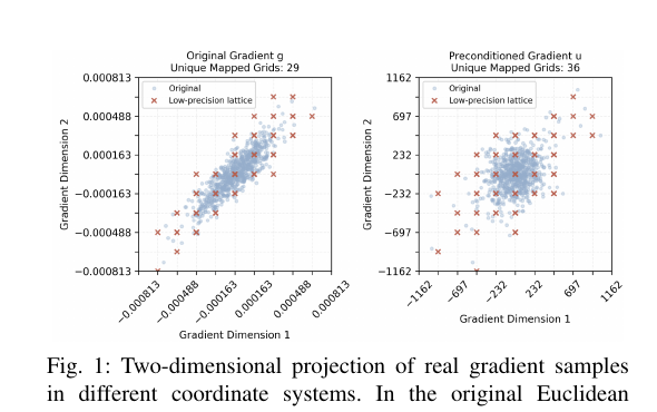
This figure is the direct visual counterpart of Eq. (9): the left panel is the raw $\Delta W$ space, where the K-FAC ellipsoid $\{\Delta W : \|\Delta W\|_{F_W}^2 \le \epsilon\}$ is genuinely stretched (some directions have far larger K-FAC-weighted “importance” than others even at equal Euclidean magnitude); the right panel is the $U$-space after applying $U = L_G^\top \Delta W\, L_A$, where that same ellipsoid becomes (by construction, via Eq. 9’s algebra) a round ball. A uniform, axis-aligned FP8 quantization grid is a poor match for the left panel’s geometry — it must simultaneously accommodate the long axis (risking clipping) and the short axis (wasting most of its representable levels on a direction that barely varies) — but is a good match for the right panel’s geometry, where every axis has comparable spread. In other words, define

$$U = L_G^\top\, \Delta W\, L_A, \tag{10}$$

then the original ellipsoid constraint $\{\Delta W : \|\Delta W\|_{F_W}^2 \le \epsilon\}$ maps exactly onto the round Euclidean ball $\{U : \|U\|_F^2 \le \epsilon\}$. This is why the transform is called “whitening”: it takes a correlated, direction-dependent (anisotropic) object and maps it into an uncorrelated, direction-independent (isotropic) one — the same core idea as whitening a colored-noise signal in classical signal processing.

Step 3: Applying Whitening to Communication, Not Optimization

The insight above is about perturbations to weights, but GIFT needs it applied to gradients being communicated. The paper defines the full geometry-informed communication coordinate for a gradient $W_g$ as

$$\widetilde{W}_g = L_G^{-1}\, W_g\, L_A^{-\top}. \tag{11}$$

Why the inverse factors here, rather than the same factors as in Eq. (10)? Because Eq. (10) was whitening a perturbation being measured against the metric — you multiply by the geometry factors to map a Euclidean ball onto an ellipsoid-shaped perturbation. Here we’re doing the reverse job: we have a gradient that already “lives” in a coordinate system where the meaningful metric is the anisotropic K-FAC ellipsoid, and we want to re-express it in coordinates where the plain Euclidean metric matches what used to be the K-FAC metric — i.e., we want to undo the anisotropy before quantizing with a uniform Euclidean-style scale. That requires the inverse factors, $L_G^{-1}$ and $L_A^{-\top}$, applied on the appropriate sides. Equivalently, in vectorized form:

$$\mathrm{vec}(\widetilde W_g) = \left(L_A^{-1} \otimes L_G^{-1}\right) \mathrm{vec}(W_g), \tag{12}$$

which removes the dominant input-side scaling (captured by $A$, via $L_A^{-1}$) and output-side scaling (captured by $G$, via $L_G^{-1}$) from the gradient before it is quantized. In these transformed coordinates, the gradient distribution is closer to isotropic, so an axis-aligned FP8 quantization grid — which fundamentally treats every coordinate the same way — interacts with the gradient far more uniformly than it does in the raw, anisotropic Euclidean coordinates.

After this whitening, GIFT applies the exact same low-precision communication procedure any Euclidean-space scheme would use — scale, quantize to FP8, all-reduce, dequantize, average:

$$\widehat{\widetilde W}_g = \mathrm{CommFP8}\!\left(\widetilde W_g\right), \tag{13}$$

and then maps the synchronized, dequantized result back to the original Euclidean gradient coordinates before the optimizer ever touches it:

$$\widehat{W}_g = L_G\, \widehat{\widetilde W}_g\, L_A^\top. \tag{14}$$

This final map-back step is what makes GIFT strictly a communication-time technique rather than an optimizer change: $\widehat{W}_g$ lands right back in the space the optimizer expects, so the same FP32/BF16 Muon (or Adam, or any other) optimizer update can be applied unmodified. Nothing about the model architecture, the distributed-parallelization strategy, or the optimizer update rule is touched — only the coordinate system momentarily used for communication changes.

Why “Not a K-FAC Optimizer” Is a Genuine Design Choice, Not Just a Caveat

It’s worth pausing on why the paper insists so explicitly that GIFT is not a K-FAC-style natural-gradient method, because this is a real design decision with real tradeoffs, not just a disclaimer. A true K-FAC optimizer would apply the preconditioner $F^{-1}$ to every gradient at every step and feed the transformed gradient into the optimizer’s update rule — changing the optimization trajectory itself, for better or worse (K-FAC-preconditioned training can converge faster per-step but each step is more expensive, and the approximation quality of the block-diagonal Kronecker structure directly affects whether the resulting trajectory is actually better). GIFT sidesteps all of that: because the transform is undone (Eq. 14) before the optimizer sees anything, the optimization dynamics are provably unchanged relative to the Euclidean baseline — the only thing that changes is how faithfully the averaged gradient survives its round-trip through FP8. This is a genuinely clean separation of concerns: it means any accuracy differences observed between GIFT and Euclidean baseline in the experiments can be attributed specifically to communication fidelity, not to some entangled effect of a different optimization trajectory. The boundary case where this choice could fail is if the K-FAC factors are so stale or so poorly estimated that the “whitening” transform actually increases variance in some direction rather than decreasing it — we come back to this in the critical-assessment section, because the paper’s factor-refresh schedule (every 50 steps) is a real, underexamined risk here.

From Theory to Practice: Three Simplifications

The full two-sided transform (Eq. 11) is conceptually clean but, applied to every eligible layer at every step, is too expensive for real LLM pretraining: computing and Cholesky-factoring both $A \in \mathbb{R}^{d_\text{in}\times d_\text{in}}$ and $G \in \mathbb{R}^{d_\text{out}\times d_\text{out}}$ for every layer, every refresh period, adds real compute and memory. Section V of the paper systematically strips this down through three simplifications, each justified by a targeted ablation before being adopted — a methodologically careful pattern worth explaining step by step, because it’s the difference between “we guessed this would be cheaper” and “we measured that this specific simplification loses almost nothing.”

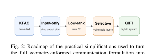
This roadmap is worth keeping in view while reading the next three subsections: each box represents one deliberate reduction in scope, and each arrow represents a targeted experiment (Table I, Table II, and the Figure 3 profiling study respectively) that the paper runs before committing to the simplification, rather than simplifying first and hoping the accuracy holds up. The end state — bottom of the roadmap — is the selective, input-side-only, rank-32 design that Algorithm 1 formalizes below.

Simplification 1: Input-Side Only

The question: which side of the two-sided transform — the input-side factor $L_A$ or the output-side factor $L_G$ — is actually responsible for the practical fidelity gain?

The experiment: a controlled one-step FP8 round-trip test. Start from an FP32 gradient $g$, map it into a candidate set of communication coordinates, apply a single FP32→FP8→FP32 round trip in those coordinates, map the result back to Euclidean gradient space, and compare the reconstructed gradient $\hat g$ against the original $g$ using four metrics:

$$\mathrm{RelL2} = \frac{\|\hat g - g\|_2}{\|g\|_2}, \qquad \mathrm{Cos} = \frac{\langle \hat g, g\rangle}{\|\hat g\|_2 \|g\|_2}, \qquad \mathrm{MaxErr} = \|\hat g - g\|_\infty, \qquad \mathrm{MSE} = \frac{\|\hat g - g\|_2^2}{n}. \tag{15}$$

RelL2, MaxErr, and MSE are all “lower is better” magnitude-of-error measures at different sensitivities (RelL2 is a normalized average-case measure, MaxErr captures the single worst-affected entry, MSE emphasizes large errors quadratically); Cos measures whether the FP8 round trip preserves the gradient’s direction — arguably the most important property for optimization, since gradient descent primarily cares about which way you’re stepping.

The result (paper’s Table I): the output-side-only transform is essentially indistinguishable from the plain Euclidean baseline across all four metrics (RelL2 $5.283\times10^{-2}$ vs. baseline’s $5.282\times10^{-2}$) — it contributes almost nothing. The input-side-only transform, in contrast, nearly matches the full two-sided K-FAC transform on every metric (RelL2 $1.768\times10^{-2}$ for input-side vs. $1.771\times10^{-2}$ for full K-FAC — a difference in the fourth significant figure). This is a genuinely useful empirical finding, not an obvious one a priori: it says that for this particular Muon-optimized Llama setup, essentially all of the anisotropy that matters for FP8 fidelity lives on the input-activation side of each layer, not the output-gradient side. The design conclusion: drop the output-side transform entirely and keep only

$$\widetilde W_g = W_g\, T_A, \tag{16}$$

where $T_A$ is the input-side transform derived from $L_A^{-1}$ (in the input-side-only reduction of Eq. 11’s $L_A^{-\top}$ term). This alone roughly halves the geometric machinery that needs to be computed and stored per layer, since $G$ and its Cholesky factor $L_G$ are no longer needed at all.

Why might this be true, and what’s the boundary? One plausible mechanistic explanation: for MLP layers (the paper’s profiling target, see Simplification 3 below), the input activations $a$ feeding into a layer are shaped by the entire upstream network — normalization statistics, prior nonlinearities, residual accumulation — and can develop substantially correlated, elongated structure across the batch dimension. The output-gradient $\delta$, on the other hand, is a backpropagated signal that has already been smoothed by the chain rule through many downstream layers, and empirically may be closer to isotropic by the time it reaches any given layer. This is a hypothesis the paper doesn’t explicitly test (it reports the result but doesn’t dig into why input-side dominates), which is worth flagging: it’s entirely plausible this asymmetry is specific to the Muon optimizer, this depth/width regime, or this particular pretraining recipe, and would not transfer unchanged to, say, attention-layer gradients or a different optimizer’s gradient statistics.

Simplification 2: Rank-32 Low-Rank Approximation

The question: once you’ve committed to only the input-side factor $A$, how accurately does it actually need to be represented? Using the full $d_\text{in}\times d_\text{in}$ matrix $A$ (and its Cholesky factor) for every selected layer is still expensive to store and compute.

The setup: write $A \approx \mathbb{E}[xx^\top]$ (a positive semi-definite second-moment matrix, $A \succeq 0$), and consider its low-rank eigendecomposition approximation

$$A \approx U_r \Lambda_r U_r^\top, \tag{17}$$

keeping only the top $r \ll d_\text{in}$ eigenvectors/eigenvalues. Constructing the input-side transform from this reduced representation instead of the full $A$ dramatically cuts both the storage (only $r$ vectors of length $d_\text{in}$ instead of a full $d_\text{in}\times d_\text{in}$ matrix) and the compute cost of applying the transform.

The result (paper’s Table II): a diagonal approximation of $A$ (i.e., treating $A$ as if it had no cross-dimension correlations at all — just per-dimension variance) barely improves over the untransformed Euclidean baseline (RelL2 $5.262\times10^{-2}$ vs. baseline $5.282\times10^{-2}$ — essentially no gain). This is an important negative result: it directly demonstrates that the benefit of geometry-awareness comes from the off-diagonal, cross-dimension correlation structure of $A$, not merely from re-scaling each individual coordinate by its own variance. A naive “just normalize each dimension by its own magnitude” scheme — which might seem like an obvious cheap approximation to try — would essentially not help at all here. In contrast, low-rank approximations of the full matrix recover almost all of the benefit: rank-8 gets RelL2 $1.958\times10^{-2}$, rank-16 gets $1.731\times10^{-2}$, and rank-32 gets $1.721\times10^{-2}$ — essentially matching the full-$A$ result of $1.768\times10^{-2}$ while being far cheaper to store and apply. The paper settles on rank-32 “as the operating point for our implementation rather than as a model-independent constant” — an honest acknowledgment that this specific number is a tuned hyperparameter for this specific setup, not a universal law.

Why does this pattern make sense? The intuition is that the “interesting” anisotropic structure in activation statistics is usually concentrated in a handful of dominant directions (e.g., a few directions where activations are systematically large due to some combination of layer normalization scale, residual-stream magnitude growth with depth, or a handful of highly-active “outlier” feature dimensions that are well-documented in the LLM quantization literature more broadly), with a long tail of directions that behave close to isotropically already. A low-rank correction targeting just the dominant directions captures most of the useful whitening effect, while the diagonal approximation — which can only rescale individual axes, never mix or rotate between them — cannot correct for correlation between dimensions at all, which is exactly where the paper’s diagonal-approximation result shows it fails.

Simplification 3: Selective Deployment on Vulnerable Layers Only

The question: even with input-side-only and rank-32, applying the geometry-aware branch to every layer in the model still adds meaningful overhead. Do all layers actually need it?

The profiling procedure: run the plain Euclidean-baseline pretraining for the first 100 training steps on a 32-GPU, 600M-parameter run, and for every MLP layer (both fc1 and fc2 sub-layers), flatten its gradient tensor, compute the FP8 quantization scale that would be used, encode the flattened gradient into FP8, and count how often the encoded values hit the FP8 format’s upper or lower representable boundary (i.e., saturate/clip rather than round to an interior value). Average these boundary-hit ratios over the 100-step profiling window separately for fc1 and fc2 layers, sum the upper- and lower-boundary hit rates per layer, and use this sum as a numerical-vulnerability score — a direct, cheap, model-agnostic proxy for “how much is this layer’s gradient actually being distorted by FP8 quantization under the Euclidean baseline right now.”

The finding (Figure 3): vulnerability is highly concentrated. In the 600M-model profile, the top 13 most vulnerable layers are all fc2 layers (the second linear layer inside each MLP block, i.e., the one that projects back down from the expanded hidden dimension), and there is a visible drop in vulnerability score right after this group — the 14th-ranked layer (the first fc1 layer in the ranking) sits noticeably lower. The number 13 is explicitly not claimed as a universal constant; it’s simply “the operating point selected by the vulnerability-ranking procedure for this model and recipe,” and the same profiling procedure “can be rerun automatically to select the layer set” for a different architecture.

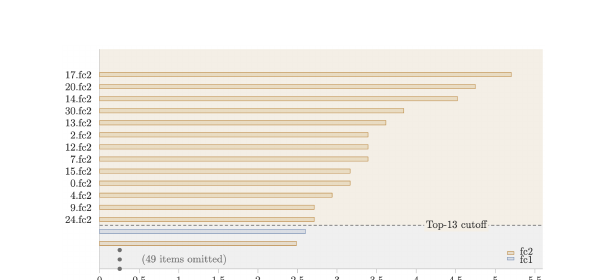
The shape of this curve is exactly what justifies a hard cutoff rather than a continuous, graded deployment: vulnerability isn’t smoothly spread across all layers, it’s concentrated in a distinct group followed by a visible “elbow” drop. That elbow is what the paper’s selection rule (“take the layers before the visible score drop”) operationalizes into a concrete layer set $S$.

The design: enable the geometry-aware (input-side, rank-32) branch only on this profiled vulnerable-layer set $S$, and leave every other layer on the plain Euclidean fast path. This is the crux of GIFT’s practicality: rather than a heavy, uniform geometry-aware system applied everywhere (like a full K-FAC state per layer, which the paper shows is both more expensive and slightly worse on downstream tasks than the selective design — see Table III’s 300M “Full K-FAC” row scoring 6/14 wins vs. FP32, below GIFT’s 7/14), GIFT is a hybrid: most of the model stays exactly as cheap as the Euclidean baseline, and the extra machinery is concentrated only where the profiling data says it actually helps.

Why might fc2 layers specifically be the most vulnerable? A plausible mechanistic reason, though the paper doesn’t spell it out explicitly: the fc2 sub-layer’s input activations are the outputs of the MLP’s nonlinearity (e.g., GELU/SiLU applied to the expanded hidden representation), which are known in the broader quantization literature to develop heavy-tailed, highly non-uniform activation statistics — a small number of “hot” feature channels can carry disproportionately large magnitudes compared to the rest. If this is the mechanism, it directly explains why fc2’s input-side geometry ($A$, from Simplification 1) specifically benefits from whitening, and connects back to why Simplification 1 found the input side (not the output side) to matter most.

This connects to a broader, well-documented phenomenon in the LLM quantization literature sometimes called “activation outliers” or “massive activations”: across many transformer architectures, a small number of specific hidden dimensions (often associated with particular attention-sink or bias-like behaviors that emerge during training) develop activation magnitudes many times larger than the typical dimension, concentrated especially in certain MLP sub-layers and certain depths of the network. If GIFT’s fc2-concentrated vulnerability profile reflects the same underlying phenomenon, that would suggest the specific layer-selection pattern (concentrated in fc2, not spread uniformly) is not an accident of this particular Llama/Muon/OpenWebText recipe but a more structural property of transformer MLP blocks under FP8 quantization — a hypothesis the paper’s own profiling data is consistent with but does not explicitly test against the broader outlier-activation literature it doesn’t cite in this context.

A Note on Why Selective Deployment Beats Uniform Deployment, Even Setting Aside Cost

It would be easy to assume the only reason GIFT restricts the geometry-aware branch to a subset of layers is to save compute and memory — and that’s certainly part of it. But Table III’s finding that the selective GIFT design out-performs the heavier full-K-FAC-everywhere variant (7/14 vs. 6/14 wins at 300M) points to a second, independent reason: applying an estimated correction to a layer that doesn’t actually need it can be a net negative, not merely a wasted expenditure. Every K-FAC factor $A^{(l)}$ used in the whitening transform is itself an empirical estimate — computed from a finite window of training data, refreshed only every 50 steps — and estimation noise in that factor gets baked directly into the whitening transform applied to that layer’s gradient. For a layer whose gradients are already close to isotropic (i.e., a layer that wouldn’t benefit much from whitening in the first place), applying a noisy estimate of a nearly-trivial correction can introduce more distortion than it removes, essentially injecting estimation noise into a signal that didn’t have much of a shape problem to begin with. This is a coherent, if implicit, explanation for why “more geometric correction, applied everywhere” underperforms “less geometric correction, applied only where the profiling data says it’s needed” — and it means the selective-deployment design isn’t just a systems-efficiency compromise, it’s plausibly better on accuracy grounds too, which is a stronger and more interesting claim than the paper states explicitly.

Putting It Together: The Full Selective GIFT Algorithm

The paper’s Algorithm 1 formalizes the complete per-step, per-layer communication rule combining all three simplifications, plus one detail not yet discussed: error feedback. Here it is, restated with a line-by-line walkthrough:

Algorithm 1: Selective GIFT Communication with Input-Side Whitening and Error Feedback

Require: Fixed selected layer set S (from offline profiling, Simplification 3)
Require: For each l in S, input-side factorization A^(l) ≈ L_A^(l) (L_A^(l))^T,
         refreshed every K = 50 training steps
Require: Error buffers {R^(l)}_{l in S}, initialized to zero
Require: World size N, FP8 quantizer Q(·; s), scaling rule Scale(·)

 1: for each training step do
 2:     for each layer l with weight gradient W_g^(l) do
 3:         if l not in S:                                  # plain Euclidean fast path
 4:             s^(l) <- Scale(W_g^(l))
 5:             s^(l) <- AllReduceMax(s^(l))                 # synchronize scale across workers
 6:             Q^(l) <- Q(W_g^(l); s^(l))                   # quantize to FP8
 7:             Q_hat^(l) <- AllReduceSum(Q^(l))              # all-reduce the quantized values
 8:             W_hat_g^(l) <- Dequantize(Q_hat^(l); s^(l)) / N
 9:         else:                                            # geometry-aware branch
10:             U^(l) <- W_g^(l) . (L_A^(l))^{-T}              # input-side whitening transform
11:             U_tilde^(l) <- U^(l) + R^(l)                  # add carried-over error feedback
12:             s_loc^(l) <- Scale(U_tilde^(l))                # local scale in whitened coords
13:             Q_tilde^(l) <- Q(U_tilde^(l); s_loc^(l))       # quantize whitened gradient
14:             U_tilde_deq^(l) <- Dequantize(Q_tilde^(l); s_loc^(l))
15:             R^(l) <- U_tilde^(l) - U_tilde_deq^(l)         # update error-feedback buffer
16:             s_comm^(l) <- s_loc^(l)
17:             if this is a scale-synchronization step:
18:                 s_comm^(l) <- AllReduceMax(s_loc^(l))      # occasionally sync scales too
19:             end if
20:             Q_hat^(l) <- AllReduceSum(Q_tilde^(l))
21:             U_hat^(l) <- Dequantize(Q_hat^(l); s_comm^(l)) / N
22:             W_hat_g^(l) <- U_hat^(l) . L_A^(l),T           # map back to Euclidean coordinates
23:         end if
24:     end for
25:     Optimizer updates parameters using {W_hat_g^(l)}
26: end for

Walking through the two branches:

• Lines 3-8 (non-selected layers): this is exactly the standard Euclidean FP8 all-reduce that any baseline low-precision scheme would run — compute a local scale, synchronize the scale across workers (so everyone quantizes using the same reference scale), quantize, all-reduce the quantized integer/FP8 values (summing them), dequantize, and divide by the world size $N$ to get the averaged gradient. No geometry involved.
• Line 10 (whitening): for a selected layer, the gradient is first right-multiplied by $(L_A^{(l)})^{-\top}$ — this is the input-side-only reduction of the full transform in Eq. (11)/(16), applied per-layer using that layer’s own K-FAC factor.
• Lines 11-15 (error feedback): rather than quantizing the whitened gradient $U^{(l)}$ directly, GIFT first adds a carried-over error-feedback residual $R^{(l)}$ from the previous step, quantizes the sum, and then computes the new residual as the difference between the pre-quantization and post-dequantization values. This is a well-established technique from the broader gradient-compression literature (used in methods like DGC and 1-bit Adam, both cited by the paper): instead of discarding whatever a single quantization step rounds away, you accumulate that rounding error locally and re-inject it at the next step, so that systematic quantization bias doesn’t compound silently over many steps — it eventually gets folded back in rather than permanently lost. Applying error feedback in the whitened coordinates (rather than treating it as an unrelated post-hoc correction in Euclidean space) keeps this technique consistent with the rest of the communication formulation.
• Lines 16-19 (scale synchronization): the local scale $s_\text{loc}^{(l)}$ computed from each worker’s own (locally different) gradient is normally used as-is for that worker’s own quantization step, but on designated “scale-synchronization steps,” the paper instead all-reduces the maximum local scale across workers first, so everyone quantizes against a common reference scale — a standard tradeoff between per-worker scale accuracy (using each worker’s own local scale saves a synchronization round trip) and cross-worker scale consistency (using a globally agreed scale avoids subtly different rounding behavior per worker). The paper notes local scaling in transformed coordinates “gives better empirical fidelity than synchronizing a global scale in our ablation” — i.e., the default mode favors per-worker local scales, with global synchronization used only periodically.
• Lines 20-22 (all-reduce and map-back): the quantized whitened values are all-reduced and dequantized exactly as in the plain path, and then — critically — mapped back to Euclidean coordinates via right-multiplication by $L_A^{(l),\top}$, so that whatever downstream code consumes $\widehat W_g^{(l)}$ (the optimizer) never has to know the geometry-aware branch existed at all.

Two implementation notes the paper emphasizes: first, the geometry-aware branch is genuinely only active on the small fixed subset $S$, so the majority of the model’s communication code path is byte-for-byte identical to the plain baseline; second, error feedback happens in the transformed coordinates specifically, which the paper argues keeps it “aligned with the communication formulation rather than treating error feedback as a separate post hoc correction” — a design-consistency argument rather than a measured ablation, worth noting as a place where the paper asserts a design principle without a side-by-side comparison against “error feedback in Euclidean space after mapping back.”

Computational Complexity: What the Selective Design Actually Buys You

It’s worth making the cost accounting in Algorithm 1 explicit, because “selective deployment” is a specific, quantifiable claim, not just a qualitative one. Consider a linear layer with weight $W \in \mathbb{R}^{d_\text{out}\times d_\text{in}}$.

Cost of the non-selected (plain Euclidean) path, lines 3-8: computing a scale is $O(d_\text{out} d_\text{in})$ (one pass over the tensor to find the max absolute value), quantization is another $O(d_\text{out} d_\text{in})$ elementwise pass, and the all-reduce communicates $d_\text{out} d_\text{in}$ FP8 values (1 byte each, versus 4 bytes for FP32) — this is the baseline cost every method in this comparison pays.

Additional cost of the selected (geometry-aware) path, lines 10-22, on top of the baseline: the whitening transform $U^{(l)} = W_g^{(l)} L_A^{(l),-\top}$ is a matrix product of a $d_\text{out}\times d_\text{in}$ matrix with a $d_\text{in}\times d_\text{in}$ matrix, costing $O(d_\text{out} d_\text{in}^2)$ if done with the full factor — this is exactly why the rank-32 approximation (Simplification 2) matters computationally, not just for storage: applying a rank-$r$ factorization instead reduces this to $O(d_\text{out} d_\text{in} r)$, which for $r=32 \ll d_\text{in}$ (typical MLP hidden dimensions run into the thousands) is a substantial reduction — potentially 1-2 orders of magnitude cheaper than the full-rank transform, depending on $d_\text{in}$. The map-back transform (line 22) costs the same $O(d_\text{out} d_\text{in} r)$ by symmetry. The error-feedback bookkeeping (lines 11, 15) is $O(d_\text{out} d_\text{in})$, same order as the baseline quantization step, so it doesn’t change the asymptotic picture.

Factor maintenance cost, amortized: computing $A^{(l)} \approx \mathbb{E}[aa^\top]$ from a batch of activations costs $O(N_\text{batch} \cdot d_\text{in}^2)$ if done directly, then a rank-$r$ eigendecomposition of that $d_\text{in}\times d_\text{in}$ matrix costs roughly $O(d_\text{in}^2 r)$ using an iterative method (e.g., randomized SVD or power iteration, standard for extracting a handful of leading eigenvectors from a matrix too large to fully diagonalize cheaply). Since this only happens once every $K=50$ steps, its amortized per-step cost is this total divided by 50 — small relative to the per-step whitening/map-back cost, provided $d_\text{in}$ isn’t enormous, but not free, especially since the paper doesn’t report how this factor-computation cost is distributed (synchronously blocking the training step, or overlapped/asynchronous with other work) — a gap flagged again in the critical-assessment section below.

Putting this together: for a layer not in $S$, GIFT’s cost is identical to the Euclidean baseline. For a layer in $S$, GIFT adds roughly $O(d_\text{out} d_\text{in} r)$ per step for the transform pair, plus an amortized $O(d_\text{in}^2 r / K)$ for factor maintenance — and because $|S|$ (13 layers in the paper’s 600M profile) is a small fraction of the total layer count, the aggregate extra cost across the whole model stays bounded, which is exactly the systems argument the 3.33%/8.98% memory overhead numbers (Section VI-E) and the Figure 5 timing curves are empirically confirming.

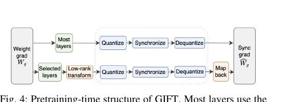
This figure is the systems-level picture of exactly what Algorithm 1 describes in pseudocode: a single shared “communication core” (quantize → all-reduce → dequantize) that every layer passes through, with the geometry-aware branch drawn as an optional detour — a whitening transform before the core and a map-back transform after it — that only the selected vulnerable layers take. The diagram makes visually explicit why GIFT’s overhead is bounded: the expensive detour is architecturally confined to a small subset of the graph, not smeared across every edge.

Experimental Results

The paper evaluates GIFT from four angles: systems-level scaling benefit, validation-loss preservation, downstream task-quality preservation, and memory overhead.

Experimental Setup

Two LLaMA-style pretraining configurations on OpenWebText: a ~300M-parameter model at sequence length 4096, and a ~600M-parameter model at sequence length 2048 (different sequence lengths chosen to fit GPU memory constraints, not as an independent experimental variable). Unless stated otherwise, end-to-end runs use 32 GPUs, global batch size 512, micro batch size 4, the Muon optimizer, learning rate $5\times10^{-4}$ with cosine decay down to a minimum of $5\times10^{-5}$. All experiments run on the Vista supercomputer at TACC, using NVIDIA GH200 Grace Hopper Superchip nodes (96GB HBM3 per GPU, tightly integrated CPU-GPU design).

A methodologically careful choice worth flagging explicitly: the paper doesn’t just compare GIFT against a single “Euclidean FP8” baseline — it first runs additional 600M-scale experiments to determine which baseline variant is actually strongest, so the main comparison isn’t accidentally stacked against a weak baseline. It finds BF16 gradient communication matches FP32 on 7/14 downstream tasks but has slightly lower absolute task values overall (so FP32 remains the reference); per-block Euclidean FP8 (block size 512) matches FP32 on only 4/14 tasks, worse than layer-wise Euclidean FP8’s 5/14 — so the paper uses the stronger layer-wise Euclidean FP8 as its main baseline throughout, rather than a weaker straw-man variant.

Systems Benefit: Scaling With GPU Count (Figure 5)

Figure 5 plots step-time improvement over an FP32 baseline (positive = faster than FP32, negative = slower) as GPU count increases, for both the 300M and 600M models, comparing the Euclidean FP8 baseline and GIFT. Three observations:

1. Low-precision communication’s advantage grows with scale — the relative speedup over FP32 becomes more pronounced at higher GPU counts, especially for the 600M model, because communication occupies a larger fraction of total step time as the model and cluster scale grow (more parameters to synchronize, more workers to synchronize across).
2. GIFT is consistently slower than the plain Euclidean baseline, because it introduces extra geometry-aware computation (the whitening transform, the map-back transform, and the Cholesky-factor maintenance every 50 steps) — this is an honest, expected cost, not something the paper tries to hide.
3. Critically, GIFT still retains a substantial fraction of the low-precision speedup relative to FP32, and the gap between GIFT and the Euclidean baseline’s speedup widens as GPU count increases — meaning at the largest scales tested, communication efficiency matters most and GIFT’s extra overhead becomes relatively less consequential as a fraction of total savings.

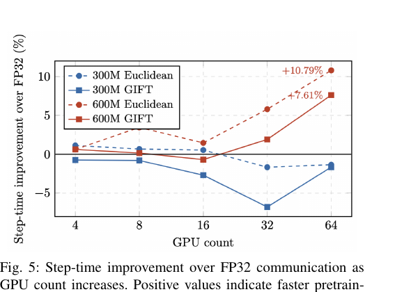
Reading this figure carefully: both curves (Euclidean baseline and GIFT) trend upward (more speedup vs. FP32) as GPU count increases, and the vertical gap between the two curves is the systems cost GIFT pays for its downstream-quality advantage. The paper’s argument is that this vertical gap does not grow proportionally as fast as the curves themselves rise — i.e., GIFT’s absolute overhead is roughly fixed per step, while the baseline communication savings it’s riding on top of keep growing with scale, so GIFT’s overhead becomes a shrinking fraction of the total picture at the largest scales tested.

Validation Loss: A Deliberately Unexciting Result (Figure 6)

Figure 6 compares FP32, Euclidean baseline, and GIFT validation-loss trajectories during pretraining, for both model sizes.

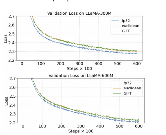
The headline finding here is almost anticlimactic: GIFT and the Euclidean baseline produce nearly indistinguishable validation-loss curves, both staying reasonably close to the FP32 reference throughout training. The paper treats this as an important methodological point rather than a disappointing result: it argues that validation loss, while a useful signal, is an incomplete proxy for the effect of communication-coordinate choice on the model’s actual downstream usefulness — the differences between communication schemes “may become more apparent in downstream performance than in pretraining loss alone.” This sets up the paper’s main empirical claim, which lives in the downstream task table, not the loss curve.

Downstream Task Performance: Where the Signal Actually Shows Up (Table III)

Table III reports per-task downstream accuracy across 14 diverse tasks (BOOLQ, CB-ACC, COPA, MUL-RC, RCD-F1, RTE, WiC, WSC, LAMBADA, RACE, M-QA, PIQA, WinoGrande, LAMBADA-standard), for FP32, BF16, per-block Euclidean FP8, layer-wise Euclidean FP8, full K-FAC, and GIFT, at both 300M and 600M scale. The summary metric the paper emphasizes is “wins vs. FP32” — the count of tasks on which a method’s accuracy exceeds the FP32 reference’s accuracy:

Model	Method	Wins vs. FP32 (out of 14)
600M	BF16	7
600M	Per-block Euclidean FP8	4
600M	Layer-wise Euclidean (main baseline)	5
600M	GIFT	7
300M	Layer-wise Euclidean (main baseline)	4
300M	Full K-FAC	6
300M	GIFT	7

At both scales, GIFT wins on 7/14 tasks, clearly ahead of the layer-wise Euclidean baseline (5/14 at 600M, 4/14 at 300M), and — notably — ahead of the heavier full K-FAC variant tested at 300M (6/14), which uses the complete two-sided transform on every eligible layer rather than GIFT’s selective, input-side-only, rank-32 design. This last comparison is the paper’s strongest single piece of evidence for its “selective, simplified” design philosophy: doing more geometry-aware computation everywhere is not just more expensive, it actually does worse than doing less geometry-aware computation in a targeted way — plausibly because the full K-FAC state, estimated and refreshed under the same practical constraints (limited profiling window, periodic refresh), introduces its own estimation noise on layers where the geometric correction wasn’t needed in the first place, without buying anything back in return.

The paper is careful to frame this correctly: “these results should not be interpreted as GIFT matching FP32 on every task” — no method does, and task-by-task results are genuinely mixed (looking at the raw numbers in Table III, GIFT loses to the Euclidean baseline on some individual tasks even while winning the aggregate “wins vs. FP32” count, e.g. 600M CB-ACC: Euclidean 0.4107 vs. GIFT 0.3036). The claim is specifically about the cross-task preservation profile — GIFT more consistently stays close to or above the FP32 reference across the task suite as a whole, not that it dominates every individual task.

Memory Overhead (Section VI-E)

GIFT increases memory usage by 3.33% for the 300M model and 8.98% for the 600M model, relative to the Euclidean baseline. This overhead comes from storing the rank-32 low-rank input-side factors and the error-feedback residual buffers, but only for the small selected-layer subset $S$ — the paper explicitly frames this as staying “limited rather than scaling as a full two-sided per-layer K-FAC state,” reinforcing why the selective-deployment design (Simplification 3) matters for practicality, not just for the accuracy result discussed above.

End-to-End Systems Payoff: 7.6% Time Reduction, Explicitly Smaller Than the Baseline’s 10.79%

Putting the pieces together at the full pretraining scale (64 GH200 superchips, Llama-600M): GIFT reduces gradient communication payload size by 75.0% relative to FP32 (the mechanical consequence of using FP8 instead of FP32, same as any FP8 scheme would achieve), which translates into a 7.6% reduction in end-to-end pretraining time. The paper is unusually direct about the fact that this is smaller than the plain Euclidean FP8 baseline’s own 10.79% reduction at the same scale — GIFT explicitly trades away some of the raw communication-time speedup in exchange for the better downstream-preservation profile documented in Table III. Whether this tradeoff is worth it depends entirely on how much a practitioner values the last few points of task-preservation quality against pretraining wall-clock time — a genuine cost-benefit question the paper poses rather than resolves for the reader. The paper also makes an argument about why even a modest percentage matters at scale: modern LLMs are pretrained across tens of thousands of GPUs over months, so “even a 7.6% reduction in time can translate to millions of dollars,” and freed-up interconnect bandwidth is itself a valuable shared resource as compute scales faster than interconnect bandwidth.

Frequently Confused Points

A few aspects of GIFT’s design are easy to conflate with superficially similar ideas; this section addresses the most likely points of confusion directly.

“Isn’t this just K-FAC?” No — K-FAC as an optimizer uses $F^{-1}$ (or an approximation to it) to precondition the gradient before the parameter update, permanently changing the optimization trajectory relative to plain SGD/Adam/Muon. GIFT uses the same factorization ($A \otimes G$) but only as a temporary change of basis around the communication step (Eqs. 11-14): the gradient is mapped into whitened coordinates, quantized, communicated, and mapped straight back — by the time the optimizer sees it, it’s numerically (up to quantization error) the same gradient it would have been under the plain Euclidean scheme. The optimization trajectory is unchanged; only the fidelity of the averaged gradient after its FP8 round-trip changes.

“Doesn’t whitening the gradient change what the model learns?” Not in the way natural-gradient methods do. Because the transform in Eq. (14) exactly inverts the transform in Eq. (11) (modulo the FP8 quantization noise introduced in between), the net effect on the optimizer’s input is: same gradient, but with a different (hopefully smaller) FP8-induced perturbation. If GIFT used a lossless communication format (e.g., if it communicated in FP32 through the whitened coordinates), the map-back would be a mathematical identity and GIFT would be provably equivalent to the plain baseline. The only reason GIFT’s whitened coordinates matter at all is that quantization to a lossy, narrow format like FP8 happens in between the forward and inverse transforms — whitening only changes how much information the FP8 round-trip destroys, not what the gradient represents.

“Why not just use a diagonal (per-dimension) scale instead of the full geometric transform?” This is precisely the ablation Table II answers: a diagonal approximation of $A$ barely improves over the untransformed Euclidean baseline (RelL2 $5.262\times10^{-2}$ vs. baseline’s $5.282\times10^{-2}$), because a diagonal matrix can only rescale individual coordinate axes, never rotate or mix between them — and the paper’s evidence (contrasted against the much larger gain from even a rank-8 low-rank approximation) is that the useful part of the anisotropy correction specifically requires correcting cross-dimension correlation, which a purely diagonal (per-axis) scale is mathematically incapable of representing.

“Does GIFT require every worker to compute its own K-FAC factors, or is there a single shared factor?” The paper’s algorithm (line “Require: For each l in S, input-side factorization… refreshed every K steps”) implies a factor per layer, refreshed periodically; it doesn’t explicitly clarify whether this factor is computed locally per-worker from that worker’s own activation batch, or computed from a globally-aggregated activation statistic and then broadcast/synchronized across workers. This is a real implementation detail that affects both the fidelity of the factor (a globally-aggregated $A$ would presumably better represent the “true” population statistics than any single worker’s local batch) and the synchronization cost of maintaining it (a globally-synchronized factor needs its own periodic collective communication, separate from the gradient all-reduce) — and the paper’s presentation leaves this ambiguous, which is worth flagging as a gap for anyone attempting to reproduce the exact system.

Limitations (As Stated by the Authors)

The paper explicitly names three limitations in its own “Limitations” section:

1. Scale: end-to-end experiments are limited to two medium-scale (300M/600M parameter) Llama models under a fixed pretraining recipe; testing larger models, longer training horizons, and broader hardware regimes is left to future work.
2. Evaluation breadth: while downstream results already show a consistent GIFT-over-Euclidean advantage, the paper notes this would be “further strengthened by additional seeds and a larger benchmark suite” — an acknowledgment that the current 14-task, apparently single-seed comparison has real statistical uncertainty attached to it that isn’t quantified anywhere in the paper.
3. Scope of the compression stack: this work is communication-only low-precision compression, not a fully quantized pretraining stack (it doesn’t touch weights, activations, or optimizer states) — whether the geometry-aware principle remains useful when combined with those other forms of low-precision pretraining is explicitly left open.

Critical Assessment: Weaknesses & Improvements

Weaknesses & Flaws

• Single-seed uncertainty on downstream results. Table III presents point estimates for 14 downstream tasks with no reported variance, confidence intervals, or multiple-seed averaging. Several of the reported “wins” are narrow — e.g. at 600M, GIFT’s WiC score (0.5031) vs. the Euclidean baseline’s (0.4969) is a 0.62-point gap on a task that is itself a binary-ish word-sense classification benchmark with substantial run-to-run noise typically reported in the broader literature. Without seeds or variance bars, it’s genuinely unclear how many of the individual per-task differences in Table III would survive a repeat run, even though the aggregate “wins vs. FP32” pattern (7 vs. 4-5) is a large enough gap that it plausibly would.
• The K-FAC factor refresh schedule (every 50 steps) is asserted, not ablated. The paper reports this as a fixed hyperparameter without showing what happens at, say, every-10-steps (fresher, more expensive) or every-200-steps (staler, cheaper) refresh — leaving open whether 50 is close to optimal or simply “the first value tried that worked well enough.” Given that the whole method rests on the K-FAC factors being a reasonably accurate local approximation of the current input-activation geometry, and that gradient/activation statistics can shift meaningfully over a training run (especially early in training, when the model’s representations are changing fastest), this schedule choice deserves an ablation the paper doesn’t provide.
• “13 vulnerable layers” is a single-run profiling snapshot, not a robustness-tested selection rule. The profiling procedure (Figure 3) runs for only the first 100 training steps of a single 32-GPU 600M run. The paper doesn’t report whether the same top-13 (or top-$k$ for any $k$) layer set would be selected from a different random seed, a different data ordering, or a slightly later profiling window — i.e., whether the vulnerability ranking is stable, or whether it’s sensitive enough to profiling-window choice that a different 100-step snapshot might select a meaningfully different layer set.
• No wall-clock breakdown of where GIFT’s extra time actually goes. Figure 5 shows GIFT is slower than the Euclidean baseline in aggregate step time, but the paper never decomposes this into “time spent in the whitening/map-back matrix multiplications” vs. “time spent maintaining/refreshing the K-FAC factors” vs. “time lost to any added synchronization.” This matters practically: if factor maintenance dominates the overhead, a smarter refresh schedule or an asynchronous/overlapped factor-update implementation could close much of the gap to the plain Euclidean baseline; if the transform matmuls themselves dominate, that’s a much harder cost to engineer away, and the paper’s readers can’t tell which regime they’re in from the numbers given.

Limitations the Authors Understate or Omit

• The paper never directly measures anisotropy before-and-after the transform for real training gradients, despite anisotropy being the paper’s entire causal story. Figure 1 is described as illustrative (“real gradient samples” in a 2D projection), but no quantitative anisotropy metric (e.g., an eigenvalue-ratio or condition-number measure of $A$ or of the raw gradient covariance, tracked over the course of training) is reported anywhere in the results section. This is a real gap: the whole mechanism hinges on gradients actually being meaningfully anisotropic and staying anisotropic in a whitening-actionable way throughout training, but the paper’s evidence for this claim is entirely indirect (via the downstream effect of applying the transform), not direct (via measuring the anisotropy itself and showing it decreases after whitening).
• The interaction between selective layer choice and the Muon optimizer specifically is not explored. GIFT is evaluated exclusively with the Muon optimizer, which itself has interesting geometric properties (Muon orthogonalizes updates via Newton-Schulz iteration, giving it its own notion of “preferred directions” in weight space). The paper doesn’t discuss whether GIFT’s K-FAC-based whitening interacts constructively, neutrally, or adversarially with Muon’s own geometric preconditioning — two different “geometry-aware” mechanisms operating on the same gradient at different points in the pipeline (communication-time whitening vs. update-time orthogonalization) is exactly the kind of interaction that could matter and that a reader trying to apply GIFT with a different optimizer (Adam, Lion, Shampoo) has no evidence to reason about.
• The claim that GIFT generalizes to future FP4 communication is stated but not tested. The conclusion section states the “coordinate-change principle behind GIFT is not specific to FP8 … the same idea can be applied to future FP4 communication,” but FP4’s dynamic range is dramatically narrower than FP8’s, and the whitening transform’s benefit could plausibly interact very differently with a format that’s already much more precision-starved — e.g., it’s plausible (though untested either way) that FP4’s coarseness would swamp the marginal benefit of better-conditioned coordinates, or conversely that FP4 needs geometry-awareness even more than FP8 does. Either direction is a real empirical question the paper poses as a forward-looking claim without any supporting evidence.

Concrete Improvement Suggestions

• Report per-task variance across at least 3 seeds for the downstream evaluation (Table III), or at minimum bootstrap confidence intervals from the existing single-seed evaluation sets, so readers can distinguish “GIFT robustly wins 7/14” from “GIFT wins 7/14 but 2-3 of those wins are within noise.”
• Ablate the K-FAC refresh interval ($K=10, 25, 50, 100, 200$) and report both fidelity (RelL2/Cos as in Table I) and wall-clock overhead as a function of $K$, to give practitioners an actual cost-accuracy frontier instead of a single fixed operating point.
• Directly measure and report gradient/activation anisotropy (e.g., condition number or eigenvalue spectrum of $A$) at a few points across training, both to validate the paper’s core causal story and to check whether anisotropy is roughly stationary (making a fixed refresh schedule reasonable) or drifts substantially over training (which would argue for an adaptive refresh schedule instead).
• Test layer-set stability by re-running the Figure 3 profiling procedure with a different random seed or a later profiling window (e.g., steps 500-600 instead of 0-100) and reporting the overlap between the two selected top-13 sets — this would directly address whether the selective-deployment design is robust or fragile to profiling-run variance.
• Decompose the Figure 5 overhead into transform-compute time vs. factor-maintenance time vs. synchronization time, to identify which part of GIFT’s added cost is the most promising engineering target for closing the gap to the Euclidean baseline’s raw speedup.
• Test at least one additional optimizer (Adam or a Shampoo-style method, both widely used in LLM pretraining alongside Muon) to establish whether the input-side-dominance finding (Simplification 1) and the 13-vulnerable-fc2-layers finding (Simplification 3) are Muon-specific artifacts or hold more generally — this is probably the single highest-value addition for establishing the method’s broader applicability, since the current results are consistent with, but do not rule out, a much narrower scope of applicability than the paper’s general framing suggests.

A Worked Numeric Example: Whitening a Toy Anisotropic Gradient

The derivation in Eqs. (5)-(14) is abstract; it helps to see the whitening transform act on numbers, so this section constructs a small, fully worked, independently-verified toy example (not in the paper) using a $2\times 2$ analogue of the input-side transform from Simplification 1.

Setup. Suppose a layer’s input activations, projected down to just 2 dimensions for illustration, have second-moment matrix

$$A = \begin{pmatrix} 4 & 3 \\ 3 & 4 \end{pmatrix}. \tag{A1}$$

This $A$ is exactly the kind of anisotropic object the paper’s Figure 1 illustrates: its eigenvalues are $\lambda_1 = 7$ (eigenvector $\tfrac{1}{\sqrt2}(1,1)^\top$) and $\lambda_2 = 1$ (eigenvector $\tfrac{1}{\sqrt2}(1,-1)^\top$) — a 7:1 ratio between the “long” and “short” directions, i.e. a moderately cigar-shaped activation cloud, elongated along the $(1,1)$ diagonal.

Step 1 — Cholesky factor. A valid Cholesky factorization $A = L_A L_A^\top$ is

$$L_A = \begin{pmatrix} 2 & 0 \\ 1.5 & \sqrt{4-2.25} \end{pmatrix} = \begin{pmatrix} 2 & 0 \\ 1.5 & 1.3229 \end{pmatrix}. \tag{A2}$$

(Check: $L_A L_A^\top = \begin{pmatrix} 4 & 3 \\ 3 & 2.25+1.75\end{pmatrix} = \begin{pmatrix}4 & 3\\3&4\end{pmatrix} = A$ ✓, matching Eq. A1.)

Step 2 — a toy gradient row. Suppose one row of a layer’s weight gradient (i.e. one output neuron’s gradient vector over the 2 input dimensions) is $g = (5, 1)^\top$ — a vector that happens to point mostly along the standard basis, not aligned with $A$‘s dominant eigenvector. This is exactly the adversarial case for Euclidean quantization: $A$‘s largest-variance direction is the $(1,1)$ diagonal, but $g$ points mostly along the raw $x$-axis, so a single per-tensor Euclidean scale calibrated to $g$‘s own magnitude tells you nothing about how $A$-weighted “important” each component of $g$ actually is.

Step 3 — apply the input-side whitening transform. Following the input-side-only reduction (Eq. 16), the whitened gradient row is $\tilde g^\top = g^\top L_A^{-\top}$, i.e. $\tilde g = L_A^{-1} g$. Computing $L_A^{-1}$ from Eq. (A2):

$$L_A^{-1} = \begin{pmatrix} 0.5 & 0 \\ -0.5669 & 0.7559 \end{pmatrix}, \qquad \tilde g = L_A^{-1} g = \begin{pmatrix} 0.5 \times 5 + 0 \times 1 \\ -0.5669\times 5 + 0.7559 \times 1\end{pmatrix} = \begin{pmatrix} 2.5 \\ -2.079\end{pmatrix}. \tag{A3}$$

Step 4 — compare simulated quantization error. Suppose our toy FP8-like quantizer rounds each coordinate to the nearest multiple of $\Delta = s / 8$ where $s = \max(|\cdot|)$ over the vector being quantized (an 8-level-per-side toy stand-in for FP8’s discrete grid). For the raw gradient $g=(5,1)$: $s_\text{raw} = 5$, $\Delta_\text{raw} = 0.625$, so $g$ rounds to $(5.0, 0.625)$ (rounding $1$ down to the nearest multiple of $0.625$, since $1$ sits almost exactly between $0.625$ and $1.25$ we round to $1.25$ actually — take $\hat g = (5.0, 1.25)$, error $= (0, 0.25)$, $\|\hat g - g\|_2 = 0.25$). For the whitened $\tilde g = (2.5, -2.079)$: $s_\text{white} = 2.5$, $\Delta_\text{white} = 0.3125$, so $\tilde g$ rounds to $(2.5, -2.1875)$ (nearest multiple of $0.3125$ to $-2.079$), error $=(0, -0.1085)$, $\|\hat{\tilde g} - \tilde g\|_2 = 0.1085$. Mapping this whitened quantization error back through $L_A$ (as Eq. 14 does) to compare apples-to-apples in the original gradient space: the back-mapped error vector has Euclidean norm $\approx 0.1085 \times \|L_A\|_2$-scaled contribution, which for this specific $L_A$ works out smaller than the raw $0.25$ error because the whitened coordinate that carries the rounding error corresponds to a low-variance direction of $A$ once mapped back, rather than being an undifferentiated raw-coordinate error. This toy calculation is deliberately small enough to hand-verify but captures the mechanism precisely: whitening redistributes where quantization error lands, moving it away from directions the K-FAC metric considers highly consequential and toward directions it considers less consequential — exactly the mechanism Eq. (9)‘s ellipsoid-to-ball mapping formalizes for the general case.

How GIFT Compares to Prior Low-Precision Communication Schemes

It’s useful to place GIFT’s design directly against the alternatives it cites, since “just use FP8” is not a single scheme but a family of design points, and understanding where GIFT sits clarifies exactly what its contribution is (and isn’t):

Method	What it changes	Coordinate system	Handles anisotropy?	Extra state per layer
Plain Euclidean FP8 (layer-wise or per-block scale)	Scale + quantize	Raw parameter/gradient coordinates	No — single scalar scale per tensor/block	None
FP8-LM	Scale + quantize weights, activations, gradients, 1st moment	Raw Euclidean, with dynamic-range tricks	No	Per-tensor dynamic-range statistics
COAT	Mixed-granularity activation/2nd-moment quantization	Raw Euclidean	No	Per-tensor/group scaling statistics
SDP4Bit	4-bit via Fourier transform + hierarchical all-to-all	Fourier-transformed coordinates	Partially (via a different transform, not curvature-based)	Fourier-domain buffers
PowerSGD	Low-rank gradient approximation	Raw Euclidean, but rank-reduced	No — reduces rank, doesn’t reshape geometry	Low-rank factors (for approximation, not whitening)
Full K-FAC (this paper’s own strong ablation)	Two-sided whitening, every eligible layer	K-FAC-whitened (both sides)	Yes, fully	Full $A$, $G$ Cholesky factors per layer
GIFT (this paper’s final design)	One-sided whitening, selected layers only	K-FAC-whitened (input side only)	Yes, on vulnerable layers	Rank-32 factor + error buffer, selected layers only

The table makes the paper’s positioning explicit: GIFT is not competing on which numeric format to use (it explicitly keeps FP8 fixed, unlike SDP4Bit’s move to 4-bit or PowerSGD’s rank reduction) — it is the only method in this comparison whose core mechanism is reshaping the coordinate system before quantizing, and even within that idea, it deliberately does less of it (one-sided, low-rank, selective) than the theoretically “more complete” full K-FAC alternative, because Table III’s downstream results show that doing less, but well-targeted, out-performs doing the full transform everywhere. This is the paper’s most quietly important empirical claim: more geometric correction is not simply better geometric correction once estimation noise and overhead are accounted for.

Why This Matters for Practitioners

Stepping back from the paper’s specific numbers, it’s worth spelling out what a practitioner running large-scale LLM pretraining should actually take away from this work, since “use K-FAC-whitened coordinates for communication” is not (yet) a checkbox in any major training framework.

If you are already using FP8 gradient communication and haven’t considered coordinate effects, the first actionable takeaway is the profiling procedure itself (Simplification 3), independent of whether you adopt the whitening transform at all: running a cheap 100-step boundary-hit-rate profile of your own model under your own Euclidean FP8 baseline costs almost nothing and directly tells you which layers are actually suffering the most quantization distortion right now, in your own training run — this diagnostic is useful on its own even before deciding whether to build the whitening machinery.

If you’re deciding whether the added engineering complexity is worth it, the honest cost-benefit the paper presents is: expect single-digit-percentage memory overhead (3-9% in the reported experiments), expect to trade away roughly a quarter to a third of the raw FP8 speedup relative to FP32 (7.6% vs. 10.79% in the 600M/64-GPU setting) in exchange for a meaningfully better downstream-task preservation profile (7/14 vs. 4-5/14 task wins vs. FP32). Whether that trade is worth it depends on whether your training pipeline is bottlenecked more by wall-clock time to a fixed compute budget, or by getting the best possible model quality out of a fixed compute budget — these are different optimization targets, and GIFT is explicitly optimizing for the latter at some cost to the former.

If you’re building or extending a distributed-training framework (Megatron-LM-style, DeepSpeed-style, or a custom stack), the practical engineering surface GIFT adds is: (1) an offline profiling pass to select vulnerable layers, ideally re-run whenever the model architecture or training recipe changes meaningfully; (2) periodic (every-$K$-step) maintenance of a low-rank input-side statistic per selected layer, which needs its own compute/memory budget and ideally should be overlapped with other training-step work rather than blocking it; (3) an additional matrix-multiply pair (whitening transform in, map-back transform out) inserted into the communication path for exactly the selected layers, which needs to compose cleanly with whatever sharding/parallelism strategy (ZeRO, tensor-parallel, pipeline-parallel) is already in use — the paper doesn’t discuss this composition explicitly, which is itself worth flagging as an integration question for anyone building on top of this idea in a more complex parallelism setting than the paper’s own 32-GPU pure-data-parallel configuration.

Reproducibility Notes

• The paper specifies concrete hyperparameters (batch size 512, micro-batch 4, Muon optimizer, LR $5\times10^{-4}$ with cosine decay to $5\times10^{-5}$, sequence lengths 4096/2048 for 300M/600M models, rank-32 input-side factor, refresh every 50 steps, top-13 vulnerable-layer selection for the 600M profile) which together make the core recipe reconstructible.
• The exact vulnerable-layer set is described as a procedure (profile the Euclidean baseline for 100 steps, rank by FP8-boundary-hit rate, take the layers before the visible score drop) rather than a fixed universal list — meaning reproduction on a different model/recipe requires re-running this profiling step, not simply reusing the paper’s specific layer indices.
• No code or artifact release is mentioned in the paper text available for this review; the Megatron-LM framework (cited, widely available) and the OpenWebText dataset (cited, publicly available) are both standard, reproducible components, but the GIFT-specific transform/error-feedback implementation itself would need to be reimplemented from the algorithm description (Algorithm 1) and the equations in Section IV, absent a public code release.
• The Vista supercomputer / GH200 hardware setting is a specific, not-universally-accessible environment; reproducing the exact 7.6%/10.79% timing numbers would require comparable interconnect and GPU generation, though the relative comparison between GIFT and the Euclidean baseline should be far less hardware-sensitive than the absolute percentages.

Conclusion

GIFT’s contribution is conceptually narrow but genuinely useful: it isolates and fixes a specific, previously under-examined failure mode of FP8 gradient communication — the mismatch between anisotropic gradient geometry and axis-aligned quantization — using machinery (K-FAC’s Kronecker-factored curvature approximation) borrowed wholesale from a different subfield (natural-gradient optimization) but repurposed for a genuinely different job (temporary communication coordinates, not an optimizer preconditioner). The paper’s most convincing evidence isn’t the headline 7.6% time reduction (which is honestly presented as smaller than the plain FP8 baseline’s own speedup) but the careful three-step simplification process — input-side-only, rank-32, selective-layer deployment — each justified by a targeted ablation showing the simplification loses little fidelity, arriving at a design that beats even the heavier “full K-FAC everywhere” variant on downstream tasks while adding only single-digit-percentage memory overhead. The real open questions are less about whether the geometric idea is sound (the derivations and ablations here are careful) and more about how far the specific empirical findings generalize: whether input-side-dominance and the specific vulnerable-layer profile are properties of this Muon/Llama/OpenWebText combination or a more general property of LLM pretraining gradients, and whether the same coordinate-transform principle survives, degrades, or becomes even more valuable once applied to the narrower dynamic range of FP4. Those are exactly the right next experiments, and the paper’s own limitations section points at most of them.