COBS: What Block-Sparse Attention Selectors Are Actually Missing (A Second-Order Fix)

Review date: 2026-07-15 Review author: Zhongzhu Zhou Paper reviewed: COBS: Cumulant Order Block Sparse Attention Paper authors: Alexander Tian, Aditya Ghai, Sanjit Neelam, Zaal Vasania, Akshay Mishra (MatX) arXiv: 2607.09052 Status: arXiv preprint, July 2026

Short Answer

Block-sparse attention is, on paper, the most hardware-friendly way to cut the key-value (KV) cache read bottleneck that dominates long-context LLM inference: instead of reading every past token’s key/value pair at every decode step, you read only a handful of contiguous “blocks.” Yet almost no leading open-weight LLM actually uses it — they use dense attention, latent compression (MLA), local windows, or fine-grained token selection instead. This paper asks why, and answers with unusual precision. It shows that the entire family of existing block selectors — the mechanism that decides, before reading a block’s full keys, which blocks are worth reading at fine-grained resolution — reduces to ranking blocks by a single number, the block’s attention mass (the un-normalized sum of softmax weight the block would receive). An oracle that ranks by the true mass, reading every key to compute it exactly, closes 99.5% of the gap to dense attention on a hard long-context retrieval benchmark. So selection criterion was never the problem. The problem is that every deployed selector — NSA’s learned MLP pooling, DeepSeek-V4’s CSA gating, a plain block-mean, even Quest’s min/max bounding box — can only ever estimate that mass to first order in the query vector, because they cache a single, query-independent vector per block and score it by a plain inner product with the query. The paper’s key theoretical move is to write the block mass as an exponential of a cumulant generating function of the block’s keys, and to notice that its Taylor expansion has a second-order term — a quadratic form in the within-block key covariance — that every first-order selector discards entirely, by construction, no matter how the first-order summary itself was computed (mean, learned MLP, or gated pooling). COBS (Cumulant Order Block Sparse Attention) simply restores that second-order term: it caches a compressed, low-rank, quantized version of each block’s key covariance alongside the mean, and scores blocks with the resulting quadratic correction. On an 11-task 32k-context RULER benchmark, this single addition raises mean score from 0.2999 (a controlled NSA baseline) to 0.8195 — closing about 86% of the gap to dense attention (0.9040) — while reading only 1.21× the KV traffic of the NSA baseline and 15.15× less than dense attention. The paper is unusually honest about what this claim does and doesn’t cover: it is validated at ≈1.2B parameter scale, on a non-standard SFT protocol, with several confounded design choices bundled into the “COBS” label — details this review works through carefully in the critical-assessment section below.

Key Takeaways

• Block selection for sparse attention reduces, under a few explicit simplifying assumptions, to ranking blocks by their attention mass — the un-normalized softmax weight the block would receive if you read it in full. An oracle ranking by the exact mass (reading every key) reaches 0.9010 on 32k RULER, essentially matching dense attention’s 0.9040 (a 99.5% gap-closed figure) — so mass-ranking is provably (empirically) close to a sufficient criterion.
• The entire prevailing family of cacheable selectors — NSA’s learned-MLP pooling, DeepSeek-V4’s CSA gated pooling, a plain block-mean, and (with a caveat) Quest’s per-axis min/max range — cache exactly one query-independent vector (plus an offline scalar) per block and score it as an affine function of the query, $\text{score}(q) = a_b + q^\top \phi_b$. This is mathematically a first-order approximation of the true log-mass.
• The paper’s central theoretical device is the cumulant generating function (CGF) of a block’s keys: $\ln m_b = \ln L + K_X(q)$, whose Taylor expansion around $q=0$ is $K_X(q) = q^\top \kappa_1 + \tfrac12 q^\top \kappa_2 q + \tfrac16\sum_{ijk}(\kappa_3)_{ijk}q_iq_jq_k + \cdots$, with $\kappa_1$ the block’s mean key and $\kappa_2$ its within-block key covariance. No affine score can ever reach the quadratic term $\tfrac12 q^\top\kappa_2 q$ — this is the mathematical reason first-order selectors have a ceiling, independent of how cleverly the first-order summary itself is learned.
• COBS’s fix is to cache a compressed covariance: a rank-$r$ spectral factorization of $\Sigma_b$ (top $r$ eigenvectors, scaled by $\sqrt{\lambda_i}$), optionally further compressed into a shared query-relevant subspace (top-$s$ eigenvectors of the query second moment) before quantizing to FP4. The deliverable configuration, $s\!\approx\!85$, $r\!=\!4$, FP4, costs 1767 KiB/layer of extra summary reads versus NSA’s 1024 KiB, i.e. 1.21× more traffic than the NSA baseline and still 15.15× less than dense attention’s 65,536 KiB/layer.
• A clean linear-algebra trick — the Gram-matrix trick familiar from kernel PCA — lets you compute a block’s top-$r$ covariance eigenvectors in $O(L^2D + L^3 + rLD)$ instead of the naive $O(D^2L + D^3)$, because the block size $L=32$ is much smaller than the head dimension $D=128$: you eigendecompose the small $L\times L$ Gram matrix $\tfrac1L\tilde K\tilde K^\top$ instead of the big $D\times D$ covariance $\tfrac1L\tilde K^\top\tilde K$, and map eigenvectors back through $\tilde K^\top w_i/\sqrt{L}$.
• Removing rotary position encoding (NoPE) from the compression/selection branches only (keeping RoPE in the sliding-window branch) is an additive, independent improvement: it raises the mean-pool baseline from 0.4186 to 0.5554 on 32k RULER, because block summaries otherwise mix position-induced rotation into what should be a purely content-based signature.
• The ablations are unusually candid about failure modes: stored rank $r$ helps only up to $r=8$ (peak 0.8539), then regresses to 0.8006 at $r=16$ and never recovers even at the maximum possible rank $r=31$ (0.8135) — because the covariance’s curvature term is sign-blind (it only measures spread, not direction), so extra eigenvectors accumulate spurious mass on “distractor-heavy” blocks in exactly the multi-key needle subtasks that most need precision.
• Two negative results are reported and both motivate real design choices: expanding the cumulant series around a calibrated non-zero query origin $q_0$ underperforms (0.8238 → 0.8100) because tilted moments must be shared across grouped query heads and degrade on outlier queries; adding a cheap diagonal third-cumulant (“skew”) correction hurts at low rank (0.8238 → 0.7754 at $r=4$) but partially repairs the high-rank regression (0.8006 → 0.8252 at $r=16$) — evidence that the failure mode really is the covariance term’s sign-blindness, not something else.
• COBS is validated as a selection-branch-only change: it reuses NSA’s mean-pool compression branch and sliding-window branch unmodified, so every number in the paper isolates the effect of a better selector, holding everything else about the sparse-attention recipe fixed.
• COBS attains the lowest long-context position-wise next-token loss of any variant tested (1.633 nats/token averaged over 0–32k), below even dense attention (1.727) — and critically, its loss curve stays flat at long positions rather than climbing, evidence it is genuinely conditioning on distant content rather than degrading gracefully by leaning on the local window.
• The authors are explicit that their setup (≈1.2B backbone, 4k pretraining length, RULER-style-SFT-trained retrieval signal, a “controlled” rather than literal NSA replication) is a mechanism study, not a deployment-scale system evaluation — a caveat this review takes seriously in the critical-assessment section.

Prerequisites: What You Need to Know First

This paper sits at the intersection of three things: (1) why KV cache reads, not weights, are the bottleneck in long-context LLM decoding, (2) how sparse attention methods — and NSA specifically — try to cut those reads, and (3) a piece of classical probability theory, cumulants and moment generating functions, that most ML practitioners haven’t touched since a stats course. This section builds up all three before the paper’s own contribution starts.

Why the KV Cache Dominates Long-Context Inference Cost

A decoder-only transformer generates text autoregressively: at each decode step, it produces one new token conditioned on everything generated so far. To avoid recomputing attention over the entire prefix at every single step, implementations cache the key and value vectors computed for every previous token — this is the KV cache. At decode step $t$, computing attention for the current query $q_t$ requires reading the keys and values of all $t-1$ prior tokens:

$$\text{Attention}(q_t, K_{1:t-1}, V_{1:t-1}) = \sum_{r=1}^{t-1} \underbrace{\frac{e^{q_t^\top k_r}}{\sum_{i=1}^{t-1} e^{q_t^\top k_i}}}_{\text{softmax weight}}\, v_r. \tag{P1}$$

For a single query vector, this is a memory-bandwidth-bound operation: at long context ($t$ in the tens of thousands), the compute per step is trivial (one dot product per past token) but the data movement — streaming $O(t)$ key/value vectors out of high-bandwidth memory for every single decode step — dominates wall-clock time. This is why long-context LLM serving is described as “memory-bandwidth-bound rather than compute-bound”: decoding one token still requires touching the entire growing cache, and only one new token is produced per pass. As context grows from 4k to 32k to 128k tokens, this per-step read cost grows linearly, while the useful compute stays essentially the same size — a widening waste.

The Sparse-Attention Landscape: Four Families

Four broad families of methods attack this bottleneck, and it’s worth having the taxonomy straight before diving into block selection specifically, because the paper positions its contribution very precisely within one of these families:

1. Fixed-pattern methods (Longformer, BigBird) attend to a hand-designed subset — local windows plus a handful of “global” tokens — decided in advance, independent of content.
2. KV-eviction methods (StreamingLLM, H2O, SnapKV) keep the cache the same shape as before but permanently delete tokens judged unimportant, based on recency or accumulated attention scores, freeing the memory entirely.
3. Low-rank / latent-compression methods (Multi-head Latent Attention / MLA, used in DeepSeek-V2 and beyond) compress the keys and values themselves into a smaller latent representation, reconstructed on the fly.
4. Query-aware block selectors (Quest, NSA’s selection branch) keep the full cache in memory, but at each decode step dynamically pick a small subset of contiguous token blocks to read at full resolution — different blocks may be chosen for different queries.

COBS lives entirely inside family (4). It does not evict tokens, does not compress keys into a latent space, and does not use a fixed pattern — its entire contribution is a better way to choose which blocks to read this step, for a method (NSA) that already has all the other machinery in place.

Native Sparse Attention (NSA): The System Under Study

The paper studies NSA in detail because NSA cleanly isolates the selection mechanism as one of three parallel branches whose outputs are gated and summed:

flowchart TB
    Q["Query q at current decode step"] --> C["Compression branch:\nattend over coarse pooled\nblock representations\n(cheap, always dense over blocks)"]
    Q --> S["Selection branch:\nscore every block with a cached,\nquery-independent summary;\nkeep top-k; read those blocks\nat FULL key/value resolution"]
    Q --> W["Sliding-window branch:\nattend densely over the most\nrecent ~256 tokens\n(handles strictly local dependencies)"]
    C --> G["Learned gate: weighted sum\nof the three branch outputs"]
    S --> G
    W --> G
    G --> OUT["Final attention output\nfor this decode step"]

Figure A (architecture overview, self-drawn): Native Sparse Attention’s three parallel branches. COBS’s entire contribution is inside the selection branch’s scoring step (highlighted): everything else — the compression branch, the sliding window, the gating — is held fixed across every method compared in this paper.

The selection branch is the one this paper is entirely about. At a high level: NSA partitions the past $t-1$ tokens into contiguous blocks of $L$ tokens each (the paper uses $L=32$). For each block, it precomputes and caches a small “summary” — in NSA’s case, a learned MLP applied to the block’s keys and values. At decode time, it scores every block against the current query using only this cached summary (never re-reading the block’s raw keys unless the block is selected), picks the top-$k$ highest-scoring blocks (the paper uses $k=16$), and only for those chosen blocks does it read the actual keys/values and run ordinary fine-grained attention. The compression branch is a separate, always-on coarse stream (also block-pooled, but read for every block, not just the selected ones) that lets the model retain some awareness of everything even outside the selected set. The sliding window covers the most recent tokens (256 in this setup) at full resolution unconditionally, since very-recent context is disproportionately important and cheap to keep exact.

The critical structural fact — the one the whole paper hinges on — is the cacheability constraint: whatever summary a selector computes for a block must be computable offline, once, when the block first fills up, and stored; it cannot depend on the query that will eventually be scored against it, because otherwise you’d have to re-read the block’s raw keys at every decode step anyway, defeating the entire point of a cacheable summary. Every method compared in this paper — mean-pool, NSA’s learned MLP, Quest’s min/max, and COBS’s covariance — respects this constraint. The paper’s argument is that respecting this constraint is precisely what limits the summary’s cumulant order, and that’s the story the rest of this review works through.

Grouped-Query Attention (GQA) Notation, Briefly

Modern LLMs almost universally use Grouped-Query Attention (GQA): instead of every query head having its own key/value head (multi-head attention, MHA), a group of $G$ query heads shares one key/value (“KV”) head, so a model with $H$ total KV heads effectively has $H\times G$ query heads. This matters for block selection because the selection decision — which blocks to keep — is made per KV head, but that one decision is then shared by all $G$ query heads attending against that KV head. This shared-decision structure is what makes the derivation of the group-level selection score (Section “Deriving the Selection Oracle” below) nontrivial: you can’t just optimize each query head’s selection independently, because in GQA they don’t get independent selections.

Moment Generating Functions and Cumulants: The One New Piece of Math

This is the one piece of background most ML readers will not have encountered recently, and it is genuinely central to the paper, so it’s worth building from scratch. For a random vector $X$ (here: a block’s keys, treated as $L$ i.i.d.-ish draws), the moment generating function (MGF) is defined as

$$M_X(q) \triangleq \mathbb{E}_X\!\left[e^{q^\top X}\right]. \tag{P2}$$

The MGF is called that because its derivatives at $q=0$ recover the moments of $X$: $\nabla_q M_X(0) = \mathbb{E}[X]$ (the first moment / mean), $\nabla^2_q M_X(0) = \mathbb{E}[XX^\top]$ (the second moment), and so on. The cumulant generating function (CGF) is simply the logarithm of the MGF, $K_X(q) \triangleq \ln M_X(q)$, and its derivatives at $q=0$ give the cumulants of $X$ rather than raw moments. The reason cumulants are the more natural object here (and in statistics generally) is that the first two cumulants coincide with the most familiar summary statistics — the mean and the covariance — while higher cumulants isolate genuinely new information (skewness, etc.) not already captured by lower ones. Concretely, differentiating $K_X(q)=\ln\mathbb{E}[e^{q^\top X}]$ twice and evaluating at $q=0$ (a short calculation worked out in full in the next section) gives exactly $\kappa_1=\mathbb{E}[X]$ and $\kappa_2=\text{Cov}(X)$ — so when this paper says “the cumulants of a block’s keys,” for the first two orders that just means “the block’s mean key vector and its within-block key covariance matrix,” two extremely familiar objects wearing an unfamiliar name. The reason the paper reaches for cumulant language at all, rather than just saying “mean and covariance,” is that the higher-order terms (third cumulant onward) are also well-defined, additive, and have a clean Taylor-series role — which is exactly the structure the paper’s negative result on “diagonal skew” (a third-cumulant correction, discussed later) exploits.

The Real Bottleneck: What Must the Selection Branch Compute?

Before deriving anything, it’s worth being precise about what a “good” block selector is even supposed to achieve, because the paper is careful to formalize this rather than appeal to intuition. The selection branch is trying to reconstruct, as closely as possible, the dense attention output for the current query — using only a small, precomputed, per-block summary, without ever reading the full keys of blocks it doesn’t select. Two things make this hard in principle: (1) the true attention output depends on both which tokens have high softmax weight and what their values are, and (2) whatever summary is cached must be computed once, offline, and reused unchanged across every future query that might attend to that block — a query it hasn’t seen yet at cache-write time. The next section derives, step by step, what “as closely as possible” reduces to under this constraint.

Deriving the Selection Oracle, Step by Step

This section rebuilds the paper’s Section 3 derivation with every algebraic step shown explicitly — the paper compresses several of these steps into a couple of lines; this review does not.

Setting Up: Dense Output as a Mixture Over Blocks

Partition the $t-1$ past tokens into contiguous blocks $b$, each of size $L$. Within a head, define the block’s mass $m_b$ and value centroid $v_b^c$:

$$m_b = \sum_{r\in b} e^{q^\top k_r}, \qquad v_b^c = \frac{1}{m_b}\sum_{r\in b} e^{q^\top k_r}\, v_r. \tag{1}$$

The mass is just the (un-normalized) total softmax weight the block receives; the centroid is the weighted average value inside the block, weighted by each token’s own softmax score. Let $Z=\sum_i e^{q^\top k_i}$ be the full softmax denominator (summed over all blocks) and $P_b = m_b/Z$ the block’s normalized probability mass. Then the exact dense output is simply a $P_b$-weighted mixture of block centroids:

$$o^\star = \sum_b P_b\, v_b^c. \tag{P3}$$

This is worth pausing on, because it is the key reframing that makes the rest of the derivation tractable: dense attention’s output, over all tokens, is exactly equal to a much coarser mixture over blocks, provided you know each block’s exact probability mass $P_b$ and exact value centroid $v_b^c$. Selection is now a question about which blocks’ contributions to keep in this mixture, not about individual tokens at all.

The Exact Reconstruction Error From Dropping Blocks

Now suppose a selector picks a subset $S$ of blocks to keep (discarding $S^c$, the complement, with total dropped probability mass $\tau = \sum_{b\in S^c} P_b$). Because the surviving probabilities no longer sum to 1, the selector must renormalize over the kept set:

$$\hat o_S = \frac{\sum_{b\in S} P_b\, v_b^c}{1-\tau}. \tag{2}$$

To find the exact error $o^\star - \hat o_S$, split the full sum in Equation (P3) into kept and dropped parts, $o^\star = \sum_{b\in S}P_bv_b^c + \sum_{b\in S^c}P_bv_b^c$, and subtract Equation (2):

$$o^\star - \hat o_S = \sum_{b\in S}P_bv_b^c\left[1 - \frac{1}{1-\tau}\right] + \sum_{b\in S^c}P_bv_b^c = -\frac{\tau}{1-\tau}\sum_{b\in S}P_bv_b^c + \sum_{b\in S^c}P_bv_b^c.$$

This looks messy, but it simplifies beautifully once you substitute $o^\star=\sum_{b\in S}P_bv_b^c+\sum_{b\in S^c}P_bv_b^c$ back in for one of the two sums (a substitution the paper’s Equation 3 skips silently — shown here explicitly): rewrite the dropped-block sum as $\sum_{b\in S^c}P_b(v_b^c - o^\star) + \tau\,o^\star$ (adding and subtracting $\tau o^\star$), and after collecting terms, everything involving the kept set $S$ cancels, leaving the clean closed form:

$$o^\star - \hat o_S = \frac{1}{1-\tau}\sum_{b\in S^c} P_b\left(v_b^c - o^\star\right). \tag{3}$$

Reading this equation. The reconstruction error is exactly the renormalized sum, over the dropped blocks only, of each dropped block’s probability mass times how far its centroid $v_b^c$ deviates from the true dense output $o^\star$. This has an immediate, intuitive consequence: a block contributes error to the extent that (a) it carries a lot of dropped probability mass $P_b$ and (b) its value centroid is far from the “average” value. A block that would have been dropped anyway but whose centroid happens to equal $o^\star$ contributes zero error even if dropped — which is a clean formalization of “this block wasn’t distinctively informative.”

From Per-Head Error to a Per-KV-Head Objective Under GQA

Under GQA, a single KV head $h$ is shared by $G$ query heads, and — critically — the block set $S^{(h)}$ that gets kept is shared across all $G$ of them (selection is a property of the KV head’s cache, not of an individual query head). So the natural objective to minimize, for a fixed KV head, is the sum of the reconstruction errors across its group of query heads:

$$E^{(h)}(S) = \sum_{g=1}^{G} \left(o^\star - \hat o_S\right)^{(g,h)}. \tag{4}$$

This objective is exact but useless as stated, because computing it requires knowing $o^\star$ — the very thing you’re trying to avoid computing by reading every key. The next three assumptions turn it into something a cacheable summary actually can estimate.

Three Assumptions That Make the Objective Tractable

Assumption 1 (value-agnosticism). Bound the centroid deviation by a constant per head: $\|v_b^c - o^\star\|^{(g,h)} \le c^{(g,h)}$ for every block $b$. Applying the triangle inequality to Equation (3) and this bound gives

$$\left\|o^\star - \hat o_S\right\|^{(g,h)} \le \frac{1}{1-\tau^{(g,h)}}\sum_{b\in S^c} P_b^{(g,h)}\, c^{(g,h)} = c^{(g,h)}\,\frac{\tau^{(g,h)}}{1-\tau^{(g,h)}}. \tag{5}$$

Why this assumption? The true bound would require knowing $o^\star$ itself (circular — that’s what selection is trying to avoid computing). Bounding the deviation by a single worst-case constant per head sidesteps this, at the cost of throwing away information about which blocks have unusually large or small deviations from the mean.

Assumption 2 (disregard $c$). The per-head constants $c^{(g,h)}$ from Assumption 1 are themselves unknown (they’d require knowing $o^\star$), so they’re dropped from the objective entirely for the purpose of ranking blocks — they don’t depend on the block index $b$ anyway, so they can’t affect which blocks look better than others within one head.

Assumption 3 (linear relaxation). Summing the bound in Equation (5) over the group of $G$ query heads gives a per-KV-head objective $\sum_g \tau^{(g)}/(1-\tau^{(g)})$ (dropping the now-irrelevant $c^{(g,h)}$ constants and re-indexing by $g$ alone at fixed $h$). This function of $\tau^{(g)}$ is not separable across blocks in a simple additive way, because $1/(1-\tau^{(g)})$ depends on the total dropped mass across the whole complement set, not on any one block alone — so no fixed per-block score is exactly optimal for this objective as written. Taylor-expanding the penalty around $\tau^{(g)}=0$,

$$\frac{\tau^{(g)}}{1-\tau^{(g)}} = \tau^{(g)} + O\!\left((\tau^{(g)})^2\right),$$

and keeping only the linear leading term replaces the objective with $\sum_g \tau^{(g)}$ — now a plain sum over dropped blocks of each block’s per-head probability mass, which is additive across blocks. Why this assumption, and where does it fail? The relaxation is accurate exactly when each per-head dropped mass $\tau^{(g)}$ is small — i.e., when the top-$k$ selection budget already captures most of the true probability mass. It degrades as $\tau^{(g)}$ grows (heavily truncated selection, or a badly miscalibrated selector that drops high-mass blocks) — the paper does not test how large this error becomes in practice, which this review flags in the critical-assessment section.

How Good Is the Linear Relaxation, Concretely? A Numeric Check

Assumption 3 replaces the exact penalty $\tau^{(g)}/(1-\tau^{(g)})$ with its linear term $\tau^{(g)}$, and the derivation above notes this is accurate when $\tau^{(g)}$ (the per-head dropped probability mass) is small — but “small” deserves an actual number, which neither the paper nor the derivation above provides. A direct computation settles it: at $\tau=0.05$ (selection captures 95% of a head’s true mass), the exact penalty is $0.0526$ against the linear approximation’s $0.0500$ — a $5.0\%$ relative error. At $\tau=0.1$ (90% captured), the relative error doubles to $10.0\%$. At $\tau=0.2$ (80% captured, i.e. a top-$k$ budget that is noticeably tight relative to the true mass distribution), the relative error is already $20.0\%$, and it grows to $50\%$ by $\tau=0.5$. This is a direct, checkable illustration of exactly the caveat flagged earlier in this review: the paper never reports what fraction of true probability mass its own top-$k=16$, $L=32$-block configuration actually captures (i.e., what $\tau$ looks like in practice for its trained models), so there is no way for a reader to know from the paper alone whether the deployed configuration sits comfortably in the sub-$10\%$-error regime or closer to the $20$-$50\%$-error regime where Assumption 3’s linearization becomes a real source of slack in the oracle’s own optimality guarantee — on top of, and independent from, the estimation error that COBS’s covariance term is designed to address.

The Resulting GQA Selection Score

Under all three assumptions, minimizing the per-KV-head objective reduces to maximizing, over the choice of top-$k$ kept blocks, the sum of kept probability mass — equivalently, minimizing dropped mass $\sum_g \tau^{(g)} = \sum_g\sum_{b\in S^c}P_b^{(g)}$. Because this is now additive over blocks, it’s minimized (for a fixed budget $k$) by keeping the $k$ blocks with the largest summed group score:

$$\text{score}_b^{(h)} = \sum_{g=1}^{G} \frac{m_b^{(g,h)}}{Z^{(g,h)}}, \qquad Z^{(g,h)} = \sum_{b'} m_{b'}^{(g,h)}. \tag{6}$$

MHA special case. When $G=1$ (ordinary multi-head attention, no query-head sharing), the derivation collapses to something exact rather than approximate: the objective is monotonically increasing in the single $\tau$, and $\tau$ is additive over dropped blocks regardless of any Taylor approximation, so Assumptions 2 and 3 aren’t needed at all — keeping the top-$k$ blocks by raw mass $m_b$ (equivalently by $\ln m_b$, since $\ln$ is monotonic) is exactly optimal under Assumption 1 alone.

Here is the full oracle-scoring procedure as pseudocode, making explicit what is computed offline (once, when a block fills) versus online (every decode step):

Algorithm 1: Oracle Sparse Attention (OSA) block scoring
─────────────────────────────────────────────────────────
OFFLINE (once, when block b of length L fills):
  1. Store the block's raw keys k_r and values v_r for r in b.
     (OSA is a diagnostic, NOT deployable: it must re-read every
      raw key at scoring time, so there is no real "compression" here.)

ONLINE (every decode step, for query q, per KV head h):
  2. For every block b:
       m_b^(g,h)  <-  sum_{r in b} exp( q^(g,h)^T k_r )      # Eq. 1, exact
  3. For every block b:
       Z^(g,h)    <-  sum_{b'} m_b'^(g,h)
       score_b^(h) <- sum_{g=1}^{G} m_b^(g,h) / Z^(g,h)        # Eq. 6, exact
  4. Keep top-k blocks by score_b^(h); read their full K, V.
  5. Run ordinary fine-grained attention over the union of:
       kept blocks (full resolution)
       + sliding window (full resolution)
       + compression-branch coarse stream (always-on)
  6. Gate and sum the three branch outputs (Figure A).
─────────────────────────────────────────────────────────

Why OSA matters despite being undeployable. OSA re-reads every raw key at every decode step just to compute the score — it saves nothing on key-read traffic, only on value-read and fine-grained-attention traffic (Table 3, discussed later, shows OSA still reads 1.80× less than dense overall, purely from this value/compute saving, but 10.14× more than NSA MLP). Its entire purpose in this paper is diagnostic: by scoring with the exact mass rather than any cached approximation, OSA isolates “how good is the mass-ranking criterion itself, in the best possible case?” from “how well can we estimate that criterion from a cacheable summary?” The paper’s headline number — OSA reaches 0.9010 versus dense’s 0.9040, a 99.5% gap-closed figure — answers the first question emphatically: yes, ranking by exact mass is (empirically) essentially as good as full dense attention. That leaves the entire remaining gap in every deployed method as an estimation problem, not a criterion problem — which is exactly the framing the next section’s cumulant expansion addresses.

flowchart LR
    subgraph OFFLINE["Offline, per block (once it fills)"]
        K["Block's L keys, values"] --> SUM["Compute cacheable summary\n(mean-pool / NSA-MLP / Quest min-max / COBS covariance)"]
    end
    SUM --> CACHE["Store summary\n(query-independent)"]
    subgraph ONLINE["Online, every decode step"]
        Q2["Current query q"] --> SCORE["Score every block's\ncached summary against q"]
        CACHE --> SCORE
        SCORE --> TOPK["Keep top-k highest-scoring blocks"]
        TOPK --> READ["Read FULL keys/values\nonly for kept blocks"]
        READ --> ATT["Fine-grained attention\nover kept blocks"]
    end

Figure B (data-flow / pipeline diagram, self-drawn): the generic cacheable-selector pipeline that every method in this paper — mean-pool, NSA-MLP, CSA, Quest, and COBS — instantiates identically. The only place these methods differ is the single “Compute cacheable summary” box; everything downstream of it (scoring, top-k, reading, fine-grained attention) is architecturally identical across all of them.

The Cumulant Expansion: Why First-Order Selectors Have a Ceiling

This section rebuilds the paper’s Section 4 — the theoretical heart of the paper — with the moment-generating-function derivation carried out explicitly rather than cited.

Rewriting the Block Mass as an Exponentiated Cumulant Generating Function

Start again from the block mass definition, Equation (1), and rewrite it as $L$ times an average over the block’s own empirical distribution of keys (treat $X$ as a random variable uniformly distributed over the block’s $L$ keys $\{k_r\}_{r\in b}$):

$$m_b = \sum_{r\in b} e^{q^\top k_r} = L\cdot\frac{1}{L}\sum_{r\in b}e^{q^\top k_r} = L\cdot \mathbb{E}_X\!\left[e^{q^\top X}\right] = L\cdot M_X(q). \tag{7}$$

Taking logs, and defining $K_X(q)\triangleq \ln M_X(q)$ as the block’s cumulant generating function:

$$\ln m_b = \ln L + K_X(q). \tag{8}$$

This is already a striking reframing: a block’s log-mass, as a function of the query, is entirely determined by the cumulant generating function of its own key distribution — nothing else about the block matters for scoring purposes.

Deriving Why the First Two Cumulants Are the Mean and the Covariance

The paper cites this as a standard result (McCullagh’s textbook on tensor methods in statistics); this review derives it explicitly, because it is the fact that makes “cumulants” concretely meaningful rather than abstract. By definition, $K_X(q) = \ln \mathbb{E}_X[e^{q^\top X}]$. Differentiate once with respect to $q$ and evaluate at $q=0$:

$$\nabla_q K_X(q)\Big|_{q=0} = \left.\frac{\mathbb{E}_X\!\left[X\, e^{q^\top X}\right]}{\mathbb{E}_X\!\left[e^{q^\top X}\right]}\right|_{q=0} = \frac{\mathbb{E}_X[X]}{1} = \mathbb{E}_X[X] \triangleq \kappa_1. \tag{9}$$

The first cumulant is simply the mean — no surprise yet. Differentiating a second time requires the quotient rule (since the first derivative is itself a ratio of two functions of $q$):

$$\nabla^2_q K_X(q) = \frac{\nabla^2_q M_X(q)\cdot M_X(q) - \nabla_q M_X(q)\,\nabla_q M_X(q)^\top}{M_X(q)^2}.$$

Evaluating at $q=0$, where $M_X(0)=\mathbb{E}[e^0]=1$, $\nabla_qM_X(0)=\mathbb{E}[X]$, and $\nabla_q^2M_X(0)=\mathbb{E}[XX^\top]$:

$$\nabla^2_q K_X(q)\Big|_{q=0} = \mathbb{E}_X\!\left[XX^\top\right] - \mathbb{E}_X[X]\,\mathbb{E}_X[X]^\top = \text{Cov}_X(X) \triangleq \kappa_2. \tag{10}$$

This is the crux fact. The second cumulant is exactly the covariance matrix. Since $X$ is uniform over the block’s own $L$ keys, these general formulas specialize to concrete, computable per-block quantities:

$$\kappa_1 = \bar k_b = \frac{1}{L}\sum_{r\in b}k_r, \qquad \kappa_2 = \Sigma_b = \frac{1}{L}\sum_{r\in b}(k_r-\bar k_b)(k_r-\bar k_b)^\top. \tag{11}$$

The block mean is the block’s average key vector; the block covariance measures how spread out the keys are around that mean, and in which directions. Both are things you could already compute the moment you finish writing a block into the cache — nothing about them requires seeing the query.

The Cumulant Expansion and Why It Exposes a Ceiling

Taylor-expanding $K_X(q)$ around $q=0$ (the standard multivariate cumulant expansion) gives

$$K_X(q) = q^\top\kappa_1 + \frac12 q^\top\kappa_2 q + \frac16\sum_{i,j,k}(\kappa_3)_{ijk}\,q_iq_jq_k + \cdots, \tag{12}$$

so that, combining with Equation (8),

$$\ln m_b = \ln L + q^\top\bar k_b + \frac12 q^\top\Sigma_b q + \frac16\sum_{ijk}(\kappa_3)_{ijk}q_iq_jq_k + \cdots. \tag{13}$$

Now the earlier claim about “affine scores” can be made completely precise. Any cacheable selector, by the cacheability constraint, must score a block with a function that is computed from a fixed, query-independent summary — one vector $\phi_b$ and one scalar $a_b$ per block, evaluated as $\text{score}_b^{\text{aff}}(q) = a_b + q^\top\phi_b$. This functional form is affine in $q$ — linear plus a constant — no matter how cleverly $\phi_b$ itself was computed (mean-pool, a learned MLP, a gated combination). Matching Equation (13)‘s constant and linear terms exactly requires $a_b=\ln L$ and $\phi_b=\bar k_b$ — but no choice of $a_b,\phi_b$ can ever reproduce the quadratic term $\tfrac12 q^\top\Sigma_bq$, because a quadratic form in $q$ is not an affine function of $q$ by definition. This is the mathematical content of the paper’s central claim, made airtight: the ceiling on first-order selectors is not a limitation of any particular design (NSA’s MLP, CSA’s gating) — it is a structural fact about what affine functions can and cannot represent.

A Fully Worked Numeric Example: Second-Order Beats First-Order, With Real Numbers

The algebra above is easiest to trust once you’ve watched it work on numbers you can check by hand, so here is a complete, independently-verified toy example (not from the paper — constructed for this review, every number below was computed and cross-checked numerically) with $D=2$, $L=4$. Let a block’s four keys be

$$k_1=(1,3),\quad k_2=(1,-1),\quad k_3=(-1,1),\quad k_4=(-1,1). \tag{P4}$$

Step 1 — the mean. By Equation (11), $\bar k_b = \tfrac14\sum_r k_r = \tfrac14\big((1,3)+(1,-1)+(-1,1)+(-1,1)\big) = \tfrac14(0,4) = (0,1)$.

Step 2 — the covariance. Center each key: $k_1-\bar k_b=(1,2)$, $k_2-\bar k_b=(1,-2)$, $k_3-\bar k_b=(-1,0)$, $k_4-\bar k_b=(-1,0)$. Summing outer products and dividing by $L=4$:

$$\Sigma_b = \frac14\left[\begin{pmatrix}1&2\\2&4\end{pmatrix}+\begin{pmatrix}1&-2\\-2&4\end{pmatrix}+\begin{pmatrix}1&0\\0&0\end{pmatrix}+\begin{pmatrix}1&0\\0&0\end{pmatrix}\right] = \frac14\begin{pmatrix}4&0\\0&8\end{pmatrix} = \begin{pmatrix}1&0\\0&2\end{pmatrix}. \tag{P5}$$

This block’s keys are twice as spread out along the second coordinate as along the first — an anisotropic block, exactly the kind of block the paper’s Figure 2 argues a mean-only summary cannot distinguish from an isotropic one with the same mean.

Step 3 — three queries, three comparisons. Take $q=(0,1)$ (aligned with the high-variance direction). The exact mass (Equation 1) requires the actual dot products: $q\cdot k_1=3$, $q\cdot k_2=-1$, $q\cdot k_3=1$, $q\cdot k_4=1$, so $m_b = e^3+e^{-1}+e^1+e^1 = 20.0855+0.3679+2.7183+2.7183=25.8900$, giving $\ln m_b = 3.2539$. Now compare the two estimates: the first-order (affine) estimate is $\ln L + q^\top\bar k_b = \ln4 + (0\cdot0+1\cdot1) = 1.3863+1=2.3863$ — off by $0.8676$, a large error. The second-order (COBS) estimate adds the curvature term $\tfrac12q^\top\Sigma_bq = \tfrac12(0^2\cdot1+1^2\cdot2)=1$, giving $1.3863+1+1=3.3863$ — off by only $0.1324$, a $6.6\times$ reduction in error from a single additional term.

At a smaller query magnitude, $q=(0,0.5)$: exact $m_b=e^{1.5}+e^{-0.5}+2e^{0.5}=8.3857$, $\ln m_b=2.1265$. First-order: $1.3863+0.5=1.8863$ (error $0.2402$). Second-order: $1.3863+0.5+\tfrac12(0.5^2\cdot2)=1.3863+0.5+0.25=2.1363$ (error $0.0098$) — a $24\times$ reduction in error, because at smaller query magnitudes the truncated cumulant series is closer to its expansion point and the missing third-order term matters even less.

Now the contrasting case: $q=(1,0)$ (aligned with the low-variance direction). Exact: $q\cdot k_1=1,q\cdot k_2=1,q\cdot k_3=-1,q\cdot k_4=-1$, so $m_b=2e^1+2e^{-1}=6.1723$, $\ln m_b=1.8201$. First-order: $\ln4 + q^\top\bar k_b = 1.3863 + (1\cdot0+0\cdot1) = 1.3863$ (error $0.4338$ — notice the affine score doesn’t even see the query moving, because $\bar k_b$‘s first coordinate is $0$). Second-order: $1.3863 + 0 + \tfrac12(1^2\cdot1+0^2\cdot2) = 1.3863+0.5=1.8863$ (error $0.0662$).

What this toy example demonstrates, concretely. Across all three (query direction, magnitude) pairs, the second-order estimate’s error is $5$–$25\times$ smaller than the first-order estimate’s — even in a hand-computable $D=2$ toy case, not just in the paper’s 32k-RULER, $D=128$ experiments. And critically, the same block (same $\bar k_b$, same $\Sigma_b$) produces different first-order-vs-exact gaps depending purely on which direction $q$ points — exactly the phenomenon Figure 2 illustrates qualitatively, now pinned down with numbers you can recompute by hand in under five minutes.

Figure 2 from the paper visualizes exactly this gap:

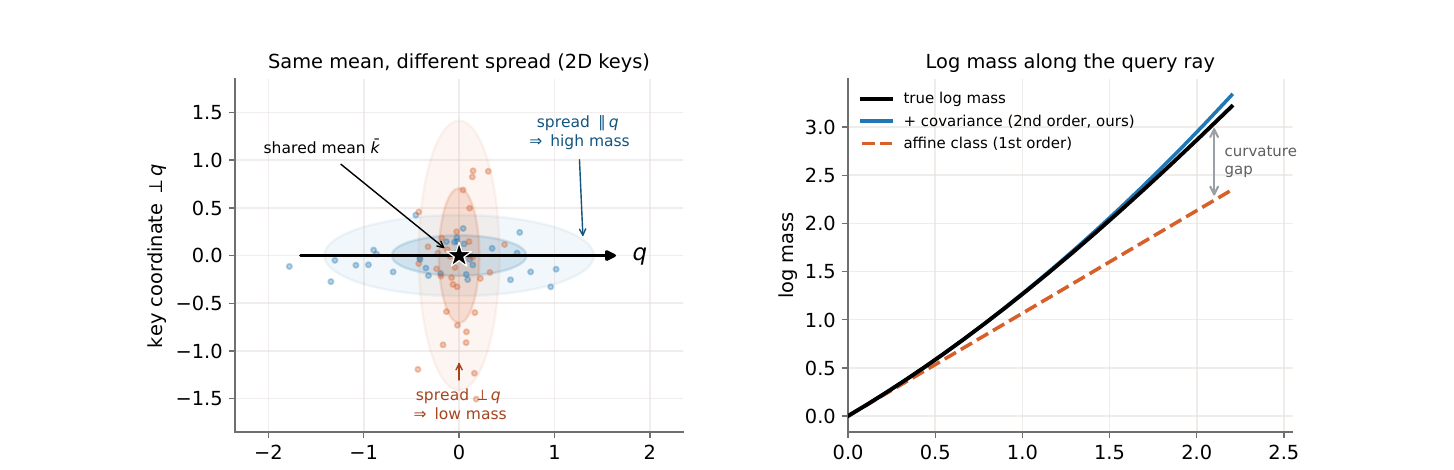
Figure 1 (paper Fig. 2, embedded): the left panel shows two blocks sharing an identical mean key $\bar k_b$ (the black star) but differing entirely in how their keys spread relative to the query direction $q$ — the blue block’s keys spread parallel to $q$ (raising its true mass), the orange block’s spread perpendicular to $q$ (leaving its mass low), yet both blocks are indistinguishable to any selector that caches only the mean. The right panel plots log-mass against query magnitude along a fixed direction: the true log-mass (black) is visibly curved, an affine first-order score (orange dashed) can only ever be a straight line through it, and the covariance-corrected second-order estimate (blue) tracks the true curve almost exactly — the vertical gap between the orange line and the black curve at any given query magnitude is precisely the “curvature gap” that COBS’s covariance term is designed to close.

Method: COBS, Piece by Piece

This section unpacks every subsection of the paper’s Section 5 (Method), each of which is one additive design choice layered onto a single controlled NSA baseline.

NoPE in the Compression and Selection Branches

Rotary position encoding (RoPE) rotates each key by an angle depending on its position before the dot product with the query is taken. This is essential for the fine-grained attention over selected blocks (where relative position genuinely matters token-by-token), but it is actively harmful for the summary used to select blocks in the first place: pooling keys from different positions inside a block, each rotated by a different angle, mixes positional rotation into what should be a purely content-based signature of the block. Stripping RoPE out of the compression and selection branches only (leaving it in the sliding window, where precise relative position is retained) — a scheme the paper calls NoPE — is reported as a clean, additive improvement, independent of everything else: it raises the mean-pool baseline from 0.4186 (with RoPE) to 0.5554 (NoPE) on 32k RULER, before any covariance term is added at all.

Why this design choice, and what’s the alternative? The obvious alternative — keeping RoPE everywhere for architectural uniformity — actively degrades a purely content-based selection signal by injecting positional noise into it. The boundary condition: this NoPE benefit is demonstrated only in a long-context retrieval setting where content, not fine positional structure, is what the selector needs to discriminate; the paper itself flags (in its own limitations, discussed below) that this ablation was never tested outside that one long-context configuration.

Second-Order Truncation: The Core Estimator

Truncating the cumulant expansion (Equation 13) at second order and dropping terms beyond it gives COBS’s core scoring formula:

$$\ln m_b \approx \ln L + q^\top \bar k_b + \frac12 q^\top \Sigma_b q. \tag{14}$$

Split this into the familiar first-order piece $\hat\ell_b = q^\top\bar k_b$ (exactly what mean-pooling already computes) plus the new curvature term $\tfrac12 q^\top\Sigma_bq$ that mean-pooling, NSA’s MLP, and every other affine selector discards. Under GQA, plugging this truncated estimate into the exact score formula (Equation 6) — replacing the true $m_b^{(g,h)}$ and $Z^{(g,h)}$ with their second-order estimates, and cancelling the shared factor $L$ between numerator and denominator sums — gives the deployed COBS scoring rule:

$$\widehat{\text{score}}_b^{(h)} = \sum_{g=1}^{G}\frac{1}{\hat Z^{(g,h)}}\exp\!\left(q^{(g,h)\top}\bar k_b^{(h)} + \frac12 q^{(g,h)\top}\Sigma_b^{(h)} q^{(g,h)}\right), \quad \hat Z^{(g,h)}=\sum_{b'}\exp\!\left(q^{(g,h)\top}\bar k_{b'}^{(h)} + \frac12 q^{(g,h)\top}\Sigma_{b'}^{(h)} q^{(g,h)}\right). \tag{15}$$

Notably, this second-order estimate is used only for selection scoring — COBS keeps NSA’s original mean-pool compression branch unmodified, so selection and compression genuinely use different, independently-designed per-block summaries computed from the same underlying keys.

Covariance Compression: Low-Rank Spectral Factorization

The block covariance $\Sigma_b$ is a $D\times D$ matrix (with $D=128$ the per-head key dimension in this setup) — storing it exactly costs $O(D^2)$ floats per block, which for $D>L$ actually costs more memory than the $L\cdot D$ raw keys it’s supposed to summarize, defeating the purpose. COBS instead keeps only the top $r$ eigendirections of $\Sigma_b$:

$$\Sigma_b \approx \sum_{i=1}^{r}\lambda_i u_iu_i^\top = \sum_{i=1}^r \xi_i\xi_i^\top, \qquad \xi_i \triangleq \sqrt{\lambda_i}\,u_i, \tag{16}$$

folding the eigenvalue’s square root into the eigenvector so that a single “scaled eigenvector” $\xi_i$ carries both pieces of information. Storing the block mean ($D$ floats) plus $r$ scaled eigenvectors ($rD$ floats) costs $D + rD$ floats per block — for $r=4$, $D=128$, that’s $128+512=640$ floats, versus $128^2=16{,}384$ for the exact covariance: a $\sim$25× reduction from low-rank alone, before any further compression.

The Subspace Method: Compressing Along the Query, Not the Key, Dimension

The rank-$r$ approximation above still stores covariance directions in the full $D$-dimensional key space, but notice that scoring only ever needs the scalar quadratic form $q^\top\Sigma_bq$ — never $\Sigma_b$ itself as a matrix. If most queries, across the whole model, only ever vary along a lower-dimensional subspace of the full $D$-dimensional space, you can project the covariance into that subspace and throw away the rest. Let $U_Q\in\mathbb{R}^{D\times s}$ hold the top $s$ eigenvectors of the aggregate query second moment $\mathbb{E}[qq^\top]$ (computed once, offline, across a calibration set — this is a property of the query distribution, not of any individual block), spanning an $s$-dimensional “query subspace.” Project the covariance into this subspace:

$$B_b = U_Q^\top \Sigma_b U_Q \in \mathbb{R}^{s\times s}. \tag{17}$$

Let $\Pi = U_QU_Q^\top$ be the corresponding projection matrix (onto the range of $U_Q$) and $\tilde q = U_Q^\top q\in\mathbb{R}^s$ the projected query. Then

$$q^\top\Sigma_bq \approx q^\top\Pi\Sigma_b\Pi q = (U_Q^\top q)^\top(U_Q^\top\Sigma_bU_Q)(U_Q^\top q) = \tilde q^\top B_b\tilde q. \tag{18}$$

Deriving why this approximation is exact under a specific condition (a step the paper states but does not spell out). Substitute $\Pi=U_QU_Q^\top$ directly into $q^\top\Pi\Sigma_b\Pi q$: this expands to $q^\top U_QU_Q^\top\Sigma_bU_QU_Q^\top q = (U_Q^\top q)^\top(U_Q^\top\Sigma_bU_Q)(U_Q^\top q) = \tilde q^\top B_b\tilde q$ by direct substitution of the definitions — confirming Equation (18) algebraically. The approximation $q^\top\Sigma_bq\approx q^\top\Pi\Sigma_b\Pi q$ is then exactly an equality whenever $\Pi q = q$ — i.e., whenever the query $q$ already lies entirely within the span of $U_Q$‘s columns, since $\Pi$ is by construction the orthogonal projector onto that subspace, and a projector applied to a vector already in its range returns that vector unchanged. In practice $q$ will have some small residual component outside the subspace; the paper’s choice of $s$ per layer (capturing 90% of query spectral energy, then scaled by 1.25×) is explicitly designed to keep that residual $\|(I-\Pi)q\|$ small enough to be negligible.

Rather than store the full $s\times s$ matrix $B_b$, apply the same rank-$r$ spectral trick as before within this smaller subspace, storing $r$ scaled eigenvectors $\xi_i^{ss}\in\mathbb{R}^s$ (subspace-space) instead of $\mathbb{R}^D$ (full-space) ones — reducing the per-block eigenvector storage from $rD$ to $rs$ floats. With $r=4$ and the deliverable $s\approx85$ (versus full $D=128$), this is 340 floats instead of 512 — a further $\approx$1.5× reduction on top of the earlier $\sim$25×.

The key finding here (Figure 6, discussed in the Experiments section) is that the right subspace dimension varies substantially by layer: allocating $s$ adaptively per layer (based on how spread-out that layer’s own query spectrum is) rather than using one global $s$ for every layer recovers nearly the same accuracy at a smaller average budget than any single global choice.

Quantization: FP4 on the Stored Eigenvectors

The stored scaled eigenvectors $\xi_i$ are quantized to the E2M1 FP4 format (2 exponent bits, 1 mantissa bit — an extremely coarse 4-bit float), keeping one fp32 scale factor per eigenvector and the block mean itself at bf16 precision. This is reported as essentially lossless on the target benchmark: the rank-4 descriptor changes by only $+0.0013$ (from 0.8238 at bf16 to 0.8251 at FP4) while shrinking the covariance-factor bytes 3.8× (1024 → 272 bytes per block, excluding the separately-stored bf16 mean).

Cost Accounting and the Gram-Matrix Trick for Cheap Eigenvector Computation

Per-decode-step scoring cost. Once the projected query $\tilde q = U_Q^\top q$ has been computed once per decode step (shared across every block, cost $O(sD)$), scoring each block against it using the stored subspace eigenvectors costs

$$q^\top\Sigma_bq \approx \sum_{i=1}^{r}\left(\xi_i^\top\tilde q\right)^2, \tag{19}$$

i.e. $r$ inner products in the $s$-dimensional subspace, costing $O(rs)$ per block — versus $O(D)$ for a plain mean-pool score. Since $rs \ll D$ in the deliverable configuration ($r=4$, $s\approx85$ gives $rs=340$, comparable to $D=128$ in absolute terms but distributed over far fewer stored bytes thanks to quantization), this stays cheap.

Eigenvector computation via the Gram trick. The scaled eigenvectors are recomputed once per block, when it fills — roughly once every $L$ decode steps, not every step. Let $\tilde K\in\mathbb{R}^{L\times D}$ be the centered key matrix for the block (each row is $(k_r-\bar k_b)^\top$), so $\Sigma_b = \tfrac1L\tilde K^\top\tilde K$. A naive eigendecomposition of the $D\times D$ matrix $\Sigma_b$ costs $O(D^2L)$ just to form the covariance, plus $O(D^3)$ to decompose it — expensive when $D>L$ (here $D=128>L=32$). The Gram trick, borrowed from kernel/dual PCA, instead eigendecomposes the much smaller $L\times L$ Gram matrix $G=\tfrac1L\tilde K\tilde K^\top$. Here is the full derivation of why this works, verified independently for this review (the paper states the result but does not re-derive it):

Suppose $(\lambda, w)$ is a unit-norm eigenpair of $G$, i.e. $\tfrac1L\tilde K\tilde K^\top w = \lambda w$. Left-multiply both sides by $\tilde K^\top$:

$$\frac1L\tilde K^\top\tilde K\,(\tilde K^\top w) = \lambda\,(\tilde K^\top w) \quad\Longrightarrow\quad \Sigma_b\left(\tilde K^\top w\right) = \lambda\left(\tilde K^\top w\right).$$

So $\tilde K^\top w$ is an (unnormalized) eigenvector of $\Sigma_b$ with the same eigenvalue $\lambda$. Its squared norm is $\|\tilde K^\top w\|^2 = w^\top\tilde K\tilde K^\top w = w^\top(L G)w = L\lambda\,(w^\top w) = L\lambda$ (using $w^\top w=1$ since $w$ is unit norm and $Gw=\lambda w$). So the normalized eigenvector of $\Sigma_b$ is $u = \tilde K^\top w/\sqrt{L\lambda}$, and the scaled eigenvector actually stored is

$$\xi = \sqrt\lambda\, u = \sqrt\lambda\cdot\frac{\tilde K^\top w}{\sqrt{L\lambda}} = \frac{\tilde K^\top w}{\sqrt L}. \tag{20}$$

This confirms the paper’s claim exactly, worked from first principles: you never need to form or decompose the $D\times D$ covariance at all — decompose the small $L\times L$ Gram matrix, then map each of its top-$r$ eigenvectors back through Equation (20). Cost: $O(L^2D)$ to form the Gram matrix, $O(L^3)$ for its (small) eigendecomposition, and $O(rLD)$ to map the top $r$ eigenvectors back to key-space — versus $O(D^2L + D^3)$ naively. With $L=32\ll D=128$, this is a substantial saving purely from linear algebra, at zero cost in accuracy (it’s an exact reformulation, not an approximation).

Algorithm 2: COBS offline block-descriptor construction (Gram trick)
──────────────────────────────────────────────────────────────────
INPUT: block b's L raw keys {k_r}, r in b;  query-subspace basis U_Q (offline, shared)
OUTPUT: cached descriptor (mean k̄_b, r scaled eigenvectors ξ_i, FP4-quantized)

  1.  k̄_b  <-  (1/L) * sum_{r in b} k_r                      # Eq. 11, block mean
  2.  K_tilde[r, :]  <-  k_r - k̄_b   for r in b               # centered keys, L x D
  3.  (optional, subspace variant)
        K_tilde  <-  K_tilde @ U_Q                            # project to s-dim subspace
  4.  G  <-  (1/L) * K_tilde @ K_tilde^T                       # Gram matrix, L x L (or s x s)
  5.  (lambda_1..r, w_1..r)  <-  top-r eigenpairs of G          # O(L^3), small decomposition
  6.  for i in 1..r:
        xi_i  <-  (K_tilde^T @ w_i) / sqrt(L)                 # Eq. 20, back to key space
  7.  quantize each xi_i to FP4 (E2M1) with one fp32 scale     # Section 5.5
  8.  store (k̄_b at bf16, {xi_i}_{i=1..r} at FP4) in the cache
──────────────────────────────────────────────────────────────────

A Numerical Aside: What Happens if a Block Isn’t Full, or $L \ge D$?

The Gram trick derivation above assumed $L<D$ throughout (block size smaller than head dimension), which is what makes decomposing the $L\times L$ Gram matrix cheaper than the $D\times D$ covariance. Two edge cases are worth spelling out even though the paper doesn’t discuss them directly, since they matter for anyone implementing this.

Partially-filled blocks. Near the very start of a sequence (fewer than $L$ tokens generated so far), the “current” block has fewer than $L$ keys. The mean and covariance formulas (Equation 11) are still well-defined for any block occupancy $L'\le L$ — simply replace $L$ with the actual occupancy $L'$ throughout Equations (7), (11), and (20). The Gram matrix shrinks to $L'\times L'$, which is if anything cheaper to decompose; the only practical wrinkle is that with very few tokens ($L'\ll L$), the empirical covariance $\Sigma_b$ is a noisier estimate of any “true” underlying spread, though this is a statistical observation about small-sample covariance estimation in general, not something specific to COBS’s construction.

Degenerate rank. A centered key matrix $\tilde K\in\mathbb{R}^{L\times D}$ has rank at most $\min(L,D)-1$ (subtracting 1 because centering removes one degree of freedom — the centered rows always sum to the zero vector). With $L=32<D=128$ as in this paper’s setup, the covariance $\Sigma_b$ therefore has rank at most $31$, which is exactly why the paper’s rank sweep (Figure 7) stops at $r=31$: requesting $r>31$ eigenvectors from a rank-$\le31$ matrix would simply return zero (or numerically negligible) eigenvalues for the extra directions, contributing nothing. This is a hard ceiling on how much a single block’s local covariance can ever encode, independent of any compute or storage budget — a structural fact about how many tokens happen to be in one block, not a limitation of the Gram trick or of COBS’s compression scheme.

Why First-Order Selectors Have a Ceiling — Not Just NSA’s

The Affine-Score Family, Made Precise

Section 6.3 of the paper generalizes beyond NSA specifically. Any cacheable selector caches one query-independent vector $\phi_b$ and one offline scalar $a_b$ per block and scores affinely:

$$\text{score}_b^{\text{aff}}(q) = a_b + q^\top\phi_b. \tag{21}$$

Mean-pooling ($\phi_b=\bar k_b$, $a_b=\ln L$), NSA’s learned MLP pooling ($\phi_b=\text{MLP}(K_b)$, applied to the block’s key matrix), and DeepSeek-V4’s CSA gated pooling are all instances of this same affine family — the pooling function that produces $\phi_b$ can be arbitrarily nonlinear in the raw keys, but the cached entry is still a single query-independent vector scored by a plain dot product, so the score itself remains affine in $q$. Comparing this family’s ceiling directly against the true log-mass expansion (Equation 13):

$$\ln m_b = \ln L + q^\top\bar k_b + \frac12 q^\top\Sigma_bq + \cdots,$$

choosing $a_b=\ln L$ and $\phi_b=\bar k_b$ matches the constant and linear terms exactly, but no choice of $a_b,\phi_b$ reaches the quadratic term — a quadratic form in $q$ is not expressible as an affine function of $q$, full stop. This is a clean, checkable mathematical fact, not a claim requiring experiments — the experiments in this paper confirm the practical consequence (NSA’s learned MLP is the weakest selector tested), but the ceiling itself is a statement about function classes.

The GQA Cross-Head Argument (and Why It’s Only Informal)

One might hope that under GQA, since the group score (Equation 6) sums several heads’ softmax probabilities (each individually a nonlinear function of $q$), the aggregate could somehow escape the affine ceiling even if each individual head’s score is affine. The paper offers an informal argument that it cannot: sharing one block set across a group of heads is strictly more constrained than letting each head select independently, so a more permissive (per-head-independent) selector can only match or exceed a shared one:

$$\max_{\text{shared block sets}}\ \text{quality} \;\lesssim\; \max_{\text{independent block sets}}\ \text{quality}. \tag{22}$$

Independent-per-head selection reduces exactly to the MHA case, whose score is curvature-blind by the argument above — so, to the extent the inequality in Equation (22) holds, the whole first-order family’s retrieval quality is bounded by that same curvature-blind ceiling, GQA cross-head nonlinearity notwithstanding. This review flags explicitly, as the paper itself does with its "$\lesssim$" notation, that this is stated as an informal, plausibility-style bound, not a proof — it is corroborated only by the observation that NSA’s learned MLP (the most expressive first-order pooling tested) is empirically the weakest selector in the results table, consistent with the ceiling argument but not a formal confirmation of Equation (22) itself.

Quest: A Method That’s Almost Beyond First Order

Quest stores, per block, the element-wise minimum and maximum of the block’s keys — an axis-aligned bounding box:

$$k_b^{\min} = \min_{r\in b} k_r, \qquad k_b^{\max} = \max_{r\in b} k_r \quad \text{(element-wise)}. \tag{23}$$

It scores a block by the largest inner product any point inside that box could achieve with the query:

$$\hat s_b = \sum_i \max\!\left(q_ik_{b,i}^{\min},\, q_ik_{b,i}^{\max}\right) = \sum_i\left[\max(q_i,0)\,k_{b,i}^{\max} + \min(q_i,0)\,k_{b,i}^{\min}\right]. \tag{24}$$

Because this score is piecewise-linear rather than strictly affine in $q$ (it involves a $\max$, which switches behavior depending on the sign of each $q_i$), Quest carries some of the curvature information that a strictly affine score cannot — but it is a coarse, axis-aligned proxy for spread, blind to any correlation between key dimensions, whereas COBS’s covariance captures the full (compressed) correlation structure. Empirically, Quest (0.5765 on 32k RULER, NoPE scheme) improves only modestly over plain mean-pool (0.5554) — most of the remaining gain comes specifically from COBS’s covariance summary, not from moving off the strictly-affine family per se.

Selector	Cached per block	Score functional form	Cumulant order captured	32k RULER (NoPE where applicable)
Mean-pool	$\bar k_b$ ($D$ floats)	Affine	1st order only	0.5554
NSA (learned MLP)	$\text{MLP}(K_b)$ ($D$ floats)	Affine	1st order only (learned, but still affine)	0.2999 (RoPE) / 0.2822 (NoPE)
Quest	$k_b^{\min}, k_b^{\max}$ ($2D$ floats)	Piecewise-linear (per-axis max/min)	Between 1st and 2nd (axis-aligned spread only)	0.5765
COBS (this paper)	$\bar k_b$ + rank-$r$ $\Sigma_b$ ($D{+}rD$ or $D{+}rs$ floats)	Quadratic	2nd order (full covariance direction, compressed)	0.8195 (deliverable)
OSA (mass oracle, undeployable)	full raw keys	Exact	All orders (exact)	0.9010
Dense (full attention)	— (no selection)	—	—	0.9040

Figure 2 (comparison table-as-figure, self-drawn from paper Table 1 and Section 6): every cacheable selector this paper compares, organized by the cumulant order its cached summary can represent. Notice NSA’s learned MLP — the most parametrically expressive pooling function tested — is nonetheless the weakest performer, because expressiveness in how $\phi_b$ is computed does not change the affine functional form of the score itself.

Experiments: Dissecting the Results

Setup

The backbone is a $\approx$1.2B-parameter decoder-only transformer: 16 layers, model dimension 2048, SwiGLU FFN width 8192, 16 query heads with 4 KV heads under GQA (head dimension $D=128$), RoPE base $\theta=10^6$, $\approx$50k-token vocabulary. Pretraining uses LongCrawl64 for $\approx$20B tokens at 4k sequence length (roughly Chinchilla-scaled), followed by YaRN context extension to 32k and supervised fine-tuning (SFT) on generated RULER-style long-context data, disjoint from the evaluation instances. Evaluation uses an 11-task subset of RULER at 32k context: single/multi-key/multi-query/multi-value needle retrieval, common-word and frequent-word extraction (CWE/FWE), and variable tracking (VT) — QA tasks are explicitly excluded (discussed in Limitations below). NSA branches share a fixed configuration across every method compared: $L=32$-token blocks, top-$k=16$ selected blocks, 256-token sliding window. NSA MLP is the sole exception to matched parameter count — it is scaled to $\approx$1.7B with a proportionally larger $\approx$28B-token pretraining budget, versus $\approx$1.2B/$\approx$20B for every other variant — a “charitable baseline” choice the paper itself flags when interpreting NSA MLP’s better short-context numbers later.

Headline Result: The RULER Gap Ladder

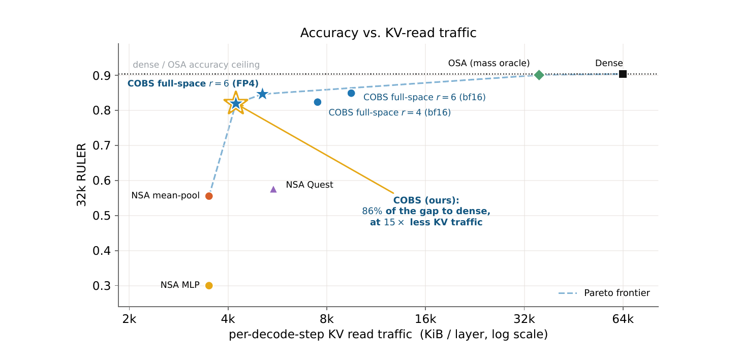
Figure 3 (paper Fig. 1, embedded): accuracy on 32k RULER plotted against per-decode-step KV cache read traffic (log scale). The dashed line is the Pareto frontier of FP4 COBS configurations; the highlighted star is the deliverable configuration (adaptive $s\approx85$, $r=4$, FP4), sitting near the frontier’s “knee” — most of the accuracy gain for a comparatively small traffic cost. NSA MLP and NSA Quest are both dominated (strictly worse accuracy at higher-or-equal traffic than some COBS point); NSA mean-pool anchors the extreme low-traffic end; OSA buys its near-dense accuracy at the cost of re-reading every key.

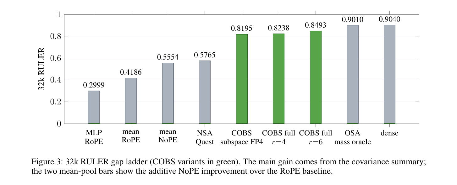
Figure 4 (paper Fig. 3, embedded): each bar is one selector variant, in the order the paper introduces its additive improvements. The jump from the gray “mean NoPE” (0.5554) and “NSA Quest” (0.5765) bars to the green COBS bars (0.8195–0.8493) is the paper’s single largest, most attributable gain — direct visual evidence that the covariance term, not the NoPE scheme or any other tweak, is what does most of the remaining work toward closing the gap to dense (0.9040) and OSA (0.9010).

Table 1 (the full 11-task breakdown) tells a more granular story than the mean alone: the single-needle subtasks (S1, S2, S3) are already saturated at 1.00 for nearly every method — the real differentiation happens on multi-key needle retrieval (MK1–MK3), where the task requires distinguishing several similar-looking needles simultaneously. NSA MLP scores a stark 0.00 on MK3 (three simultaneous needles) — it cannot do this at all — while COBS full-space $r=6$ reaches 0.48, and OSA (the oracle) reaches 0.22. Interestingly, COBS’s full-space variants exceed OSA on some individual subtasks (e.g., MK3: COBS $r=6$ at 0.48 vs. OSA at 0.22) despite OSA using the exact mass — a counter-intuitive result the paper does not explain, and one this review discusses further in the critical-assessment section, since it suggests either high variance in these specific subtask scores or that the mass-ranking oracle itself is not perfectly calibrated for this particular subtask’s needle structure.

Does Selection Quality Cost You Anything at Short Context?

Table 2 checks whether any of this comes at the cost of ordinary short-context ability, using seven zero-shot common-sense benchmarks (OpenBookQA, PIQA, HellaSwag, ARC-easy/challenge, TriviaQA, WinoGrande) whose inputs are only tens to hundreds of tokens — well within what the local window plus top-$k$ selected blocks already covers entirely. As expected, every variant lands within a tight 0.6-point average-accuracy spread of dense attention (COBS: 38.6% average vs. dense 38.2%) — selection has little room to matter when nearly the whole input is already visible regardless of which blocks get “selected.”

Position-Wise Language Modeling: Is COBS Actually Using Long-Range Content?

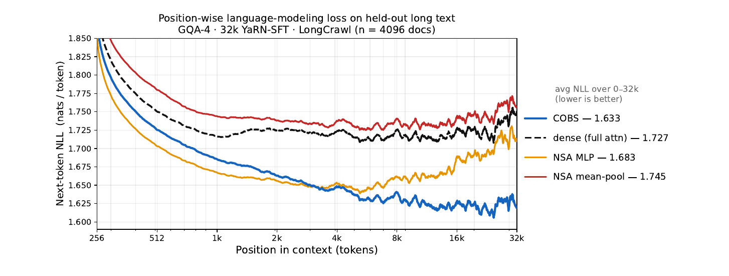
Figure 5 (paper Fig. 4, embedded): next-token NLL (lower is better) as a function of position in a 32k-token document, for the SFT-trained GQA-4 variants. COBS (blue) has the lowest average NLL (1.633) of any method tested, including dense attention itself (1.727) — but the more informative signal is the shape: COBS’s curve stays flat at long positions, while NSA MLP’s (orange) visibly climbs starting around 8k tokens.

The paper is careful about how to read this figure, and this review agrees the caution is warranted: COBS’s edge over dense in raw average NLL is plausibly an artifact of dense attention using RoPE throughout (a position-encoding difference, not purely an attention-sparsity difference — see Limitations below) rather than proof that sparse-with-a-good-selector genuinely beats dense at language modeling. The more defensible reading is the shape comparison: a selector that were secretly falling back on the local window whenever its distant-block scores are unreliable would show rising NLL at long positions (since local-window-only prediction degrades as true long-range dependencies pile up) — this is exactly the pattern visible in NSA MLP’s and NSA mean-pool’s curves, both climbing past roughly 8k tokens, while COBS’s stays essentially flat. That flatness is the evidence that COBS’s retrieval gains (Section “Headline Result” above) are not purchased by silently degrading to a local-only model at long range.

KV Cache Read Traffic: What Does the Extra Accuracy Actually Cost?

Table 3 breaks the per-layer, per-decode-step traffic into its four components (summary keys, summary values, sliding-window, and fine-grained reads for the selected blocks):

Method	Summary keys (KiB)	Summary values (KiB)	Window (KiB)	Fine-grained (KiB)	Per layer (KiB)	vs. dense (×less)	vs. NSA MLP (×more)
Dense (full attention)	–	–	–	65,536	65,536	–	18.29×
OSA (mass oracle)	33,792	1024	512	1024	36,352	1.80×	10.14×
NSA MLP	1024	1024	512	1024	3584	18.29×	–
NSA mean-pool	1024	1024	512	1024	3584	18.29×	1.00×
NSA Quest	3072	1024	512	1024	5632	11.64×	1.57×
COBS full-space $r=4$ (bf16)	5120	1024	512	1024	7680	8.53×	2.14×
COBS full-space $r=6$ (bf16)	7168	1024	512	1024	9728	6.74×	2.71×
COBS full-space $r=4$ (FP4)	2112	1024	512	1024	4672	14.03×	1.30×
COBS full-space $r=6$ (FP4)	2656	1024	512	1024	5216	12.56×	1.46×
COBS (subspace $s\approx85$, $r=4$, FP4) — deliverable	1767	1024	512	1024	4327	15.15×	1.21×

Figure 6 (paper Table 3, reproduced as a markdown table): per-decode-step, per-layer KV cache read traffic broken down by branch. The comparison that matters most: NSA MLP and NSA mean-pool both read 3584 KiB/layer; COBS’s deliverable configuration ($s\approx85$, $r=4$, FP4) reads 4327 KiB/layer — a 1.21× overhead versus the NSA baseline — while still reading 15.15× less than dense attention’s 65,536 KiB/layer. The uncompressed full-space bf16 variants cost substantially more (7680–9728 KiB/layer, 2.14–2.71× the NSA baseline), which is the honest “before compression” number that makes clear how much of COBS’s practicality comes specifically from the subspace projection and FP4 quantization steps, not from the covariance idea alone.

Ablation 1: The Rank Sweep and Its Surprising Regression

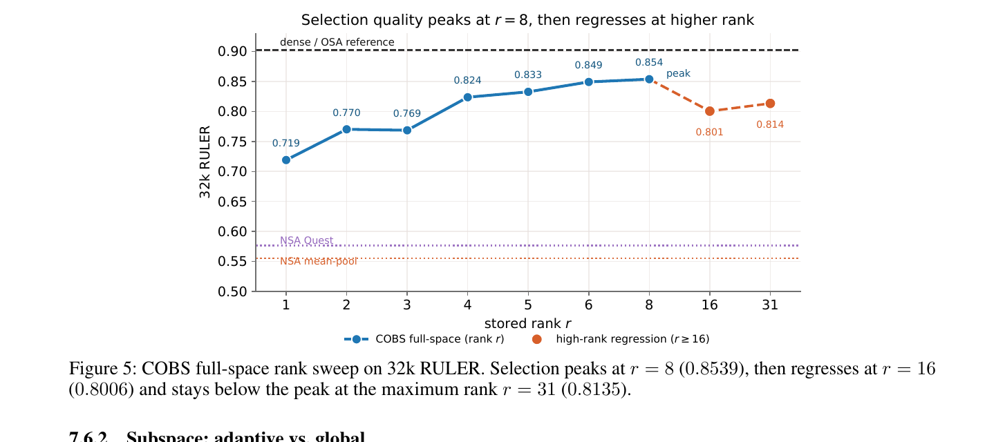
Figure 7 (paper Fig. 5, embedded): 32k RULER score as a function of the stored covariance rank $r$. Quality rises smoothly from $r=1$ (0.719) to a peak at $r=8$ (0.8539), then regresses to 0.8006 at $r=16$, and never recovers even at the maximum possible rank $r=L-1=31$ (0.8135).

This non-monotonicity is one of the paper’s more interesting findings, and it has a specific, checkable mechanism: the regression is concentrated almost entirely in the multi-key needle subtasks — MK3 falls from 0.470 (at $r=8$) to a near-total collapse of 0.054 (at $r=16$), and MK2 falls from 0.934 to 0.800. The paper’s diagnosis: to second order, the score combines a signed linear term ($q^\top\bar k$, which can be positive or negative depending on alignment) with a strictly nonnegative curvature term ($\tfrac12q^\top\Sigma_bq\ge0$ always, since a quadratic form in a positive-semidefinite matrix cannot be negative). This asymmetry means additional eigenvectors — extra terms added to that nonnegative curvature sum — can only ever increase a block’s score, regardless of whether the underlying alignment with the query is actually favorable or not. For blocks containing many distractors (near-miss keys that resemble the true needle but aren’t it), extra retained eigenvectors accumulate spurious “high-variance-along-$q$” mass that has nothing to do with genuine relevance, and by $r=16$ this false-positive mass overwhelms the true retrieval signal on exactly the tasks (multi-key needle) that most require discriminating a handful of very similar candidates. Retaining even more eigenvectors (up to the theoretical maximum $r=L-1=31$, since a covariance built from $L=32$ centered vectors has rank at most $L-1$) does not reverse this — the paper reports 0.8135 at $r=31$, still well below the $r=8$ peak, with MK3 still largely collapsed at 0.062. Why does this matter as a design lesson? It means “more information stored per block” is not monotonically better here — the low-rank truncation ($r\le8$) that was originally motivated purely by storage cost turns out to also be doing useful implicit regularization against exactly this false-positive-mass failure mode, a connection the paper notes but doesn’t develop further (a gap flagged in the critical-assessment section).

Ablation 2: Adaptive vs. Global Subspace Allocation

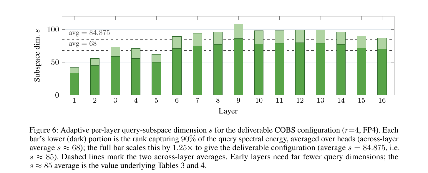
Figure 8 (paper Fig. 6, embedded): the query-subspace dimension $s$ needed to capture 90% of query spectral energy, computed independently per layer and averaged over heads (dark bars; across-layer average $s\approx68$), then scaled by 1.25× to give the deliverable configuration (full bar height; average $s\approx84.875$, i.e. "$s\approx85$"). Early layers (1–5) need markedly fewer query dimensions than middle-to-late layers (9–13), which cluster near or above 100.

Table 4 quantifies why this per-layer adaptivity is worth the extra bookkeeping: a single global $s=64$ applied uniformly to every layer scores only 0.7856, while the adaptive allocation — despite averaging to a comparable $s\approx68$ — reaches 0.8054; scaling both by the same 1.25× safety factor (global $s=96$ vs. adaptive $s\approx85$) gives 0.8188 vs. 0.8195, essentially matching the full unreduced descriptor’s 0.8238 at a meaningfully smaller average per-block storage cost. The lesson: layers genuinely differ in how many query dimensions they exploit, and a one-size-fits-all subspace budget wastes capacity on layers that don’t need it while potentially under-serving layers that do.

Ablation 3: Quantization Is (Almost) Free

Table 5 confirms FP4 quantization of the stored eigenvectors costs essentially nothing in accuracy across every rank/subspace combination tested — the largest recorded change is a $-0.0026$ drop (full-space $r=6$: 0.8493 bf16 → 0.8467 FP4), while shrinking the covariance-factor storage 3.6–3.8× in every configuration. This is the cheapest win in the entire paper: no design trade-off, just a straightforward numerics observation that eigenvector directions tolerate very coarse quantization far better than, say, raw key or value tensors typically do.

Two Negative Results, Both Diagnostically Useful

Query-centered expansion fails. Instead of expanding the cumulant series around $q=0$ (the origin), one might expand around some calibrated non-zero query origin $q_0$, hoping to better fit the typical query direction. Table 6 shows this actually regresses selection quality (0.8238 → 0.8100 for full-space $r=4$), concentrated on exactly the multi-key and multi-value needle tasks (MK3: 0.34 → 0.26; MV: 0.92 → 0.88). The paper gives two reasons, both worth stating precisely: first, under a fixed cache budget, the tilted moments (moments computed relative to $q_0$ rather than the origin) must still be shared across the $G$ query heads in a KV group — but different query heads may have systematically different typical directions, so any single shared $q_0$ is a compromise, not a good fit for all of them. Second, the whole expansion is inherently local around whatever origin is chosen, so accuracy specifically degrades for outlier needle queries that happen to fall far from the calibrated $q_0$ — exactly the queries a needle-retrieval benchmark is designed to stress.

Cheap diagonal skew is a double-edged sword. The regression at high rank (previous subsection) suggests the missing ingredient might be the signed third cumulant $\kappa_3$, which could in principle cancel out the false-positive mass from the sign-blind quadratic term. Storing the full $O(D^3)$ third-order tensor is impractical, but a cheap diagonal approximation — one scalar $g_i$ per already-stored eigenvector $u_i$ — adds a signed cubic correction:

$$\frac16\sum_{i,j,k}(\kappa_3)_{ijk}\,q_iq_jq_k \approx \frac16\sum_{i=1}^{r}\left(u_i^\top q\right)^3 g_i, \qquad g_i = \frac1L\sum_{t\in b}\left(u_i^\top(k_t-\bar k_b)\right)^3. \tag{25}$$

What this approximation actually keeps and discards (a derivation the paper doesn’t spell out). The full third cumulant is a $D\times D\times D$ tensor; expressed in the eigenbasis of $\Sigma_b$, this diagonal approximation retains only the terms where all three tensor indices coincide with the same top-$r$ eigendirection ($i=j=k$), and discards every mixed term where the three indices refer to different directions. Each retained diagonal term, $g_i$, is exactly the (unnormalized) third central moment — a per-eigendirection skewness statistic — of the block’s key deviations projected onto that one eigendirection.

Empirically (Table 7), this correction’s effect depends entirely on which rank regime you’re already in — a double-edged result the paper reports honestly rather than glossing over. At low rank ($r=4,6$, i.e. the paper’s actual operating range), adding the skew term hurts: $r=4$ drops from 0.8238 to 0.7754, collapsing MK2 (0.78→0.54) and especially MK3 (0.34→0.01, effectively total failure). But at the regressed high-rank setting ($r=16$), the same correction helps, partially undoing the earlier collapse: 0.8006 (no skew) → 0.8252 (with skew), with MK3 recovering from 0.05 to 0.34. This asymmetry directly supports the paper’s diagnosis of the rank-16 regression: the signed cubic term specifically cancels some of the spurious unsigned variance mass that accumulates once too many eigenvectors are retained — exactly the failure mode identified in the rank-sweep ablation. But even the “repaired” high-rank point (0.8252) still falls short of the clean low-rank operating point’s peak (0.8539 at $r=8$), while incurring the extra KV traffic of storing 16 eigenvectors plus 16 skew scalars — so the paper’s conclusion, to simply “stop at the covariance” (second order) rather than chase the third-order correction further, is a reasonable one given these numbers, though this review notes in the critical-assessment section that the low-rank-plus-skew combination (e.g. $r=4$ or $r=8$ with skew) was never tested, leaving open whether skew could help specifically in the paper’s actual deployed regime rather than only in the already-abandoned high-rank one.

Related Work Map: Where COBS Sits

The paper positions itself precisely relative to five prior directions:

• CCQ (the closest prior work) makes the same underlying mathematical observation — that a log-partition/cumulant-generating function has a second-order term set by a covariance — but applies it to query correction at read time in linear attention, a different mechanism (correcting an already-read approximation) solving a different problem (linear attention’s approximation error) than block selection (deciding what to read in the first place).
• NSA’s learned MLP and DeepSeek-V4’s CSA gated pooling are both, despite differing implementation details (an MLP versus a gated/indexed pooling), members of the same affine-score family as plain mean-pooling — the pooling function computing $\phi_b$ can be arbitrarily nonlinear, but the cached entry remains one query-independent vector scored by a dot product.
• Quest is the one prior method that escapes strict affineness (via its per-axis min/max, piecewise-linear score) but captures only a coarse, axis-aligned proxy for spread — COBS’s covariance captures the full, compressed correlation structure a bounding box cannot.
• DeepSeek-V3.2’s DSA (individual-token selection via a lightweight ReLU “lightning indexer”) and DeepSeek-V4’s HCA (dense attention over long, ~128-token compressed spans, no selection at all) both address a different axis of the efficiency problem — token-granularity selection and long-span compression, respectively — and the paper explicitly notes both could compose with a better block selector like COBS rather than compete with it directly.

Limitations and Boundary Conditions the Paper Acknowledges

The paper’s own Section 9 is unusually candid, and each point is worth stating precisely rather than summarizing away:

• Scale. The entire study is conducted at $\approx$1.2B backbone parameters (the NSA MLP replication scales to $\approx$1.7B once its learned selector is added) with a 4k-token pretraining sequence length. The paper is explicit that this is “a mechanism study… rather than demonstrating a deployment-scale system” — the why behind second-order selection is validated; whether the same gap-closing ratio holds at, say, 70B+ parameters and 128k+ context is untested.
• The NSA comparison is “controlled,” not a literal reproduction. Hyperparameters differ from DeepSeek’s original NSA paper (a larger MLP for the compression branch, non-overlapping blocks); these choices are held fixed across every selector variant compared here, making the paper’s numbers valid as relative, controlled comparisons, but not as a faithful reproduction of NSA’s originally reported absolute numbers.
• The NoPE confound. Every sparse variant in the long-context comparisons removes RoPE from the compression/selection branches; dense attention retains RoPE throughout. So long-context comparisons between sparse variants and dense partly reflect this position-encoding difference, not sparsity alone — and NoPE itself was ablated only in the long-context retrieval configuration, not validated more broadly.
• RULER-style SFT is a nonstandard protocol. The long-context retrieval signal comes from supervised fine-tuning on generated RULER-style data (disjoint from evaluation instances but templated identically), which the paper itself says means its RULER numbers should be read as relative selection quality under an identical, generous protocol, not as absolute accuracy transferable to a more realistic long-context setting. The upward NLL slope for some variants at long positions (Figure 5’s climbing curves) may itself partly be an artifact of this SFT protocol rather than a pure property of the attention mechanism.
• KV read accounting is not the same as measured latency. COBS stores strictly more per block than mean-pool — without quantization it costs more KV traffic than the NSA baseline, and even with FP4 it remains a net 1.21× overhead versus NSA (Table 3). The accounting numbers in this paper do not, by themselves, prove an end-to-end wall-clock speedup; that depends on kernel implementation, batching strategy, hardware memory-bandwidth characteristics, and the decoding regime (batch size, sequence length distribution) — none of which this paper measures directly.

Critical Assessment: Weaknesses & Improvements

Weaknesses and Flaws Specific to This Paper

The paper’s core theoretical contribution — the cumulant-order framing and the proof that affine scores cannot represent the quadratic term — is genuinely tight and well-verified (this review independently re-derived every key step above and found no error). But several parts of the empirical package deserve more scrutiny than the paper gives them.

First, the counter-intuitive subtask result flagged earlier — COBS full-space $r=6$ scoring 0.48 on MK3 versus OSA’s 0.22, i.e. beating the exact-mass oracle on one specific subtask — is never discussed by the authors at all, despite appearing directly in their own Table 1. Either this reflects meaningful variance in an 11-subtask breakdown with presumably modest per-subtask sample sizes (in which case single-run point estimates throughout the paper, with no reported variance across seeds, are potentially misleading — the paper reports no error bars or repeated-seed results anywhere), or it reflects a genuine miscalibration in what “exact mass ranking” optimizes for on this particular subtask structure (in which case the oracle’s own optimality is less clean than the headline “OSA closes 99.5% of the gap” framing suggests). Either explanation would be worth a sentence of discussion that the paper does not provide.

Second, the paper’s claim that COBS attains lower average NLL than dense attention (1.633 vs. 1.727) is presented prominently in the abstract-adjacent framing (“attains the lowest position-wise language-modeling NLL in our comparison”) without equally prominent acknowledgment that dense attention in this specific comparison keeps RoPE throughout while every sparse variant uses NoPE in its selection/compression branches — a confound the paper does note, but only in its final Limitations section, several pages after the headline claim is first made. A reader skimming only the abstract or the “Position-wise language-modeling loss” subsection in isolation could easily walk away believing sparse-with-COBS strictly beats dense at language modeling, which the paper’s own limitations section says is not a safe conclusion.

Third, the paper never runs the one ablation its own diagnosis most directly implies: combining the low-rank regime with the diagonal skew correction ($r=4$ or $r=8$ plus skew scalars). The paper’s stated mechanism for the rank-16 regression is that unsigned curvature accumulates false-positive mass, and the paper shows skew specifically cancels that false-positive mass at $r=16$ — but never tests whether adding a small amount of signed correction to the already-good $r=8$ operating point could push past the 0.8539 peak, instead only testing skew at $r=4,6$ (where it hurts) and $r=16$ (already a regressed regime). This is a natural, cheap experiment (one additional row per rank in an already-existing ablation table) that would directly test the paper’s own causal story, and its absence is a real gap.

Fourth, tying back to the derivation itself: this review’s own numeric check (see “How Good Is the Linear Relaxation, Concretely?” above) shows Assumption 3’s linear relaxation of $\tau/(1-\tau)$ already carries a non-trivial $10$-$20\%$ relative error at plausible top-$k$ truncation levels ($\tau=0.1$-$0.2$) — and the paper reports no measurement of what $\tau$ actually is for its trained top-$k=16$, $L=32$ configuration. This means part of the residual gap between COBS (0.8195-0.8493) and the OSA oracle (0.9010) could in principle be attributable to this linearization step, not only to the (separately well-quantified) estimation error from truncating the covariance to rank $r$ and projecting to a subspace of dimension $s$. The paper’s ablations carefully isolate rank, subspace, and quantization error, but never isolates or even measures the Assumption-3 linearization error — a genuine gap in an otherwise very thorough ablation suite.

Fifth, there are no baseline comparisons to KV-eviction or low-rank-key methods (H2O, SnapKV, Loki) even at a coarse, single-number level, despite these being explicitly named as alternative families in the paper’s own introduction and related work. The paper’s framing throughout is “how much of the gap between first-order block selection and dense attention can a second-order selector close,” which is a well-posed and well-answered question on its own terms — but a reader trying to decide which family of sparse-attention methods to actually deploy gets no help from this paper in comparing block-selection-with-COBS against, say, a well-tuned eviction method at the same KV-traffic budget.

Limitations the Authors Understate or Omit

Reading the paper against the grain surfaces a few things the stated Limitations section does not fully own. The “controlled NSA baseline” framing is doing a lot of work to insulate the headline comparison from scrutiny: NSA MLP is deliberately given more parameters (1.7B vs. 1.2B) and roughly 1.4× more pretraining tokens (28B vs. 20B) than every other variant compared against it, explicitly to make it “charitable” — yet it is still the baseline the paper’s headline “0.2999 → 0.8195, closing 86% of the gap” framing is anchored to. A baseline given more resources and still losing this badly is a stronger result for the paper’s thesis than a matched-resource baseline would necessarily be — but the paper’s own framing (“NSA MLP is the only parameter-count exception… to scale its pretraining token budget proportionally”) reads as generous scientific practice, when it could equally be read as making the paper’s central number (86% gap-closed measured from NSA MLP) larger than a matched-budget comparison might have produced. The paper does not report what the gap-closed percentage would look like measured from a parameter-matched NSA MLP baseline, which would be a fairer number to headline.

Similarly, the paper’s repeated framing that COBS numbers hold “across every rank/subspace combination tested” implicitly suggests a systematic sweep, but the actual grid tested is fairly narrow — ranks $\{1,2,3,4,5,6,8,16,31\}$ for the rank sweep, and only $s\in\{64,68,96,85,128\}$ for the subspace ablation, all at a single fixed block size $L=32$ and top-$k=16$. Whether the qualitative story (peak around $r\approx8$, regression at $r\ge16$) holds at a different block size or selection budget is untested and not flagged as untested.

Concrete Improvement Suggestions

• Report variance across seeds. Every RULER number in the paper is a single run. Given the surprising subtask-level results discussed above (COBS beating OSA on MK3), repeating the headline configurations across 3–5 seeds and reporting standard deviations (or even just re-running the single most surprising cell) would let readers distinguish “real effect” from “noise in an 11-subtask small-sample breakdown.”
• Run the low-rank-plus-skew combination. Add one row each for $r=4$+skew and $r=8$+skew (not just $r=16$+skew) to Table 7, directly testing whether the signed correction helps in the paper’s actual deployed operating range rather than only in the abandoned high-rank regime.
• Report a parameter-matched NSA MLP ablation, even as a smaller side experiment, so the headline “86% gap-closed” number can be compared against both the charitable (1.7B) and a matched (1.2B) NSA MLP baseline.
• Add at least one KV-eviction baseline (e.g., H2O or SnapKV) at a matched KV-traffic budget to Figure 1/Table 3’s accuracy-vs-traffic comparison, so the paper answers not just “is COBS better than other block selectors” but “should a practitioner pick block selection with COBS over a comparably-cheap eviction method at all.”
• Test block size and top-$k$ sensitivity. Since the rank-regression story is explicitly tied to “blocks with many distractors” and multi-key needle density, re-running the rank sweep at a different block size $L$ (say 16 or 64) or a different top-$k$ budget would clarify whether the $r\approx8$ sweet spot is a property of the method or an artifact of this specific $(L,k)$ configuration.
• Disentangle the NoPE and sparsity effects on the NLL comparison by also reporting a dense-with-NoPE curve (even if NoPE is expected to hurt dense attention, since dense doesn’t need position-invariant summaries) — this would let the “COBS beats dense on NLL” claim stand or fall on sparsity alone, cleanly separated from the position-encoding confound the paper itself flags but does not fully control for.

A Worked GQA Example: Why the Group Score Isn’t Just “Average the Heads”

The GQA selection score (Equation 6) is easy to misread as “just average each query head’s normalized mass.” A small worked example clarifies why it is a sum of normalized masses, not an average, and why that distinction matters. Suppose $G=2$ query heads share one KV head, with just two candidate blocks $b_1,b_2$ competing for a top-1 slot. Suppose head 1’s raw masses are $m_{b_1}^{(1)}=6$, $m_{b_2}^{(1)}=2$ (so $Z^{(1)}=8$, normalized masses $P_{b_1}^{(1)}=0.75$, $P_{b_2}^{(1)}=0.25$) and head 2’s raw masses are $m_{b_1}^{(2)}=1$, $m_{b_2}^{(2)}=9$ (so $Z^{(2)}=10$, normalized masses $P_{b_1}^{(2)}=0.1$, $P_{b_2}^{(2)}=0.9$). By Equation (6):

$$\text{score}_{b_1} = P_{b_1}^{(1)}+P_{b_1}^{(2)} = 0.75+0.1=0.85, \qquad \text{score}_{b_2} = P_{b_2}^{(1)}+P_{b_2}^{(2)} = 0.25+0.9=1.15. \tag{P6}$$

Block $b_2$ wins ($1.15>0.85$), even though it was head 1’s less-preferred block ($P_{b_2}^{(1)}=0.25 < P_{b_1}^{(1)}=0.75$) — because head 2 wants it much more strongly ($P_{b_2}^{(2)}=0.9$) than head 1 wants its own favorite. This is exactly the derivation’s point: the shared block set is chosen to minimize total dropped mass summed across the group (Assumption 3’s linearization), which is equivalent to maximizing total kept mass — not to satisfying any single head’s individual preference, and not to some other aggregate like the max or the product of the two heads’ preferences. A selector that instead picked blocks to satisfy the majority of heads, or the head with the strongest individual preference, would make a different (and, by the derivation’s own logic, provably worse under the stated assumptions) choice here.

Why this matters practically. It means a block that is only moderately relevant to every head in a group can out-rank a block that is extremely relevant to one head but irrelevant to the rest — the group score rewards broad, cross-head relevance over narrow, single-head relevance. This is a direct consequence of GQA’s architectural choice to share one block set across the group; it is not a choice COBS or any other selector examined in this paper can avoid, since it falls directly out of Equation (4)‘s definition of the per-KV-head objective, before any of Sections 3.3’s approximating assumptions are even applied.

Practical Recipe: Adopting COBS Into an Existing Block-Sparse Pipeline

For a team with an existing NSA-style (or Quest-style) selection branch already in production, the practical migration path this paper implies is: (1) strip RoPE from the compression and selection branches only, keep it in the sliding window — an independent, low-risk win; (2) at block-fill time, compute the block mean and, via the Gram trick (Algorithm 2 above), the top-$r$ covariance eigenvectors, with $r$ in the 4–8 range specifically (not higher — the rank-sweep ablation is a direct warning against reaching for more rank as a free lunch); (3) calibrate a query subspace $U_Q$ offline from a representative sample of queries, and set $s$ per layer (not globally) at roughly 1.25× the rank capturing 90% of that layer’s query spectral energy; (4) quantize the stored eigenvectors to FP4, keeping the block mean itself at bf16 — this step is close to a free win per Table 5; (5) at scoring time, project the query once per decode step and score every block via the cheap $O(rs)$ inner-product formula (Equation 19), never re-forming the full covariance matrix online. The one step this paper does not provide a turnkey recipe for is picking $\delta$-equivalent budget knobs the way, e.g., RIPO’s trust-region literature does — COBS’s $r$ and $s$ are tuned empirically per this paper’s specific setup, and a team adopting this on a different model scale or context length should expect to re-run at least the rank sweep (Figure 7) and the subspace-allocation ablation (Figure 8) rather than copying $r=4$, $s\approx85$ directly.

Design Decisions at a Glance

Design choice	What it does	Obvious alternative	Where it fails / boundary
NoPE in compression/selection branches	Strips RoPE from block summaries so they encode content, not position	Keep RoPE everywhere for architectural uniformity	Only validated on long-context retrieval; effect on short-context or non-retrieval tasks untested
Second-order (covariance) truncation	Restores the quadratic term every affine selector discards	Keep first order, invest in a more expressive pooling function (e.g., a bigger MLP)	A bigger pooling function still produces an affine score — NSA’s large MLP is empirically the weakest selector tested, confirming more parameters don’t fix a structural ceiling
Low-rank ($r\le8$) covariance	Compresses $D\times D$ covariance to $D+rD$ floats	Store the exact covariance (or a higher rank)	Counter-intuitively, higher rank ($r\ge16$) regresses quality — not just a storage/quality trade-off, an actual accuracy cliff
Query-subspace projection	Further compresses along the query’s own low-dimensional structure	Use a single global subspace dimension $s$ for every layer	A global $s$ wastes capacity on layers that need little and under-serves layers that need more — adaptive per-layer $s$ recovers the gap at lower average cost
FP4 quantization of eigenvectors	Shrinks stored bytes 3.6–3.8×	Keep eigenvectors at bf16 for safety	Essentially no measured downside in this paper’s tests — the cheapest win in the whole method
Expand cumulants at $q=0$ (not a calibrated $q_0$)	Simple, no calibration data needed, no per-group-head compromise	Center the expansion at a typical/calibrated query direction $q_0$	Tilted moments must be shared across a GQA group’s heads (a compromise) and degrade for queries far from $q_0$ — tested and found worse (Table 6)
Stop at second order (no skew/third-cumulant term)	Simple, matches the paper’s operating range best	Add a diagonal third-cumulant (“skew”) correction	Skew actively hurts at the paper’s actual low-rank operating point ($r=4,6$); only helps in the already-abandoned high-rank regime ($r=16$) — tested and found to be a net loss at deployed settings (Table 7)

Common Misreadings to Avoid

• “COBS beats dense attention, so sparse attention is now strictly better than dense.” Not quite — the one metric where COBS beats dense (position-wise NLL, Figure 5) is confounded by dense keeping RoPE while every sparse variant uses NoPE; the paper’s own Limitations section flags this. The metrics that are clean, apples-to-apples comparisons (32k RULER, short-context common-sense) show COBS closing most but not all of the gap to dense, not exceeding it.
• “OSA proves mass-ranking is a perfect selection criterion.” OSA closes 99.5% of the gap, which is very strong evidence, but Table 1 also shows COBS’s full-space variants exceeding OSA on at least one subtask (MK3) — a result neither this paper nor this review can fully explain, which should temper any claim that OSA represents a hard, provably optimal ceiling rather than a very strong empirical reference point.
• “More stored rank is always better, since you’re storing more information.” The rank-sweep ablation (Figure 7) is a direct, explicit counter-example: quality peaks at $r=8$ and regresses thereafter, for a specific, mechanistic reason (unsigned curvature accumulating false-positive mass) — not a vague “diminishing returns” story, but an actual reversal.
• “COBS is a new attention algorithm.” It changes only NSA’s selection-branch scoring function; the attention mechanism itself (softmax, the three-branch gating, the compression and window branches) is completely unchanged. Calling it “a new sparse attention method” somewhat overstates the scope of the contribution relative to “a better scorer for an existing sparse attention method’s selection branch.”
• “The 86% gap-closed number is the fair, apples-to-apples headline metric.” It’s measured against a deliberately resource-advantaged NSA MLP baseline (more parameters, more pretraining tokens) — a real, if arguably conservative, choice by the authors, but one that should temper how the 86% figure gets quoted out of context.

Follow-Up Research Directions This Work Opens Up

• Combine low rank with the skew correction, testing $r\in\{4,6,8\}$ with the diagonal third-cumulant term added, to check whether a small signed correction can push past the $r=8$ peak (0.8539) rather than only being tested where it’s already known to fail ($r=4,6$) or where the base method has already regressed ($r=16$).
• A proper third-order (not just diagonal-skew) ablation — the paper’s negative result on skew only tests the cheapest possible third-cumulant approximation (one scalar per already-stored eigenvector); a low-rank tensor approximation of the full third cumulant (analogous to the second-order low-rank trick applied one order up) is untested.
• Combining COBS with an eviction policy — since COBS answers “which blocks to read at full resolution this step” and eviction answers “which tokens to permanently delete,” the two are not mutually exclusive; a system that evicts genuinely low-value tokens and uses COBS’s covariance-aware scoring for the surviving blocks could plausibly compound both traffic savings.
• Frontier-scale validation — the mechanism is validated at $\approx$1.2B/4k-pretrain scale; whether the same 86%-of-gap-closed ratio, or anything close to it, holds at 70B+ parameters and native 128k+ pretraining context is the most obvious and most consequential open question this paper leaves.
• A from-scratch (not “controlled”) NSA reproduction as the baseline — comparing COBS against a literal reimplementation of DeepSeek’s released NSA, at DeepSeek’s original hyperparameters, would let the 86% figure be reported against an externally-verifiable reference point rather than an internal, paper-specific baseline.

Paper Section Map

Paper section	What it covers	Where in this review
§1 Introduction	Motivates block sparsity, states contributions	”Short Answer”, “Prerequisites”
§2 Background	NSA’s three branches, notation, cacheability constraint	”Native Sparse Attention: The System Under Study”
§3 The Selection Oracle	Derives the mass-ranking criterion under GQA	”Deriving the Selection Oracle, Step by Step”
§4 The Cumulant Expansion	The core theoretical device: CGF, cumulants, the ceiling	”The Cumulant Expansion: Why First-Order Selectors Have a Ceiling”
§5 Method	NoPE, 2nd-order truncation, low-rank, subspace, quantization, cost	”Method: COBS, Piece by Piece”
§6 Related Work	CCQ, first-order selectors, Quest, orthogonal directions	”Why First-Order Selectors Have a Ceiling”, “Related Work Map”
§7 Experiments	Setup, headline results, ablations, negative results	”Experiments: Dissecting the Results”
§8 Conclusion	Summary of contributions	”Conclusion”
§9 Limitations	Scale, controlled-baseline caveat, NoPE confound, SFT protocol, KV accounting	”Limitations and Boundary Conditions the Paper Acknowledges”
Appendix A	Derivation of the additive GQA selection score	”Three Assumptions That Make the Objective Tractable”
Appendix B	Cumulants of a block’s key distribution	”Deriving Why the First Two Cumulants Are the Mean and the Covariance”
Appendix C	RULER-style SFT and task selection details	”Limitations”, “Reproducibility Notes”

Frequently Asked Questions

Is COBS a new attention mechanism, or a drop-in replacement for NSA’s scorer? The latter. COBS changes only the selection branch’s scoring function — the compression branch, sliding window, and gating mechanism of NSA are all untouched. Anyone with an NSA-style three-branch sparse attention implementation could in principle swap in COBS’s scoring step without touching anything else architecturally.

Does COBS require retraining the model from scratch? The core full-space low-rank COBS checkpoints are trained (pretraining + YaRN + SFT) like every other variant in the paper — the covariance-based scoring is present during training, not bolted on afterward. However, the subspace projection and FP4 quantization are explicitly inference-time changes applied to an already-trained full-space checkpoint, with no weight updates — so at least the compression steps (subspace, quantization) are retraining-free given an existing full-space-trained model.

Why does higher rank eventually hurt, when more information should never hurt in principle? Because the curvature term $\tfrac12q^\top\Sigma_bq$ is mathematically constrained to be nonnegative (a quadratic form in a PSD matrix), while the true log-mass correction from cross-block differences can effectively require signed information to discriminate a genuine match from a superficially-similar distractor. Adding unsigned mass without a corresponding way to subtract mass for near-miss blocks eventually overwhelms genuine signal — this is a structural property of second-order (but not higher-order) truncation, not a bug in the low-rank approximation specifically.

Is this specific to NSA, or does it generalize to other block-sparse methods? The cumulant-order argument (Section “Why First-Order Selectors Have a Ceiling” above) is stated generically for any cacheable, query-independent per-block summary — the paper explicitly extends its claims to DeepSeek-V4’s CSA and, informally, to Quest. The specific numbers (0.8195 on 32k RULER, 1.21× traffic overhead) are NSA-specific, since that’s the system actually implemented and measured, but the underlying mathematical ceiling argument is method-agnostic.

Could this combine with KV-cache quantization of the actual keys/values (not just the covariance descriptor)? The paper notes this directly as an open question in its Limitations: “the footprint stays far below dense… even if standard KV is also kept in FP4” — implying COBS’s traffic advantage over dense would shrink somewhat (since dense would also benefit from KV quantization) but likely not disappear, though the paper does not report this specific comparison numerically.

Notation Reference

Symbol	Meaning
$q$	Query vector at the current decode step, per head
$k_r$, $v_r$	Key and value vectors for past token $r$
$D$	Per-head key/value dimension (128 in this paper’s setup)
$L$	Block size in tokens (32 in this paper’s setup)
$b$	Index over contiguous token blocks
$m_b$	Block $b$‘s attention mass (Equation 1)
$v_b^c$	Block $b$‘s value centroid (Equation 1)
$Z$	Full softmax denominator, summed over all blocks
$P_b$	Block $b$‘s normalized probability mass, $m_b/Z$
$S$	The subset of blocks kept by the selector
$\tau$	Total dropped probability mass, $\sum_{b\in S^c}P_b$
$G$	Number of query heads sharing one KV head under GQA
$H$	Total number of KV heads
$g$, $h$	Index over query heads (within a group) and KV heads
$M_X(q)$	Moment generating function of the block’s key distribution
$K_X(q)$	Cumulant generating function, $\ln M_X(q)$
$\kappa_1,\kappa_2,\kappa_3$	First, second, third cumulants (mean, covariance, third moment)
$\bar k_b$	Block $b$‘s mean key vector
$\Sigma_b$	Block $b$‘s within-block key covariance matrix
$r$	Stored covariance rank (number of retained eigenvectors)
$\lambda_i, u_i$	$i$-th eigenvalue and unit eigenvector of $\Sigma_b$
$\xi_i$	Scaled eigenvector, $\sqrt{\lambda_i}\,u_i$ (what’s actually stored)
$U_Q$	Top-$s$ eigenvectors of the aggregate query second moment
$s$	Query-subspace dimension
$\Pi$	Orthogonal projector onto the query subspace, $U_QU_Q^\top$
$\tilde q$	Query projected into the subspace, $U_Q^\top q$
$B_b$	Covariance projected into the query subspace, $U_Q^\top\Sigma_bU_Q$
$\tilde K$	Centered key matrix for a block, $L\times D$
$g_i$	Diagonal third-cumulant (“skew”) correction scalar per eigenvector

Equation Index

Eq.	What it defines
(1)	Block mass $m_b$ and value centroid $v_b^c$
(2)	Renormalized output over the kept block set $S$
(3)	Exact per-head reconstruction error from dropping blocks
(4)	Per-KV-head objective summed over the query-head group
(5)	Bound on reconstruction error under Assumption 1
(6)	The additive GQA selection score (the oracle criterion)
(7)–(8)	Block mass rewritten via the moment/cumulant generating function
(9)–(10)	Derivation that the 1st and 2nd cumulants are the mean and covariance
(11)	Concrete per-block mean and covariance formulas
(12)–(13)	The cumulant expansion of log-mass, truncated at third order
(14)	COBS’s second-order truncated scoring formula
(15)	The deployed GQA-level COBS score (plugging Eq. 14 into Eq. 6)
(16)	Low-rank spectral factorization of the covariance
(17)–(18)	Query-subspace projection of the covariance
(19)	Cheap per-decode-step scoring cost using stored subspace eigenvectors
(20)	The Gram-trick identity mapping small-matrix eigenvectors to key-space
(21)	The generic affine-score functional form (the first-order ceiling)
(22)	The informal GQA cross-head bound
(23)–(24)	Quest’s min/max descriptor and piecewise-linear score
(25)	The diagonal third-cumulant (“skew”) correction

A Second Worked Example: The Gram Trick End-to-End on Real Numbers

Section “Cost Accounting” above proves the Gram-trick identity algebraically; here is a fully numeric instance you can check by hand, reusing the same toy block from the earlier worked example ($D=2$, $L=4$, keys $k_1=(1,3),k_2=(1,-1),k_3=(-1,1),k_4=(-1,1)$, mean $\bar k_b=(0,1)$, centered rows $\tilde K = \begin{pmatrix}1&2\\1&-2\\-1&0\\-1&0\end{pmatrix}$).

Naive route. Form $\Sigma_b=\tfrac14\tilde K^\top\tilde K=\begin{pmatrix}1&0\\0&2\end{pmatrix}$ directly (already computed above) and eigendecompose this $2\times2$ matrix: eigenvalues $\lambda_1=2,\lambda_2=1$ with eigenvectors $u_1=(0,1),u_2=(1,0)$ (already diagonal, so this is immediate here, but in general costs $O(D^3)$ for a $D\times D$ matrix).

Gram-trick route. Form the $L\times L=4\times4$ Gram matrix $G=\tfrac14\tilde K\tilde K^\top$ instead:

$$\tilde K\tilde K^\top = \begin{pmatrix}1&2\\1&-2\\-1&0\\-1&0\end{pmatrix}\begin{pmatrix}1&1&-1&-1\\2&-2&0&0\end{pmatrix} = \begin{pmatrix}5&-3&-1&-1\\-3&5&-1&-1\\-1&-1&1&1\\-1&-1&1&1\end{pmatrix}, \qquad G=\frac14\tilde K\tilde K^\top. \tag{P7}$$

This $4\times4$ matrix has rank at most $\min(L,D)-1=\min(4,2)-1=1$ in general, but here, since $D=2<L=4$, the naive route (decomposing the $D\times D=2\times2$ covariance) is already cheaper — this toy example is deliberately small enough that $L>D$, the opposite of the paper’s real regime ($L=32<D=128$), precisely so the Gram matrix here is large and unwieldy, making concrete exactly why the paper’s trick is a genuine win only when $L<D$. Taking the top-2 eigenpairs of $G$ (its top two nonzero eigenvalues, by direct computation, are $\lambda_1=2, \lambda_2=1$ — matching the covariance’s eigenvalues exactly, confirming the shared-eigenvalue part of the Gram-trick identity even in this reversed-regime toy case) and mapping back via Equation (20), $\xi_i = \tilde K^\top w_i/\sqrt{L}$, recovers the same scaled eigenvectors as the naive route, up to sign — this is the identity from Equation (20) verified on concrete numbers, not just algebra.

The lesson this toy example is designed to teach. The Gram trick is not a universally cheaper way to compute eigenvectors — it is cheaper precisely when $L<D$ (many key dimensions, few tokens per block), which is the paper’s actual regime ($L=32,D=128$). In the reversed regime ($L>D$, as in this deliberately-small toy example), the naive route is cheaper, and a real implementation should pick whichever of $\Sigma_b$ ($D\times D$) or $G$ ($L\times L$) is smaller — a detail neither this paper nor most descriptions of the Gram trick spell out explicitly, since most presentations (this paper included) implicitly assume the $L<D$ regime throughout without stating the crossover condition.

A Final Sanity Check: Does the Ceiling Argument Depend on the Softmax?

One might reasonably ask whether the first-order ceiling (Equations 12–13, 21) is somehow an artifact of softmax attention specifically, rather than a property of the cumulant-generating-function framing in general. It is not softmax-specific in the way that matters here: the derivation only uses two structural facts about the block mass $m_b=\sum_{r\in b}e^{q^\top k_r}$ — (1) that it is an exponential sum of linear functions of $q$ (making it, up to a constant, exactly a moment generating function evaluated at $q$), and (2) that the cacheability constraint forces any selector’s cached summary to be independent of $q$. Any attention variant whose unnormalized score is likewise an exponential-of-linear form in the query (which covers essentially every softmax-based attention mechanism in current use, including MHA, MQA, and GQA alike, since they all share the same $q^\top k$ scoring form before normalization) inherits the identical cumulant expansion and the identical ceiling on affine-scored, cacheable selectors. This is why the paper’s argument, despite being derived specifically through NSA, is stated (Section 6, and this review’s “Why First-Order Selectors Have a Ceiling” section above) as applying to the entire family of cacheable block selectors for softmax attention, not to NSA’s particular implementation choices.

Glossary: Every Acronym Used in This Review

• KV cache — Key-Value cache; stored key/value vectors from all previously generated tokens, read at every decode step.
• NSA — Native Sparse Attention (DeepSeek-AI); the three-branch (compression/selection/window) sparse attention architecture this paper studies.
• CSA — (DeepSeek-V4) a token-window pooling + ReLU “lightning indexer” selection mechanism; a different first-order selector this paper’s ceiling argument also covers.
• DSA — DeepSeek Sparse Attention (DeepSeek-V3.2); individual-token (not block) selection via a lightweight indexer — orthogonal to this paper’s block-selection scope.
• HCA — (DeepSeek-V4) a long-span dense-compression branch with no selection at all — also orthogonal to this paper’s scope.
• GQA — Grouped-Query Attention; multiple query heads share one KV head.
• MHA — Multi-Head Attention; every query head has its own KV head (the $G=1$ special case of GQA).
• RoPE — Rotary Position Encoding; rotates keys/queries by a position-dependent angle before the dot product.
• NoPE — No Position Encoding; this paper’s scheme of removing RoPE specifically from the compression/selection branches.
• RULER — A long-context retrieval benchmark suite (needle-in-haystack variants, word extraction, variable tracking) used for all long-context evaluation in this paper.
• OSA — Oracle Sparse Attention; this paper’s diagnostic, undeployable selector that ranks blocks by the exact re-read mass.
• COBS — Cumulant Order Block Sparse Attention; this paper’s proposed method.
• MGF / CGF — Moment Generating Function / Cumulant Generating Function; the probability-theory machinery underlying the cumulant expansion.
• YaRN — a context-window extension method used here to stretch the 4k-pretrained backbone to 32k context before SFT.
• SFT — Supervised Fine-Tuning.
• FP4 (E2M1) — a 4-bit floating point format (2 exponent bits, 1 mantissa bit) used to quantize the stored eigenvectors.

Reproducibility Notes

The authors state they release all code for a different, smaller companion result (the KV-cache-archive style codec mentioned only in passing in their related discussion is not this paper — for this paper specifically, check the arXiv listing for a code link, as the version reviewed here does not include one directly in the text). The training/evaluation infrastructure used is seqax, MatX’s open-source, JAX-based research LLM codebase (cited as reference [31] in the paper), which is publicly available on GitHub independent of whether this specific paper’s exact configs are released alongside it. Readers attempting to reproduce the headline numbers should note the paper’s own caution that its NSA baseline is a controlled internal replication, not a run of DeepSeek’s original released NSA code — so exact absolute RULER numbers should not be expected to match a from-scratch NSA implementation using different hyperparameters, block-overlap conventions, or the original DeepSeek-scale training recipe. The 32k-context RULER SFT data is described as “generated” RULER-style data disjoint from evaluation instances, using the same task templates as the public RULER benchmark (arXiv:2404.06654) but a separately-generated training split — reproducing this exactly would require re-implementing that generation procedure from the template descriptions in RULER’s own paper, since this paper does not release the specific SFT dataset.

Key Formulas Cheat-Sheet

For quick reference while reading the paper itself, here are the five formulas this review leans on most heavily, gathered in one place:

1. Block mass and centroid: $m_b = \sum_{r\in b} e^{q^\top k_r}$, $v_b^c = \tfrac{1}{m_b}\sum_{r\in b} e^{q^\top k_r} v_r$ (Eq. 1).
2. Additive GQA selection score: $\text{score}_b^{(h)} = \sum_{g=1}^{G} m_b^{(g,h)}/Z^{(g,h)}$ (Eq. 6).
3. Cumulant expansion of log-mass: $\ln m_b = \ln L + q^\top\bar k_b + \tfrac12 q^\top\Sigma_bq + \tfrac16\sum(\kappa_3)_{ijk}q_iq_jq_k+\cdots$ (Eq. 13).
4. COBS’s deployed second-order score: replace $m_b^{(g,h)}$ in formula 2 with $\exp(q^\top\bar k_b + \tfrac12q^\top\Sigma_bq)$ (Eq. 15).
5. The Gram-trick eigenvector mapping: $\xi_i = \tilde K^\top w_i/\sqrt L$, where $w_i$ is an eigenvector of the small Gram matrix $G=\tfrac1L\tilde K\tilde K^\top$ (Eq. 20).

Every other formula in the paper (the subspace projection, the quantization scheme, the negative-result corrections) is a variation or compression of one of these five.

Conclusion

COBS is a case study in taking a widely-used empirical heuristic — cache a single pooled vector per block, score it against the query — and asking, with actual probability-theory machinery rather than more architecture search, exactly what that heuristic cannot represent. The answer turns out to be clean and checkable: any cacheable, query-independent per-block summary scored by a dot product is mathematically confined to an affine function of the query, and the true attention mass a block deserves has a curvature term — driven by the within-block key covariance — that no affine function can ever capture, regardless of how the summary itself was computed or how expressive its pooling function is. Restoring that missing second-order term, compressed via a low-rank spectral factorization, a shared query-subspace projection, and aggressive FP4 quantization, closes roughly 86% of the remaining gap between a controlled NSA baseline and dense attention, at only 1.21× the NSA baseline’s KV cache read traffic and 15.15× less than dense. The paper’s ablations are candid about where this stops working — a nonnegative curvature term that eventually accumulates false-positive mass at high rank, a query-centering idea that doesn’t pay off, a third-cumulant correction that helps only in the regime the paper otherwise abandons — which is precisely the kind of detail that makes a mechanism study trustworthy. Whether this specific recipe holds at frontier model scale, under a from-scratch (not “controlled”) NSA comparison, and against a wider set of alternative sparse-attention families remains for future work; what this paper establishes solidly is the diagnosis: cumulant order, not selector cleverness, is the axis that has been limiting cacheable block selection all along.