RIPO: Why PPO's Ratio Clipping Is the Wrong Metric, and What Riemannian Geometry Fixes

Review date: 2026-07-14 Review author: Zhongzhu Zhou Paper reviewed: Beyond Euclidean Clipping: Overcoming Exploration Collapse in LLM RL via Riemannian Isometric Policy Optimization Paper authors: Zhicheng Cai, Xinyuan Guo, Hanlin Wu, Mingxuan Wang, Wei-Ying Ma, Ya-Qin Zhang, Hao Zhou arXiv: 2607.10169 Status: ICML 2026 (PMLR 306) — Institute for AI Industry Research (AIR), Tsinghua University & ByteDance Seed

Short Answer

Every popular RL recipe used to post-train LLMs today — PPO, GRPO, DAPO, GSPO, and their many cousins — inherits a single design decision from 2017: clip the importance ratio $r=\pi(a|s)/\pi_{old}(a|s)$ to a fixed interval like $[0.8, 1.2]$, and block gradient flow on anything that falls outside it. This paper’s central claim is that this decision, while cheap and historically successful, silently measures the wrong quantity. The ratio deviation $|r-1|$ is a Euclidean distance on the space of probability ratios — it treats “the ratio moved from 1.0 to 1.2” as the same amount of “policy change” no matter what the starting probability was. But the thing PPO’s clip is supposed to approximate — the trust-region constraint from TRPO — is a bound on KL divergence, and KL divergence induces a Riemannian geometry on the space of policies, one where the same ratio deviation corresponds to wildly different amounts of actual distributional change depending on the token’s starting probability. Concretely: a rare token moving from probability $0.0001$ to $0.01$ has ratio $100$ — deep inside PPO’s clip zone, heavily suppressed — yet moves only about $1\%$ of probability mass. A dominant token moving from $0.99$ down to $0.80$ has ratio $\approx 0.81$ — barely clipped, if at all — yet moves $19\%$ of probability mass, nineteen times more actual distributional shift. PPO’s clip fires on the wrong one, systematically starving rare-but-informative “exploration” tokens of gradient while letting common tokens swing disproportionately, and empirically this is exactly the mechanism behind the well-documented “exploration collapse” failure mode in LLM RL. The paper’s fix, Riemannian Isometric Policy Optimization (RIPO), replaces PPO’s fixed-width clip with a clip boundary that depends on the token’s own old-policy probability, $\epsilon_{s,a}(\pi_{old}) = \sqrt{\delta / \pi_{old}(a|s)}$, chosen so that every clipped update — rare token or dominant token — consumes exactly the same, constant amount of trust-region “budget” $\delta$ on the underlying Riemannian manifold. This single formula change, requiring no new network, no new loss term beyond an adjusted clip boundary, delivers up to 60% relative improvement over GRPO on AIME24 and consistent gains across four model families, seven math benchmarks, and additional coding/search generalization tasks — while also, as a byproduct of the same geometric argument, fixing a heteroscedastic-variance problem in the underlying importance-sampling estimator that made PPO-Clip’s bias-variance trade-off worse than it needed to be.

Key Takeaways

• PPO-Clip’s ratio-deviation constraint $|r-1|\le\epsilon$ implicitly assumes a Euclidean metric on policy space: any two token updates with the same ratio deviation are treated as equally “large” changes, regardless of the token’s starting probability.
• The actual discrepancy between two policies is governed by KL divergence, whose second-order Taylor expansion is a quadratic form in the Fisher Information Matrix — this induces a Riemannian manifold on the space of policies, where distances in high-probability regions are geometrically “stretched” relative to distances in low-probability regions.
• Working through the algebra (Eq. 4–8 in the paper), the true geometric distance moved by a single-token update turns out to be $d_{geom}\propto \pi_{old}(a|s)\cdot(r-1)^2$ — proportional to the old probability, not just the ratio deviation. This is the one-line reason PPO’s fixed clip is miscalibrated: it is blind to the $\pi_{old}$ factor entirely.
• Riemannian Isometric Clip (RIC) solves for the ratio bound that keeps $d_{geom}$ constant across all tokens: $\epsilon_{s,a}(\pi_{old})=\sqrt{\delta/\pi_{old}(a|s)}$ — a clip boundary that widens for rare tokens and narrows for dominant tokens, in contrast to PPO/DAPO’s single fixed number for every token in the vocabulary.
• On the numeric worked example in the paper: with $\delta=0.02$, a token at $\pi_{old}=0.8$ is now capped at probability $0.92$ (tighter than PPO’s $0.96$), while a token at $\pi_{old}=0.01$ is allowed up to $0.024$ (nearly double PPO’s $0.012$) — both updates consume the same $0.01$ of geometric trust-region budget, versus PPO’s wildly uneven $0.016$ vs. $0.0002$.
• Beyond fixing the clip boundary, the paper shows RIC also improves the bias–variance trade-off of the underlying importance-sampling estimator: because the clip threshold now scales as $1/\sqrt{\pi_{old}}$, the variance contribution of every clipped sample becomes $O(\delta)$ — constant, density-independent — a property called statistical homoscedasticity, versus PPO-Clip’s heteroscedastic (probability-dependent) variance.
• RIPO plugs RIC directly into the GRPO objective (replacing GRPO’s fixed $\epsilon$ with the dynamic $\epsilon_{s,a}(\pi_{old})$), keeping every other part of the training recipe — group-relative advantage, token-level loss aggregation — completely unchanged.
• Across four base models (Qwen3-1.7B/4B/8B-Base, Llama3.2-3B-Instruct) and seven competition-level math benchmarks, RIPO beats GRPO by 37.2%, 34.4%, 17.1%, and 35.1% (relative, on average), and consistently beats four more sophisticated GRPO variants (DAPO, GSPO, GMPO, DCPO) on the harder benchmarks (AIME24, BRUMO25).
• Training dynamics diagnostics (Fig. 1) show RIPO reaching GRPO’s 200-step performance in only 40 steps (5x token-efficiency), maintaining moderate, non-collapsing policy entropy (unlike GRPO’s entropy collapse or DAPO’s entropy explosion), and an almost fluctuation-free gradient norm throughout training.
• A δ-ablation (Table 2) shows RIPO is robust to its one new hyperparameter across a broad range ($\delta\in[0.02,0.08]$), but breaks down sharply if the lower and upper δ budgets are made highly asymmetric — reward degrades suddenly with an entropy explosion, confirming that both directions of the clip must be geometrically constrained together.
• RIPO’s clip mechanism (RIC) transfers cleanly beyond GRPO: applied to the vanilla PPO objective with a learned critic on GSM8K, RIPO-Clip still beats PPO-Clip, DAPO-Clip, and DCPO-Clip at every model scale from 0.5B to 14B — evidence that the fix is about the clip’s geometry, not anything specific to GRPO’s advantage estimator.
• Generalization checks on long-horizon coding (Codeforces, CodeContest, TACO, APPS) and multi-hop search (TriviaQA, PopQA, HotpotQA, WikiMultiHopQA) both show RIPO extending its advantage over GRPO beyond math reasoning, suggesting the geometric mismatch this paper identifies is a property of long-tailed token distributions generally, not an artifact of one task family.

Prerequisites: What You Need to Know First

This paper sits at the intersection of three things you need in place before the core argument makes sense: (1) the classical trust-region policy optimization story (TRPO → PPO → GRPO), (2) enough differential-geometry vocabulary to understand what a “Riemannian manifold” and an “isometric” update mean in this context, and (3) the specific empirical phenomenon of “exploration collapse” in LLM RL that motivates the whole paper. I build these up in order below; if you already know the PPO/GRPO story well, skip to “The Riemannian Geometry Lesson,” which is the part that is genuinely new relative to standard RL-for-LLM background.

From MDPs to Trust Regions: The Classical Story

A Markov Decision Process is the tuple $(\mathcal{S},\mathcal{A},P,r,\rho_0,\gamma)$: state space, action space, transition dynamics, reward function, initial-state distribution, and discount factor. A policy $\pi(a|s)$ generates trajectories by sampling actions and following the transition dynamics; the RL objective is to maximize expected discounted return. The advantage function $A^\pi(s,a)=Q^\pi(s,a)-V^\pi(s)$ measures how much better action $a$ is than the policy’s average behavior at state $s$: positive means “reinforce this,” negative means “suppress this.”

Trust Region Policy Optimization (TRPO), Schulman et al. (2015), proves that if you maximize an importance-weighted surrogate objective $L_{\pi_{old}}(\pi)=\mathbb{E}_{s\sim\rho_{old},a\sim\pi_{old}}\left[\frac{\pi(a|s)}{\pi_{old}(a|s)}A^{\pi_{old}}(s,a)\right]$ subject to a hard constraint that the KL divergence between old and new policy stays below some threshold $\delta$, you get a monotonic-improvement guarantee: the true return $\eta(\pi)$ never decreases. This constrained problem,

$$\max_\pi\ L_{\pi_{old}}(\pi)\quad\text{s.t.}\quad \mathbb{E}_{s\sim\rho_{old}}\big[D_{KL}(\pi_{old}(\cdot|s)\,\|\,\pi(\cdot|s))\big]\le\delta, \tag{1}$$

is what “trust region” formally means: a hard divergence budget, not a soft heuristic. But solving Equation 1 exactly requires a second-order (natural-gradient) optimization step, which is expensive and hard to scale to billion-parameter networks.

Proximal Policy Optimization (PPO), Schulman et al. (2017), replaces this expensive constrained optimization with something far cheaper: directly clip the importance ratio itself,

$$J_{PPO}(\theta) = \mathbb{E}\left[\min\big(r(\theta)\hat{A},\ \operatorname{clip}(r(\theta), 1-\epsilon, 1+\epsilon)\,\hat{A}\big)\right], \tag{2}$$

where $r(\theta)=\pi_\theta(a|s)/\pi_{\theta_{old}}(a|s)$ is the probability ratio and $\epsilon$ (usually $0.2$) is a single, fixed clipping width applied identically to every action in every state. The intuition sold at the time was: if the ratio doesn’t move too far from 1, the policy hasn’t changed too much, so this is a cheap proxy for the KL constraint in Equation 1. This paper’s whole argument is that this intuition — “ratio deviation is a good proxy for KL divergence” — quietly stopped being true once RL was applied to LLMs with 100k+-token, long-tailed vocabularies, even though it was a reasonable approximation in the small, often near-uniform action spaces (Atari, MuJoCo) PPO was originally validated on.

GRPO: Removing the Critic for LLM Fine-Tuning

Training a full value network $V^\pi(s)$ for an LLM is expensive and often noisy given sparse, sequence-level rewards. Group Relative Policy Optimization (GRPO) (Shao et al., 2024; Guo et al., 2025 / DeepSeek-R1) sidesteps this: for a given prompt $q$, sample a group of $G$ responses $\{o_i\}_{i=1}^G$, score each with reward $R_i$, and compute a group-normalized advantage,

$$\hat{A}_{i,t} = \frac{R_i - \operatorname{mean}(\{R_j\}_{j=1}^G)}{\operatorname{std}(\{R_j\}_{j=1}^G)}, \tag{3}$$

then optimize the same PPO-Clip objective (Equation 2) token-by-token, with $r_{i,t}(\theta)=\pi_\theta(o_{i,t}|q,o_{i,<t})/\pi_{\theta_{old}}(o_{i,t}|q,o_{i,<t})$. GRPO keeps PPO’s clip mechanism entirely intact — it only changes how the advantage is estimated, not how the trust region is enforced. This matters for the current paper because it means RIPO’s fix (which targets the clip, not the advantage estimator) is orthogonal to and compatible with GRPO’s advantage estimator — the paper builds RIPO directly on top of GRPO’s advantage formula, changing only the clip boundary.

Concrete numeric example of Equation 3. Suppose $G=4$ responses to a math problem get rewards $R=(1,0,1,0)$ (two correct, two incorrect, binary verifiable reward). The mean is $0.5$; suppose the std is $0.577$ (population std of two 1s and two 0s). Then $\hat{A}=(0.87,-0.87,0.87,-0.87)$. Notice every token inside a correct response gets the identical advantage $+0.87$, whether it was the crucial insight step or a generic connective word — GRPO’s advantage is coarse at the token level. This is exactly why the masking mechanism applied on top of $\hat{A}$ (PPO’s ratio clip, or RIPO’s geometric clip) carries so much of the burden of deciding which tokens actually get to learn efficiently: since the advantage signal itself cannot discriminate within a response, the clip is the only remaining lever.

A Brief History: From Ratio-Clip Patches to Geometric Redesign

• 2015 — TRPO: proves the KL-constrained trust-region template (Equation 1) for classical, typically small- or moderate-cardinality action spaces.
• 2017 — PPO: replaces TRPO’s expensive constrained optimization with cheap ratio clipping (Equation 2) — a reasonable approximation in the small-action-space regime PPO was validated on.
• 2024 — GRPO: adopts PPO’s clip essentially unchanged, now applied over 100k+-token LLM vocabularies, without re-validating whether ratio-deviation is still a good KL proxy at that scale.
• 2025 — symptom patches appear: DAPO’s Clip-Higher widens the upper clip bound ($\epsilon_{high}=0.28>\epsilon_{low}=0.2$) to let more “exploration” tokens through; GSPO and GMPO move to sequence-level or geometric-mean ratio clipping to reduce gradient variance; DCPO adapts clip thresholds dynamically but heuristically; CISPO and GPPO try preserving gradient signal on clipped tokens rather than truncating it. All of these treat the symptom (rare tokens get clipped too hard) without diagnosing why the ratio itself is a bad KL proxy.
• 2026 — this paper: derives, from first principles, exactly what geometric quantity the ratio-deviation clip should have been measuring all along (Riemannian distance under the KL-induced metric), shows the mismatch analytically (Eq. 3–8), and replaces the mispriced quantity rather than patching around its symptoms.

Read this way, RIPO’s contribution is less “yet another clip variant” and more “someone went back and checked whether the load-bearing geometric assumption behind PPO’s clip actually holds at LLM vocabulary scale — and found that it structurally does not.”

The Five Baselines, Formula by Formula

Because the experimental section compares RIPO against five distinct prior clipping mechanisms, it is worth having each one’s actual mathematical definition in view before reading the results, rather than treating them as black-box acronyms. All five share the same GRPO scaffold (group-relative advantage, Equation 3) and differ only in how they compute the clip bound or which quantity they clip.

DAPO (Clip-Higher). Keeps PPO’s ratio-based clip structure exactly, but decouples the lower and upper bounds:

$$\operatorname{clip}_{DAPO}(r,\epsilon_{low},\epsilon_{high}) = \operatorname{clip}(r,\ 1-\epsilon_{low},\ 1+\epsilon_{high}),\quad \epsilon_{high}=0.28 > \epsilon_{low}=0.2. \tag{B1}$$

The design intuition: since PPO’s symmetric clip disproportionately suppresses ratio increases on low-probability tokens (recall the worked example: a rare token’s ratio easily blows past $1.2$), simply allow ratios to rise further before clipping kicks in on the upper side. Why this is a heuristic, not a fix: Equation B1 still uses a single, $\pi_{old}$-independent bound for every token in the vocabulary — it just moves the bound. A token with $\pi_{old}=0.01$ whose ratio spikes to $100$ is exactly as clipped under DAPO’s $\epsilon_{high}=0.28$ as under PPO’s $\epsilon=0.2$, because $100$ is far outside either bound. DAPO only helps the marginal tokens whose ratio happens to land between $1.2$ and $1.28$ — a narrow band that does little for the extreme long tail this paper’s diagnosis is actually about.

GSPO (sequence-level clipping). Instead of clipping each token’s ratio individually, GSPO computes a single ratio for the entire sequence (geometric mean of per-token ratios) and applies the clip once at the sequence level:

$$r_{seq}(\theta) = \left(\prod_{t=1}^{|o|}\frac{\pi_\theta(o_t|q,o_{<t})}{\pi_{\theta_{old}}(o_t|q,o_{<t})}\right)^{1/|o|},\qquad \operatorname{clip}(r_{seq}(\theta),\,1-\epsilon,\,1+\epsilon). \tag{B2}$$

The design intuition: token-level ratios are individually noisy (a single unlucky rare token can trigger a clip that discards gradient for an otherwise-good sequence); averaging in log-space before clipping smooths out this per-token noise. Why this is an incomplete fix from RIPO’s perspective: GSPO changes what is being clipped (sequence vs. token) but not the metric used to decide the clip boundary — it is still an unweighted average of ratios, with no $\pi_{old}$-dependence built in. It reduces token-level noise but does not address the geometric mismatch (Equation 8) at all; a sequence full of rare, informative tokens can still have its aggregate ratio miscalibrated in exactly the Euclidean sense this paper critiques.

GMPO (geometric-mean ratio clipping). Similar in spirit to GSPO but applies the geometric-mean aggregation within the clip’s argument rather than clipping a pre-aggregated sequence ratio, intended to reduce gradient variance from individual extreme-ratio tokens. Shared limitation: like GSPO, this changes the aggregation/smoothing strategy, not the underlying per-token metric — it is a variance-reduction technique layered on top of the same Euclidean assumption RIPO targets.

DCPO (dynamic-adaptive clipping). Adapts the clip threshold based on some measure of training dynamics (e.g., recent statistics of the ratio distribution), rather than using a single constant across the whole training run. Why this is closer to RIPO in spirit but still different: DCPO’s adaptivity is typically a function of training progress or aggregate statistics (a global, time-varying adjustment), not a function of the individual token’s own $\pi_{old}(a|s)$ computed fresh at every single update the way RIC is (Equation 10). DCPO can adjust “the clip should be looser today than last week” but does not have a principled per-token answer to “the clip should be different for this rare token than for that common token, right now, in this same batch” — which is exactly the distinction Table 1 and Table 3’s per-benchmark RIPO margins are evidence for.

GPPO and Clip-Cov (Table 3 comparison set). GPPO preserves the gradient of clipped tokens instead of zeroing it out entirely (addressing information loss from clipping, a different concern from calibration). Clip-Cov clips tokens by their covariance with the advantage rather than by ratio magnitude (addressing entropy regulation directly, rather than trust-region calibration). Both are answers to related-but-distinct questions from the one RIPO asks; Table 3’s results (reproduced in the Experiments section below) show both underperforming RIPO by a wide margin on every benchmark, which the paper reads as evidence that a correctly-calibrated trust region (RIPO’s approach) captures most of the benefit that information-preservation (GPPO) and entropy-regulation (Clip-Cov) partially and separately chase.

Method	What changes vs. PPO-Clip	Is the clip threshold $\pi_{old}$-dependent per token?
PPO / GRPO	baseline	no (constant $\epsilon$)
DAPO	asymmetric constants $\epsilon_{low}\ne\epsilon_{high}$	no
GSPO	sequence-level aggregation before clipping	no
GMPO	geometric-mean ratio inside the clip	no
DCPO	threshold adapts over training time / batch statistics	no (adapts globally, not per-token)
GPPO	preserves gradient on clipped tokens	no
Clip-Cov	clips by advantage-covariance, not ratio	no (different criterion entirely)
RIPO (RIC)	**threshold is $\sqrt{\delta/\pi_{old}(a	s)}$, recomputed per token**

Figure 4b (design-choice comparison, table-as-figure): of eight methods sharing the same GRPO/PPO scaffold, RIPO is the only one whose clip threshold is a genuine per-token function of that token’s own old-policy probability — every other method’s adjustment is either a global constant, a global schedule, or an aggregation strategy applied on top of an otherwise still-flat threshold.

The Riemannian Geometry Lesson: What “Isometric” Actually Means Here

This is the part of the background that is genuinely non-standard for most LLM-RL readers, so it is worth building carefully rather than waving at “differential geometry” and moving on.

Step 1 — A metric is just a rule for measuring distance. The Euclidean metric on $\mathbb{R}^n$ says the distance between two points is $\|x-y\|$. But not every space that matters for optimization has a “natural” Euclidean structure. The space of probability distributions over a vocabulary — call it the statistical manifold — does not: two distributions that are “close” in raw parameter difference can produce wildly different behavior, and two distributions “far” in parameter space can behave almost identically. You need a distance measure that respects how the distributions actually behave, not how their raw numbers differ.

Step 2 — KL divergence supplies exactly this behavioral distance, locally. For nearby policies $\pi_{old}$ and $\pi=\pi_{old}+\Delta$, a second-order Taylor expansion of the KL divergence gives

$$D_{KL}(\pi_{old}\|\pi) \approx \frac{1}{2}\Delta\theta^\top F(\theta)\Delta\theta, \tag{4}$$

where $F(\theta)$ is the Fisher Information Matrix. This is precisely the definition of a Riemannian metric: a position-dependent quadratic form that tells you how to measure squared-distance for a small step $\Delta\theta$ at that particular point in parameter space. Unlike the Euclidean metric (a constant identity matrix everywhere), $F(\theta)$ changes as you move around the space — this is what makes the geometry “Riemannian” rather than “Euclidean,” and it is the entire reason this paper’s argument has teeth: the correct notion of “how far did the policy move” depends on where you started, not just on the raw magnitude of the parameter change.

Step 3 — mapping this to per-token probability space. Deriving through the chain rule (Equation 5–7 in the paper; worked step-by-step in the “Theory” section below), the local KL divergence for a single state-action pair reduces to

$$D_{KL}(\pi_{old}(\cdot|s)\|\pi(\cdot|s)) \approx \frac{1}{2}\sum_a \pi_{old}(a|s)\,(r_{s,a}-1)^2, \tag{5}$$

where $r_{s,a}=\pi(a|s)/\pi_{old}(a|s)$. Look closely at the right-hand side: it is not simply “sum of squared ratio deviations” — every term is weighted by $\pi_{old}(a|s)$, the old-policy’s own probability of that action. This weighting is the Riemannian metric made concrete: it says the geometric “cost” of a given ratio deviation shrinks in low-probability regions and grows in high-probability regions. Equation 5 is the single most important formula in this paper’s background, because everything else — the diagnosis of PPO’s flaw and the design of RIPO’s fix — is a direct consequence of this one weighting factor.

Step 4 — “isometric” means equal geometric distance, not equal ratio deviation. An isometry is a transformation that preserves distances measured by the correct metric. RIPO is called “isometric” because its clipping rule is derived to guarantee that every single-token update consumes exactly the same amount of Riemannian distance $d_{geom}=\delta$ (Equation 5’s right-hand side, per-token), regardless of whether that token started at probability $0.0001$ or $0.99$. PPO’s clip, by contrast, guarantees equal ratio deviation ($|r-1|\le\epsilon$) — which, per Equation 5, corresponds to wildly unequal geometric distances depending on $\pi_{old}$. This is the precise, technical content behind the paper’s title: “beyond Euclidean clipping” means moving from a metric that is blind to $\pi_{old}$ (Euclidean) to one that is not (Riemannian), and “isometric” means the clip is redesigned so that its effect is uniform under the correct metric instead of the wrong one.

flowchart TB
    subgraph EUC["Euclidean view (PPO-Clip's implicit assumption)"]
        E1["distance(pi_old, pi) := (r - 1)^2"]
        E2["Same ratio deviation implies same policy change, for ANY pi_old"]
        E1 --> E2
    end
    subgraph RIEM["Riemannian view (this paper's derivation)"]
        R1["distance(pi_old, pi) := pi_old * (r - 1)^2  (Eq. 5)"]
        R2["Same ratio deviation implies DIFFERENT policy change depending on pi_old"]
        R1 --> R2
    end
    EUC -.->|"PPO-Clip enforces equal |r-1| for every token"| MISMATCH["Geometric mismatch:\nrare tokens under-updated,\ndominant tokens over-updated"]
    RIEM -.->|"RIC enforces equal pi_old*(r-1)^2 for every token"| FIX["Isometric fix:\nclip boundary widens for rare tokens,\nnarrows for dominant tokens"]

Figure 1 (architecture / concept overview): the core conceptual shift from Euclidean to Riemannian distance. PPO-Clip’s single fixed $\epsilon$ implicitly assumes the Euclidean view (top); RIPO’s dynamic $\epsilon_{s,a}(\pi_{old})$ is derived directly from the Riemannian view (bottom).

A Fully Worked Numeric Example of the Fisher Information Matrix Step

The algebra in Equations 4–8 is easiest to trust if you can see it work on a small, concrete example rather than only in the abstract. Consider a toy vocabulary of just three tokens, $\{a_1,a_2,a_3\}$, at a single state $s$, with old policy $\pi_{old}(s)=(0.7,\,0.2,\,0.1)$ and new policy $\pi(s)=(0.6,\,0.25,\,0.15)$ (a small, plausible single-step change).

Step 1 — compute the exact KL divergence directly, as a ground truth to check the approximation against: $D_{KL}(\pi_{old}\|\pi)=\sum_a \pi_{old}(a)\log\frac{\pi_{old}(a)}{\pi(a)} = 0.7\log\frac{0.7}{0.6}+0.2\log\frac{0.2}{0.25}+0.1\log\frac{0.1}{0.15}$. Computing each term: $0.7\log(1.1\overline{6})\approx0.7\times0.1542=0.1080$; $0.2\log(0.8)\approx0.2\times(-0.2231)=-0.0446$; $0.1\log(0.6\overline{6})\approx0.1\times(-0.4055)=-0.0405$. Sum: $D_{KL}\approx0.1080-0.0446-0.0405=0.0228$.

Step 2 — compute the second-order (Equation 5) approximation using the same numbers: $\frac{1}{2}\sum_a\pi_{old}(a)(r_a-1)^2$ where $r_a=\pi(a)/\pi_{old}(a)$. Ratios: $r_1=0.6/0.7\approx0.857$, $r_2=0.25/0.2=1.25$, $r_3=0.15/0.1=1.5$. Terms: $0.7\times(0.857-1)^2=0.7\times0.0204=0.01429$; $0.2\times(1.25-1)^2=0.2\times0.0625=0.0125$; $0.1\times(1.5-1)^2=0.1\times0.25=0.025$. Sum $=0.01429+0.0125+0.025=0.05179$; half of that is $D_{KL}^{approx}\approx0.0259$.

Step 3 — compare. Exact $D_{KL}\approx0.0228$ vs. approximation $\approx0.0259$ — a relative error of about $14\%$ for a change this size (some tokens moved by $10$-$17\%$ relative probability, a moderately large single step). This directly illustrates the earlier limitation note: the second-order approximation is accurate for small policy changes (as used throughout classical trust-region theory and as is typical for the tiny, $10^{-6}$-learning-rate updates in LLM RL) but visibly starts to drift for changes of this more noticeable size — a useful concrete sense of how “local” the local approximation really is.

Step 4 — read off the per-token geometric distances (Equation 8) for this example, which is what RIC would actually use for each token individually rather than the state-level sum: $d_{geom}(a_1)=0.5\times0.7\times(0.857-1)^2\approx0.00714$; $d_{geom}(a_2)=0.5\times0.2\times(1.25-1)^2=0.00625$; $d_{geom}(a_3)=0.5\times0.1\times(1.5-1)^2=0.0125$. Notice token $a_3$ — despite having the smallest old probability ($0.1$) among the three — has the largest geometric distance in this particular example, because its ratio moved the most ($1.5\times$). This is an important nuance: RIC’s formula does not simply say “rare tokens always get bigger allowances” in some blanket sense — it says the allowance (the clip width $\epsilon_{s,a}$) scales up for rare tokens, but the actual distance consumed by any specific observed update still depends on how far that update actually moved the ratio, exactly as Equation 8’s product structure implies.

A Note on “Riemannian” as Marketing vs. Mechanism

It is worth being precise about how much actual differential geometry this paper uses, because the word “Riemannian” can oversell the machinery involved. The paper does not use geodesics, parallel transport, curvature tensors, or any of the heavier apparatus of full Riemannian geometry — those would be needed if you wanted to reason about finite, large policy updates along curved paths on the manifold. What it uses is the local, second-order (quadratic) approximation to KL divergence (Equation 4), i.e., the Fisher Information Matrix as a local Riemannian metric, valid for small policy updates — exactly the same regime and exactly the same approximation TRPO itself used in 2015. This is a legitimate and standard piece of information geometry (it is literally how the Fisher-Rao metric on statistical manifolds is defined), not a decorative reference. But it is worth flagging for readers new to the area: the actual computational content the paper needs from this theory is a single scalar weighting factor ($\pi_{old}(a|s)$ in Equation 5), not a full geometric toolkit — the sophistication is in the derivation, not in the final formula, which turns out to be simple enough to implement in a few lines of code.

The Core Diagnosis: Exploration Collapse and Its Geometric Root Cause

The Empirical Symptom: Exploration Collapse

Prior work (cited by this paper as Yu et al., 2025 — DAPO) documents that PPO-Clip, applied to LLM RL, tends to make the policy rapidly concentrate probability mass on a narrow set of high-probability “exploitation” actions, while rare-but-potentially-valuable “exploration” actions never get their probability meaningfully raised. Over training, this collapses response diversity — the policy’s outputs become increasingly uniform and deterministic, which caps how much further RL can improve reasoning capability, especially on hard problems where the correct reasoning path is rare under the initial policy.

Walking Through the Worked Numeric Example

The paper motivates its diagnosis with two contrasting example tokens under $\epsilon=0.2$ (PPO’s typical default):

| Token | $\pi_{old}(a|s)$ | Max allowed $\pi(a|s)$ under PPO-Clip | Absolute probability gain allowed | |---|---|---|---| | high-probability “exploitation” token | $0.8$ | $0.8\times1.2=0.96$ | $0.16$ | | low-probability “exploration” token | $0.01$ | $0.01\times1.2=0.012$ | $0.002$ |

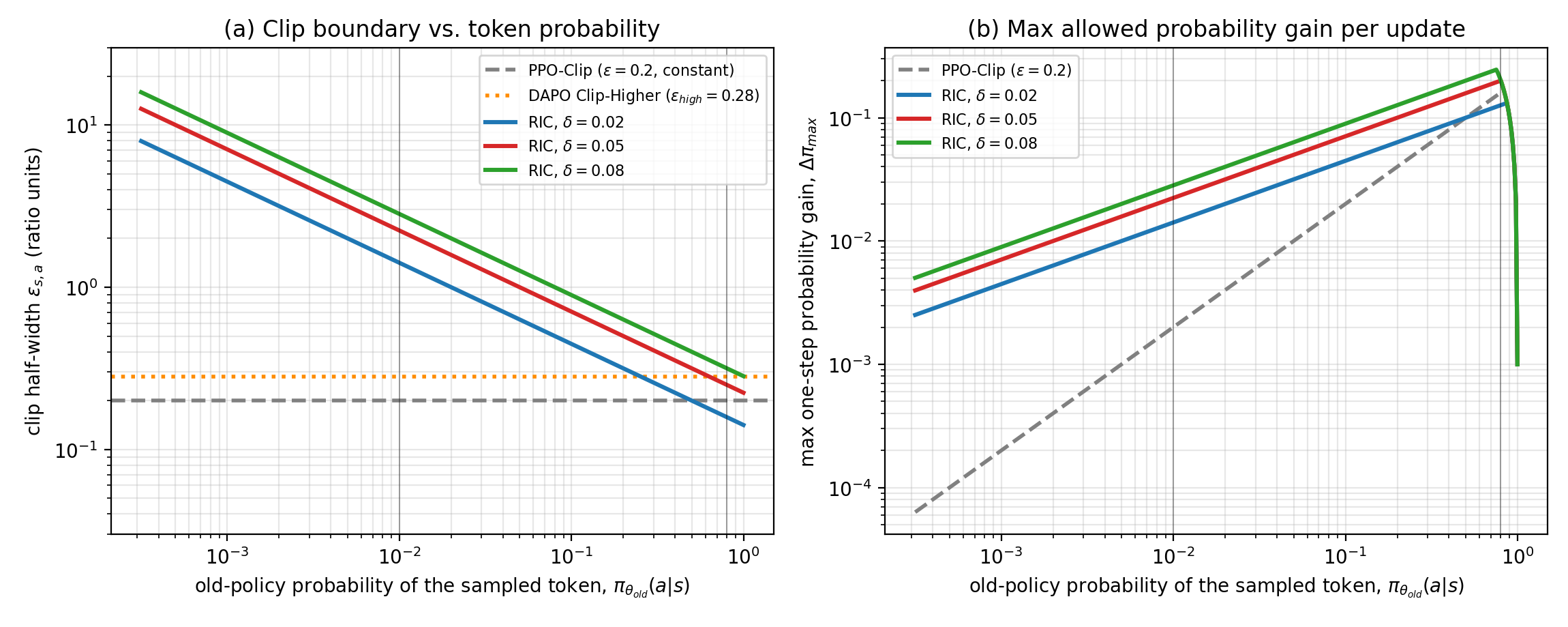
Figure 2 (math visualization, paper Section 3.1 worked example): PPO’s fixed ratio bound $\epsilon=0.2$ allows the high-probability token to gain $0.16$ of absolute probability in one update but the low-probability token only $0.002$ — an 80x difference in absolute update size for the same relative clip width. The chart above generalizes this: panel (a) shows how the clip half-width itself depends on $\pi_{old}$ under RIC (sloping down) versus PPO/DAPO (flat), and panel (b) shows the resulting maximum allowed probability gain — RIC’s curves sit consistently above PPO’s for low-probability tokens and below it for high-probability tokens, exactly the corrective shape the geometric argument predicts.

Even DAPO’s Clip-Higher fix, which raises $\epsilon_{high}$ from $0.2$ to $0.28$, only moves the low-probability token’s cap from $0.012$ to $0.0128$ — still a negligible $0.0008$ absolute gain — while simultaneously letting the high-probability token’s cap rise all the way to $1.0$ ($0.8\times1.28$ clamped at the probability simplex boundary), which intensifies the reduction in behavioral diversity rather than fixing it. This is the paper’s evidence that Clip-Higher (and similar one-sided patches) address the symptom in the wrong direction: they make the already over-permissive side of the clip even more permissive, while barely touching the already over-restrictive side.

Deriving the Geometric Mismatch, Step by Step

Here is the full derivation chain from Equation 4 to the paper’s key inequality (Equation 8), broken into individual algebraic moves so nothing is skipped.

Step 1 — start from the second-order KL expansion (Equation 4 above). Map this from parameter space $\theta$ to the induced space of probability distributions using the chain rule: $\nabla_\theta \pi_\theta(a|s)$ appears when you differentiate $\log \pi_\theta(a|s)$ with respect to $\theta$, giving the Fisher Information Matrix its standard form,

$$F(\theta) = \mathbb{E}_a\left[\nabla_\theta\log\pi_\theta(a|s)\,\nabla_\theta\log\pi_\theta(a|s)^\top\right] = \sum_a \pi_\theta(a|s)\,\frac{\nabla_\theta\pi_\theta(a|s)}{\pi_\theta(a|s)}\frac{\nabla_\theta\pi_\theta(a|s)^\top}{\pi_\theta(a|s)}. \tag{6}$$

Step 2 — substitute into the quadratic form and simplify. Plugging Equation 6 into $\Delta\theta^\top F(\theta)\Delta\theta$ and using $\nabla_\theta\pi_\theta(a|s)^\top\Delta\theta \approx \pi_\theta(a|s) - \pi_{old}(a|s)$ (a first-order Taylor expansion of $\pi_\theta(a|s)$ itself around $\theta_{old}$, Equation 6 in the paper’s numbering) gives

$$2\,D_{KL}(\pi_{old}\|\pi) \approx \sum_a \frac{1}{\pi_{old}(a|s)}\big(\pi(a|s)-\pi_{old}(a|s)\big)^2. \tag{7}$$

Why this substitution is valid: the first-order Taylor expansion $\pi_\theta(a|s)\approx\pi_{old}(a|s)+\nabla_\theta\pi_\theta(a|s)^\top|_{\theta_{old}}\Delta\theta$ is exactly the same linearization used throughout classical policy-gradient theory (it is the same approximation that justifies the policy-gradient theorem itself) — nothing exotic is introduced here, it is standard first-order calculus applied consistently.

Step 3 — factor out $\pi_{old}(a|s)$ to expose the ratio. Divide and multiply the squared term by $\pi_{old}(a|s)^2$: $\frac{(\pi(a|s)-\pi_{old}(a|s))^2}{\pi_{old}(a|s)} = \pi_{old}(a|s)\left(\frac{\pi(a|s)}{\pi_{old}(a|s)}-1\right)^2 = \pi_{old}(a|s)(r_{s,a}-1)^2$. Substituting back gives exactly Equation 5 above (dropping the factor of 2, which the paper absorbs into a redefined constant): $D_{KL}\approx\frac{1}{2}\sum_a \pi_{old}(a|s)(r_{s,a}-1)^2$.

Step 4 — read off the per-token geometric distance. Restricting attention to the single token $a$ that was actually sampled (rather than summing over the whole vocabulary — this restriction is exactly the “Binary”-style simplification that makes the per-token clip tractable), the geometric distance moved by this update is

$$d_{geom}(\pi_{old},\pi) \propto \pi_{old}(a|s)\cdot(r_{s,a}(\theta)-1)^2. \tag{8}$$

Why this single equation is the crux of the entire paper. Compare Equation 8 to what PPO-Clip implicitly measures: $d_{clip}=(r(\theta)-1)^2$ — the same formula, minus the $\pi_{old}(a|s)$ factor. PPO-Clip is not “an approximation with some error” to Equation 8; it is Equation 8 with the entire $\pi_{old}$-dependence silently dropped, which is exactly why the paper calls this a geometric mismatch rather than merely “some noise” or “some slack in an otherwise-correct bound.” A rare token ($\pi_{old}$ tiny) has its true geometric distance shrunk by that tiny factor relative to what PPO-Clip assumes; a dominant token ($\pi_{old}$ near 1) has its true geometric distance essentially un-shrunk, i.e., PPO-Clip under-estimates how much a dominant-token update actually moves the policy, while over-estimating how much a rare-token update moves it.

Quantifying the Mismatch on the Worked Example

Plugging the two example tokens from before into Equation 8, with $r=1.2$ (the ratio at PPO’s clip boundary) for both:

• High-probability token, $\pi_{old}=0.8$: $d_{geom}=0.5\times0.8\times0.2^2=0.016$.
• Low-probability token, $\pi_{old}=0.01$: $d_{geom}=0.5\times0.01\times0.2^2=0.0002$.

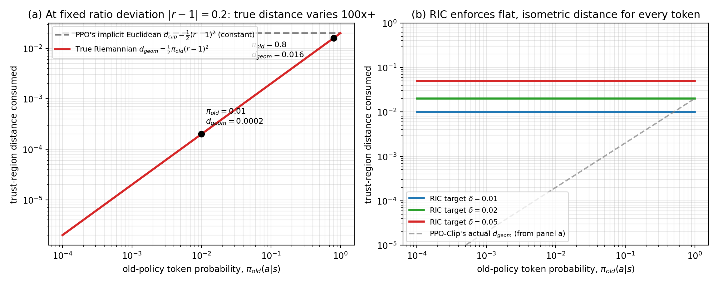
Figure 3 (comparison figure, reproducing the paper’s Section 3.2 illustrative numbers): panel (a) plots the true geometric distance $d_{geom}=\frac{1}{2}\pi_{old}(r-1)^2$ against $\pi_{old}$ at the fixed ratio deviation $|r-1|=0.2$ that PPO-Clip treats as “the same amount of policy change” for every token — the true distance moved differs by 80x between the two marked points ($0.016$ for $\pi_{old}=0.8$ vs. only $0.0002$ for $\pi_{old}=0.01$), while PPO’s implicit assumption (dashed gray) is flat by construction. Panel (b) shows RIC’s fix directly: instead of a flat ratio bound, RIC enforces a flat geometric-distance target (colored horizontal lines) — every token, regardless of its starting probability, consumes the same $\delta$.

The paper states this formally as its central negative result:

Proposition 3.1. PPO-Clip incorrectly employs a Euclidean metric to measure the discrepancy between policies, failing to align with the geometry of the policy Riemannian manifold. This leads to overly conservative updates in low-probability regions while aggressive updates in high-probability regions, ultimately causing exploration collapse.

This is worth restating in plain language because it is easy to read past: PPO-Clip does not fail because $\epsilon=0.2$ is “the wrong number” — no single fixed number could ever be right, because the correct trust-region radius, measured honestly, is not a constant at all; it is a quantity that scales with $\pi_{old}(a|s)$. Any single fixed $\epsilon$, however carefully tuned, will always under-constrain high-probability tokens and over-constrain low-probability ones relative to a true, uniform KL budget. Widening or narrowing $\epsilon$ (as DAPO does) just picks a different point along the same mis-calibrated curve — it cannot fix the shape of the miscalibration itself, only shift it.

flowchart LR
    A["Two tokens, same ratio deviation r=1.2 under PPO-Clip's rule"] --> B1["High-prob token pi_old=0.8"]
    A --> B2["Low-prob token pi_old=0.01"]
    B1 --> C1["True geometric distance: 0.016 (large)"]
    B2 --> C2["True geometric distance: 0.0002 (tiny, 80x smaller)"]
    C1 -.->|"PPO-Clip treats both the same -> under-constrains this one"| D["Exploration collapse:\nhigh-prob tokens swing too freely,\nlow-prob tokens barely move"]
    C2 -.->|"PPO-Clip treats both the same -> over-constrains this one"| D

Figure 4 (data-flow / diagnostic diagram): tracing how one shared clip boundary produces opposite mis-calibrations depending purely on the token’s starting probability — this single mechanism is presented as the paper’s explanation for observed exploration collapse across many independent empirical reports.

Riemannian Isometric Clip (RIC): The Fix, Derived Step by Step

Setting Up the Isometric Constraint

If the true geometric distance of a per-token update is Equation 8, the natural fix is to require every update to consume the same geometric distance, rather than the same ratio deviation:

$$d_{geom}(\pi_{old}(a|s), \pi(a|s)) \triangleq \frac{1}{2}\pi_{old}(a|s)\,(r_{s,a}(\theta)-1)^2 \le \delta. \tag{9}$$

This is Equation 9 in the paper (numbered Eq. 9 in this review, matching the paper’s own Eq. 9). Read it as: “no matter which token this is, do not let the update move it further than $\delta$ in true (Riemannian) trust-region units.”

Solving for the Ratio Bound

Solving Equation 9 for $r_{s,a}(\theta)$ is a two-line algebraic rearrangement, but it is worth doing explicitly since the shape of the final formula is the whole practical contribution:

Step 1. Start from $\frac{1}{2}\pi_{old}(a|s)(r_{s,a}(\theta)-1)^2\le\delta$.

Step 2. Divide both sides by $\frac{1}{2}\pi_{old}(a|s)$ (a positive quantity, so the inequality direction is preserved): $(r_{s,a}(\theta)-1)^2 \le \frac{2\delta}{\pi_{old}(a|s)}$.

Step 3. Take the square root of both sides (valid since both sides are non-negative): $|r_{s,a}(\theta)-1|\le\sqrt{\frac{2\delta}{\pi_{old}(a|s)}}$.

Step 4. Absorb the constant factor of 2 into a redefined $\delta$ (the paper does this explicitly, so the "$\delta$" appearing in the final formula and in all the paper’s experiments already has this factor folded in), giving the final, implementable form:

$$|r_{s,a}(\theta)-1| \le \epsilon_{s,a}(\pi_{old}) = \sqrt{\frac{\delta}{\pi_{old}(a|s)}}. \tag{10}$$

This single closed-form expression, Equation 10, is Riemannian Isometric Clip (RIC). Notice its shape: as $\pi_{old}(a|s)\to 0$ (a very rare token), $\epsilon_{s,a}\to\infty$ — the clip essentially disappears, letting the update through almost unconstrained (because the true geometric cost of moving a near-zero-probability token is itself near zero, however large the ratio looks). As $\pi_{old}(a|s)\to 1$ (an almost-certain token), $\epsilon_{s,a}\to\sqrt{\delta}$ — a small, tight bound (because any ratio movement on a near-certain token corresponds to a large absolute probability swing, which is exactly what a real trust region should restrict).

Why a Square Root, Specifically? Building the Intuition One More Way

It is worth pausing on why the fix takes the specific shape $\epsilon_{s,a}=\sqrt{\delta/\pi_{old}(a|s)}$ — a square-root-of-a-reciprocal — rather than some other monotonically decreasing function of $\pi_{old}$, since the shape is not arbitrary and understanding it makes the formula memorable rather than just derivable.

Reason 1: the quadratic form in Equation 9 forces a square root when solving for $r$. This is the purely algebraic reason (already shown step-by-step above), but it is worth restating why the quadratic (rather than linear) relationship between $d_{geom}$ and $(r-1)$ arises in the first place: it comes directly from the second-order Taylor expansion of KL divergence (Equation 4) — KL divergence has zero gradient at $\pi=\pi_{old}$ (a distribution is at zero divergence from itself, and this is a local minimum), so the leading-order term in its expansion around that point is necessarily quadratic, not linear. Any quantity built from a second-order Taylor expansion of a function at its own minimum will produce a quadratic relationship, and inverting a quadratic relationship for a bound produces a square root — this is the same reason, for instance, that confidence intervals for a variance-normalized quantity scale as $\sqrt{n}$ rather than $n$.

Reason 2: dimensional consistency with “distance”. Think of $\sqrt{\delta/\pi_{old}}$ as playing a role analogous to a standard deviation. If you think of $\pi_{old}(a|s)(r-1)^2$ as being structurally like a squared z-score — (observed deviation)$^2$ / (a scale factor) — then solving for the deviation itself naturally produces a square root, exactly as converting a target variance into a target standard deviation does. This is not a coincidence: the underlying quantity, $\frac{1}{\pi_{old}(a|s)}$, is playing the role of an inverse variance (recall Equation 12’s variance analysis: the variance of an importance-sampling estimator scales as $1/\pi_{old}$ for rare samples) — the same $1/\pi_{old}$ factor that makes rare-sample variance explode in Equation 12 is, up to the square root, exactly the factor that RIC uses to widen the rare-sample clip bound in Equation 10. These are not two unrelated appearances of $1/\pi_{old}$; they are the same statistical fact (rare events carry more “surprise” per observation) showing up in two related places — once as a variance penalty (bad, if unaddressed) and once as a corrected clip bound (the fix).

Reason 3: the two limiting behaviors are exactly what a real trust region should do. As sanity checks at the two extremes: a token with $\pi_{old}\to1$ (the policy is already certain) should have almost no room to move without a large absolute probability change, so the true trust region should be tight — and indeed $\epsilon_{s,a}\to\sqrt{\delta}$, a small constant. A token with $\pi_{old}\to0$ (an essentially never-sampled action) can have its probability multiply by a huge ratio while still moving almost no absolute probability mass, so the true trust region should be loose — and indeed $\epsilon_{s,a}\to\infty$. Both limits match intuition; a linear (rather than square-root) relationship, for comparison, would either overcorrect or undercorrect at one of the two extremes.

Revisiting the Worked Example Under RIC

With $\delta=0.02$ (the paper’s illustrative value for this example):

• High-probability token, $\pi_{old}=0.8$: $\epsilon_{s,a}=\sqrt{0.02/0.8}=\sqrt{0.025}\approx0.158$, giving a maximum updated probability of $0.8\times1.158\approx0.926$ — tighter than PPO-Clip’s $0.96$.
• Low-probability token, $\pi_{old}=0.01$: $\epsilon_{s,a}=\sqrt{0.02/0.01}=\sqrt{2}\approx1.414$, giving a maximum updated probability of $0.01\times2.414\approx0.024$ — more than double PPO-Clip’s $0.012$.

Crucially, both updates now consume exactly $d_{geom}=\delta=0.01$ (after accounting for the factor-of-2 absorbed into $\delta$) of geometric trust-region budget — verified directly by substituting back into Equation 8: $0.5\times0.8\times0.158^2\approx0.01$ and $0.5\times0.01\times1.414^2\approx0.01$. This is the literal meaning of “isometric”: not that the ratio bound is the same (it manifestly is not — $0.158$ vs. $1.414$), but that the geometric distance each update is permitted to move is identical.

flowchart TB
    IN["Per-token update: pi_old(a|s), proposed ratio r"] --> CALC["Compute dynamic clip width:\nepsilon_s,a = sqrt(delta / pi_old(a|s))  Eq.10"]
    CALC --> CHECK{"Is |r - 1| <= epsilon_s,a ?"}
    CHECK -- "yes" --> PASS["Pass gradient through unmodified\n(update consumes <= delta geometric distance)"]
    CHECK -- "no" --> CLIP["Clip r to [1-epsilon_s,a, 1+epsilon_s,a]\n(update capped at exactly delta geometric distance)"]
    PASS --> OUT["Contribute r * A_hat to the RIPO objective, Eq.11"]
    CLIP --> OUT

Figure 5 (data-flow / pipeline diagram): the complete per-token decision procedure for Riemannian Isometric Clip. Unlike PPO’s single global $\epsilon$, the clip width here is recomputed per token from that token’s own $\pi_{old}(a|s)$ — the only new computation is a square root of two already-available scalars.

The Full RIPO Objective

Plugging RIC (Equation 10) into the GRPO objective (in place of GRPO’s fixed $\epsilon$) gives the complete RIPO training objective:

$$J_{RIPO}(\theta) = \mathbb{E}_{q\sim D,\{o_i\}_{i=1}^G\sim\pi_{\theta_{old}}(\cdot|q)}\left[\frac{1}{\sum_{i=1}^G|o_i|}\sum_{i=1}^G\sum_{t=1}^{|o_i|}\min\Big(r_{i,t}(\theta)\hat{A}_{i,t},\ \operatorname{clip}\big(r_{i,t}(\theta),\,1-\epsilon_{i,t}(\pi_{\theta_{old}}),\,1+\epsilon_{i,t}(\pi_{\theta_{old}})\big)\hat{A}_{i,t}\Big)\right]. \tag{11}$$

Note everything that is unchanged relative to GRPO’s original objective (Equation 2 of the “Prerequisites” section): the group-relative advantage $\hat{A}_{i,t}$ (Equation 3), the token-level loss aggregation, the min-of-clipped-and-unclipped structure. The only change is that the single scalar $\epsilon$ becomes the per-token function $\epsilon_{i,t}(\pi_{\theta_{old}})=\sqrt{\delta/\pi_{\theta_{old}}(o_{i,t}|q,o_{i,<t})}$. This is exactly why the paper can present RIPO as a near-drop-in replacement: the surrounding training loop — rollout collection, reward scoring, advantage computation, gradient aggregation — is completely untouched.

Pseudocode (per-token RIC masking inside a GRPO/PPO training step):

for each response o_i sampled from behavior policy pi_theta_old:
    for t in 1..|o_i|:
        pi_old_t   = pi_theta_old(o_i[t] | q, o_i[:t])       # already computed for the ratio anyway
        pi_new_t   = pi_theta(o_i[t] | q, o_i[:t])           # already computed for the ratio anyway
        r_t        = pi_new_t / pi_old_t
        eps_t      = sqrt(delta / pi_old_t)                  # THE ONLY NEW COMPUTATION: one sqrt, one divide
        r_clipped  = clip(r_t, 1 - eps_t, 1 + eps_t)
        term_t     = min(r_t * A_hat_i, r_clipped * A_hat_i)  # same min-structure as vanilla PPO/GRPO
    loss += -mean_t(term_t) over all tokens in this response
loss = mean over all responses in the group (token-mean aggregation, as in DAPO)

The implementation footprint is genuinely tiny: eps_t = sqrt(delta / pi_old_t) replaces a single constant eps = 0.2 in an existing PPO/GRPO codebase — everything else (data collection, reward scoring, advantage estimation, the min/clip structure itself) is byte-for-byte identical to the baseline. This is worth emphasizing because it directly explains why the paper’s experimental section can run so many configurations (four model families, seven benchmarks, PPO transfer, coding/search generalization) — the change being tested is genuinely orthogonal to everything else in the pipeline, so each experiment is a clean, controlled swap of one line.

Why the “Dual Clipping” Detail Matters

One implementation detail the paper carries over from prior work (Ye et al., 2020; used by DAPO, DCPO, and now RIPO) is dual clipping: in addition to the upper/lower bounds from Equation 10, the ratio is further hard-clamped to an absolute range, here $[0.5, 10]$. Why is this necessary even with RIC’s dynamic bound? Consider a token with $\pi_{old}(a|s)=10^{-6}$ (an extremely rare token, plausible in a 150k-token vocabulary over a long sequence): Equation 10 gives $\epsilon_{s,a}=\sqrt{\delta/10^{-6}}$, which for $\delta=0.05$ is $\epsilon_{s,a}\approx 224$ — an enormous, practically unbounded clip width. Without an absolute ceiling, a single extremely rare token could in principle receive an astronomically large gradient weight if its ratio happened to spike, which would reintroduce a different kind of instability (numerical, not geometric) that Equation 10 alone does not guard against. The dual clip at $[0.5,10]$ is a pragmatic safety rail on top of the geometrically-motivated bound — it does not change RIC’s core logic for any token whose old probability is not vanishingly small, but it prevents pathological gradient spikes at the extreme tail.

A Runnable Reference Implementation

Because the pseudocode above deliberately stays close to plain English, it is worth also showing the change as it would actually appear inside a PyTorch training step, so the “this is a one-line patch” claim can be checked directly against code rather than taken on faith. The snippet below assumes log_pi_old and log_pi_new are already computed per-token log-probabilities (as any PPO/GRPO implementation already computes to form the ratio), and that advantages and delta (the trust-region budget, a single scalar hyperparameter) are given:

import torch

def ppo_clip_loss(log_pi_new, log_pi_old, advantages, eps=0.2, dual_clip=10.0):
    """Baseline PPO/GRPO clip: one fixed eps for every token."""
    ratio = torch.exp(log_pi_new - log_pi_old)
    unclipped = ratio * advantages
    clipped = torch.clamp(ratio, 1 - eps, 1 + eps) * advantages
    # dual clip: hard absolute ceiling on the ratio itself, applied on top
    surrogate = torch.min(unclipped, clipped)
    surrogate = torch.where(ratio > dual_clip, torch.min(surrogate, advantages), surrogate)
    return -surrogate.mean()


def ripo_clip_loss(log_pi_new, log_pi_old, advantages, delta=0.05, dual_clip=(0.5, 10.0)):
    """RIPO / RIC clip: eps_t is now a per-token function of pi_old."""
    pi_old = torch.exp(log_pi_old)                          # THE ONLY NEW TENSOR
    ratio = torch.exp(log_pi_new - log_pi_old)
    eps_t = torch.sqrt(delta / pi_old.clamp_min(1e-12))      # Equation 10, per token
    lower, upper = 1 - eps_t, 1 + eps_t
    unclipped = ratio * advantages
    clipped = torch.clamp(ratio, lower, upper) * advantages
    surrogate = torch.min(unclipped, clipped)
    # dual clip is now an absolute floor/ceiling on the raw ratio, unchanged from PPO-Clip
    lo, hi = dual_clip
    surrogate = torch.where((ratio < lo) | (ratio > hi), torch.min(surrogate, advantages), surrogate)
    return -surrogate.mean()

Reading the diff between the two functions line-by-line: ppo_clip_loss and ripo_clip_loss are identical except for exactly three lines — the new pi_old tensor, the eps_t = torch.sqrt(...) line that replaces the constant eps, and using lower, upper (now tensors, one value per token in the batch) instead of 1 - eps, 1 + eps (scalars, broadcast identically to every token) inside torch.clamp. Every other line — the ratio computation, the unclipped/clipped surrogate construction, the min-of-two structure, the dual-clip safety rail, the final mean-and-negate — is byte-for-byte the same function body. This is the clearest possible demonstration of the paper’s claim that RIC is a corrected formula, not a new algorithm: a code reviewer diffing these two functions would see a three-line change, not a rewrite.

A Fully Worked Mini-Batch Trace

To make the token-level mechanics fully concrete (rather than only stating the general shapes above), here is one complete forward pass through both ppo_clip_loss and ripo_clip_loss on a tiny hand-picked mini-batch of four tokens, chosen to straddle the paper’s own $\delta=0.02$ crossover point (the old-policy probability at which RIC’s bound exactly equals PPO’s fixed $\epsilon=0.2$, which algebraically is $\pi_{old}=\delta/\epsilon^2=0.02/0.04=0.5$ — below this probability RIC is wider than PPO, above it RIC is narrower). Assume all four tokens happen to have ratio $r=\pi_{new}/\pi_{old}=1.1$ (a 10% probability increase relative to the old policy — the same ratio for every token, so any difference in outcome is due entirely to the clip boundary, not to the ratio itself) and advantage $\hat{A}=+1$ for all four (a positive-advantage action, so the surrogate objective wants to increase this token’s probability), with PPO’s fixed $\epsilon=0.2$ and RIPO’s $\delta=0.02$ (the paper’s own illustrative value):

Token	$\pi_{old}$	$r$	PPO-Clip $[\text{lo},\text{hi}]$	PPO clips?	RIPO $\epsilon_{s,a}=\sqrt{\delta/\pi_{old}}$	RIPO $[\text{lo},\text{hi}]$	RIPO clips?
A (very rare)	0.001	1.1	$[0.8, 1.2]$	No (1.1 inside)	$\sqrt{20}\approx4.472$	$[-3.472, 5.472]$	No
B (rare)	0.02	1.1	$[0.8, 1.2]$	No (1.1 inside)	$\sqrt{1}=1.000$	$[0.000, 2.000]$	No
C (past crossover)	0.6	1.1	$[0.8, 1.2]$	No (1.1 inside)	$\sqrt{0.0333}\approx0.183$	$[0.817, 1.183]$	No
D (dominant)	0.9	1.1	$[0.8, 1.2]$	No (1.1 inside)	$\sqrt{0.0222}\approx0.149$	$[0.851, 1.149]$	No

At first glance this trace looks unremarkable — with $r=1.1$ comfortably inside both PPO’s $[0.8,1.2]$ band and every token’s RIC band, none of the four gets clipped under either scheme, so the gradient step is identical (unclipped $r\hat{A}=1.1$) for all four tokens under both methods. This is the correct and important observation for this particular ratio: RIC does not change anything for moderate ratio deviations that already sit safely inside both bounds — its effect is concentrated at the boundary. Now repeat the exact same trace but push every token to a larger ratio, $r=1.3$ (a 30% increase, enough to exceed PPO’s boundary for all four and RIC’s boundary for tokens C and D, while remaining inside RIC’s much wider boundary for tokens A and B), to see exactly where the two methods diverge:

Token	$\pi_{old}$	$r$	PPO clips at $1.2$?	Surrogate kept (PPO)	RIPO clips at?	Surrogate kept (RIPO)
A (very rare)	0.001	1.3	Yes	$\min(1.3,1.2)=1.2$	No — RIPO’s upper bound is $5.472$, far above $1.3$	$\min(1.3,5.472)=1.3$ (unclipped — full gradient)
B (rare)	0.02	1.3	Yes	$1.2$	No — RIPO’s upper bound is $2.000$	$1.3$ (unclipped)
C (past crossover)	0.6	1.3	Yes	$1.2$	Yes — RIPO’s upper bound is $1.183$	$\min(1.3,1.183)=1.183$
D (dominant)	0.9	1.3	Yes	$1.2$	Yes — RIPO’s upper bound is $1.149$	$\min(1.3,1.149)=1.149$

This second trace is exactly the mechanism the paper’s worked example (Section 3.1) describes in the abstract, now shown as an explicit forward pass with a full arithmetic audit trail: PPO-Clip treats all four tokens identically — every one of them gets clipped at the same $1+\epsilon=1.2$ boundary and contributes the exact same $1.2\times\hat{A}=1.2$ surrogate value, regardless of whether the token was a one-in-a-thousand rare event (A) or already the dominant next-token choice 90% of the time (D). RIPO-Clip treats all four tokens differently, in exactly the direction the paper argues is correct, and the split falls exactly at the $\pi_{old}=0.5$ crossover point derived above: tokens A and B (both $\pi_{old}<0.5$) — the rare, exploration-relevant tokens — sail through completely unclipped and keep their full surrogate value ($1.3$, about $8.3\%$ larger than what PPO would have kept), while tokens C and D (both $\pi_{old}>0.5$) — the already-common tokens — still get clipped, at boundaries ($1.183$ and $1.149$) that are tighter than PPO’s uniform $1.2$, not looser. The net effect on this batch: RIPO preserves 100% of the gradient magnitude on the two rare tokens where PPO was silently truncating it, while simultaneously reining in the two common tokens more aggressively than PPO’s one-size-fits-all boundary — the same single formula (Equation 10) produces both corrections at once, because both are the same geometric fact viewed from opposite sides of the crossover point.

Theory: Why Isometric Updates Also Fix a Variance Problem

This section explains a second, less obvious benefit of RIC that the paper derives as a consequence of the same geometric argument: a favorable bias–variance trade-off for the underlying importance-sampling estimator.

The Variance Problem in Off-Policy Estimation

For an off-policy objective estimated via importance sampling, $\mathbb{E}_{x\sim\pi}[A(x)]=\mathbb{E}_{x\sim\pi_{old}}[r(x)A(x)]$ — this identity is unbiased but can have enormous variance. The variance is dominated by the second-moment term (the squared-mean term is comparatively negligible, a standard result in importance-sampling theory):

$$\mathbb{V}_{x\sim\pi_{old}}[r(x)A(x)] \approx \mathbb{E}_{x\sim\pi_{old}}\big[r(x)^2A(x)^2\big] = \sum_x \pi_{old}(x)\,r(x)^2 A(x)^2. \tag{12}$$

Why the variance explodes: define the per-sample variance contribution $v(x)=\pi_{old}(x)r(x)^2=\pi_{old}(x)\cdot\big(\pi(x)/\pi_{old}(x)\big)^2=\pi(x)^2/\pi_{old}(x)$. As $\pi_{old}(x)\to0$ for a rare sample $x$, this quantity blows up — the classic long-tail pathology of importance sampling, where rare events with large ratios dominate (and destabilize) the variance.

How PPO-Clip Handles This — Trading Bias for Variance

PPO-Clip’s truncation $r(x)\le1+\epsilon$ mitigates the variance explosion for free: for a sample near the clipped boundary, $v(x')=\pi_{old}(x')(1+\epsilon)^2\to0$ as $\pi_{old}(x')\to0$, since the ratio is capped rather than allowed to grow unboundedly. But this comes at a cost the paper is explicit about: clipping discards the contribution of these samples to the objective entirely, introducing bias in exchange for the variance reduction. This is a real trade-off, not a free lunch — PPO-Clip is choosing low variance at the price of higher bias on exactly the rare, informative samples that matter most for exploration.

How RIC Achieves Lower Variance and Lower Bias Simultaneously

RIC’s distribution-dependent threshold $r(x)\le1+\sqrt{\delta/\pi_{old}(x)}$ changes the calculation. The variance contribution of a sample near this clipped boundary is:

$$v(x') = \pi_{old}(x')\left(1+\sqrt{\frac{\delta}{\pi_{old}(x')}}\right)^2 \approx \pi_{old}(x')\cdot\frac{\delta}{\pi_{old}(x')} = O(\delta), \tag{13}$$

Working through this approximation explicitly: expand the square, $\left(1+\sqrt{\delta/\pi_{old}(x')}\right)^2 = 1 + 2\sqrt{\delta/\pi_{old}(x')} + \delta/\pi_{old}(x')$. For small $\pi_{old}(x')$, the last term dominates (it blows up as $\pi_{old}(x')\to0$, while the other two terms stay bounded), so $v(x')\approx\pi_{old}(x')\cdot\delta/\pi_{old}(x') = \delta$ — the $\pi_{old}(x')$ factor exactly cancels the blow-up in the dominant term, leaving a variance contribution that is constant ($O(\delta)$) regardless of how rare the sample is. This constant-variance property is called statistical homoscedasticity — the variance is the same across the whole range of $\pi_{old}$ values, as opposed to PPO-Clip’s heteroscedastic (probability-dependent) variance.

Why this matters practically: because RIC’s variance is bounded by a constant $O(\delta)$ without needing to discard rare samples the way PPO-Clip’s fixed threshold does — RIC still constrains rare-token updates, but at a threshold that scales with $1/\sqrt{\pi_{old}}$ rather than being fixed, so more rare-but-informative samples survive un-clipped while variance stays controlled. This is the formal justification for why RIC simultaneously reduces both the exploration-collapse bias problem and the variance-explosion problem — they turn out to be two symptoms of the same underlying Euclidean-vs-Riemannian mismatch, and fixing the geometry fixes both at once.

Figure 6 (math visualization of the variance derivation): PPO-Clip’s variance contribution near its clip boundary is $\pi_{old}(x')(1+\epsilon)^2$, which vanishes as $\pi_{old}(x')\to0$ only because the fixed threshold $\epsilon$ eventually clips away the entire rare-sample contribution. RIC’s variance contribution stays flat at $O(\delta)$ across all $\pi_{old}(x')$ by construction — this is the algebraic content of “geometric isometry implies statistical homoscedasticity” (paper Section 4.2).

A Worked Numeric Table for the Homoscedasticity Claim

To make Equation 13’s “constant $O(\delta)$” claim concrete rather than purely symbolic, here is the actual variance-contribution number at the clip boundary for several values of $\pi_{old}(x')$, using $\delta=0.05$ and comparing against PPO-Clip’s $\epsilon=0.2$:

$\pi_{old}(x')$	PPO-Clip’s $\epsilon_{s,a}$ (fixed)	PPO-Clip’s $v(x')=\pi_{old}(1+\epsilon)^2$	RIC’s $\epsilon_{s,a}=\sqrt{\delta/\pi_{old}}$	RIC’s $v(x')\approx\delta$
$0.5$	$0.2$	$0.5\times1.44=0.72$	$\sqrt{0.1}\approx0.316$	$\approx0.05$
$0.1$	$0.2$	$0.1\times1.44=0.144$	$\sqrt{0.5}\approx0.707$	$\approx0.05$
$0.01$	$0.2$	$0.01\times1.44=0.0144$	$\sqrt{5}\approx2.236$	$\approx0.05$
$0.001$	$0.2$	$0.001\times1.44=0.00144$	$\sqrt{50}\approx7.07$	$\approx0.05$
$0.0001$	$0.2$	$0.0001\times1.44=0.000144$	$\sqrt{500}\approx22.4$	$\approx0.05$

Read the last two columns together: RIC’s clip width genuinely explodes for very rare tokens (as it must, per the earlier discussion of why the dual absolute clip $[0.5,10]$ is still needed as a safety rail) — but its variance contribution stays essentially pinned at $\delta=0.05$ across four orders of magnitude of $\pi_{old}$. PPO-Clip’s variance contribution, by contrast, shrinks by four orders of magnitude over the same range (from $0.72$ down to $0.000144$) — which sounds like a good thing (lower variance!) until you recall from the main derivation that this apparent variance reduction is bought entirely by discarding the rare sample’s contribution to the objective (the bias side of the trade-off), not by any genuine improvement in estimation quality.

Experiments: Dissecting Where RIPO’s Gains Come From

The paper runs a genuinely broad sweep of experiments, moving from the headline math-reasoning comparison to targeted diagnostics that isolate why RIPO wins, then checks generalization beyond math. I walk through each in turn.

Experimental Setup

• Models: Qwen3-1.7B-Base, Qwen3-4B-Base, Qwen3-8B-Base, Llama3.2-3B-Instruct — spanning two model families and roughly a 5x parameter range.
• Baselines: GRPO (vanilla PPO-Clip), DAPO (Clip-Higher), GSPO (sequence-level clipping), GMPO (geometric-mean ratio clipping), DCPO (dynamic-adaptive clipping) — five distinct prior clipping mechanisms, all sharing GRPO’s group-relative advantage estimator.
• Training data: DAPO-Math-17k (17,917 questions), 8 rollouts per question, max response length 16,384 tokens, 1,024 rollouts per RL iteration (train batch size 128, 8 gradient updates per batch with mini-batch size 16), 300 steps to convergence, AdamW at constant LR $10^{-6}$, on VeRL, 8×A100 GPUs. KL penalty removed for all methods (standard practice per DAPO/DCPO), dual clip $[0.5,10]$ applied to GRPO/DAPO/DCPO/RIPO.
• Evaluation: seven decontaminated competition-level math benchmarks — AIME24, AIME25, AMC23, HMMT25, BRUMO25, CMIMC25, SMT25 — evaluated at Avg@8 (8 samples per problem, averaged) for stability.
• RIPO’s one hyperparameter: $\delta=0.05$ by default (symmetric upper/lower budget).

Main Result: Table 1, Reproduced

Method	Qwen3-1.7B-Base	Llama3.2-3B-Instruct	Qwen3-4B-Base	Qwen3-8B-Base
Base (no RL)	6.9	3.5	13.8	11.5
GRPO	11.2	6.4	25.7	28.5
DAPO	12.4 (+10.7%)	7.4 (+15.6%)	27.1 (+5.4%)	30.6 (+7.4%)
GSPO	13.3 (+19.0%)	7.2 (+12.5%)	26.8 (+4.3%)	32.1 (+12.6%)
GMPO	13.9 (+24.1%)	7.4 (+15.6%)	28.4 (+10.5%)	35.3 (+23.9%)
DCPO	14.8 (+32.1%)	6.9 (+7.8%)	27.8 (+8.2%)	34.5 (+21.1%)
RIPO	15.4 (+37.2%)	8.6 (+34.4%)	30.1 (+17.1%)	38.5 (+35.1%)

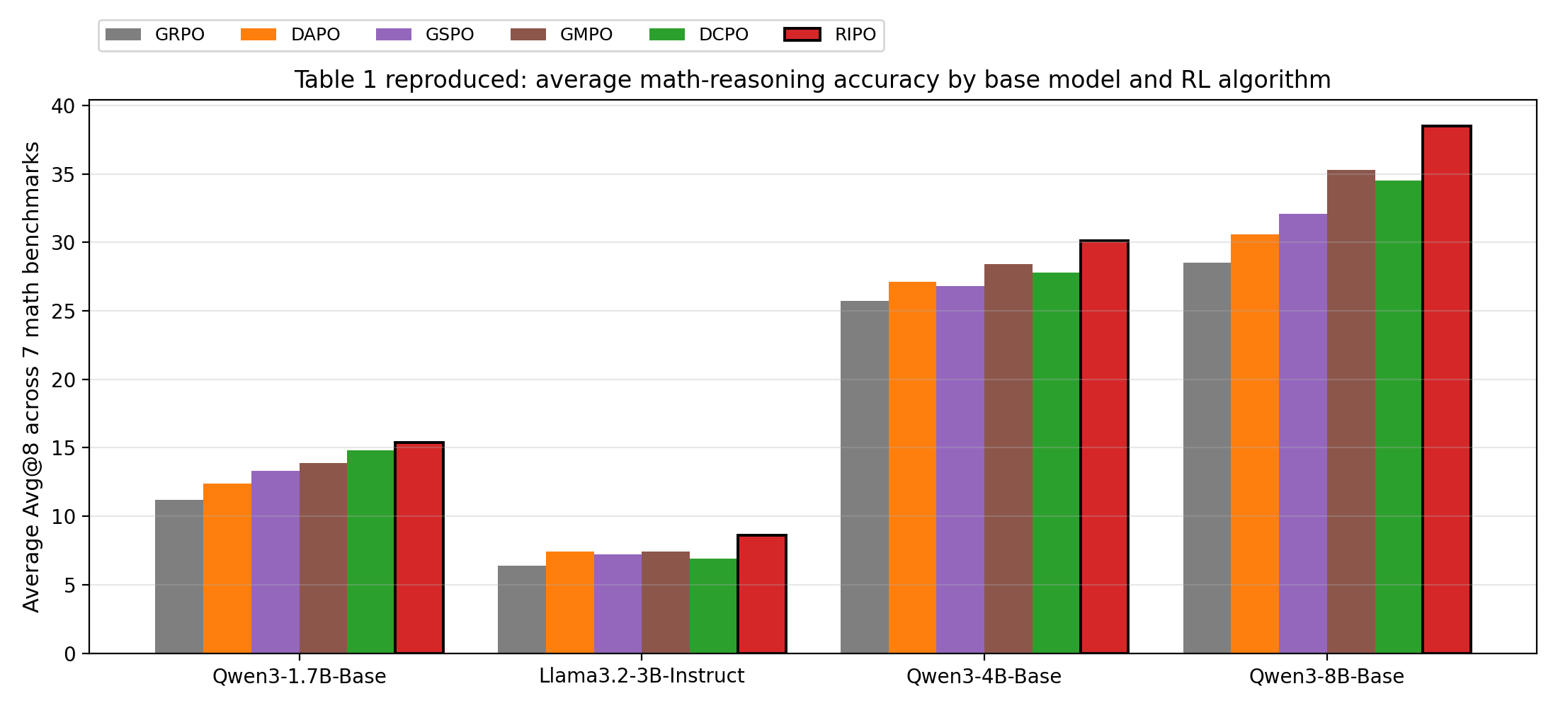
Figure 7 (paper Table 1, reproduced as bar chart above): average Avg@8 across all seven math benchmarks, by base model and RL algorithm. Percentages are relative improvement over GRPO on the same base model. RIPO is the best method on every single base model, and its margin over the next-best baseline widens on the larger models (Qwen3-4B/8B), suggesting the geometric mismatch matters more, not less, as models scale.

The pattern worth dwelling on: RIPO’s advantage grows with model size relative to GRPO (37.2% → 34.4% → 17.1% → 35.1%, non-monotonic across model families but never small), and specifically widens on the hardest benchmarks (AIME24, BRUMO25) relative to easier ones (AMC23). This is exactly what the paper’s diagnosis would predict: harder problems require more genuine exploration of rare-but-correct reasoning paths, which is precisely the regime where the ratio-vs-geometric-distance mismatch (Equation 8) is largest in absolute terms.

RQ: What Do the Training Dynamics Actually Look Like?

Rather than only reporting final numbers, the paper visualizes four training-dynamics signals for Qwen3-8B-Base across all six methods:

Figure 8 (paper Fig. 1, training dynamics — reproduced from the source PDF): (a) evaluation accuracy on AIME24 over training steps; (b) policy entropy; (c) gradient norm; (d) proportion of clipped tokens.

Reading each panel in turn:

(a) Evaluation accuracy. RIPO (red) reaches GRPO’s 200-step accuracy within only 40 steps — the paper calls this “five times the token-efficiency” — and its curve rises smoothly without the abrupt drops visible in some other methods’ curves, meaning RIPO does not experience a mid-training collapse-and-recover pattern.

(b) Policy entropy. This is the most direct visual confirmation of the exploration-collapse diagnosis. GRPO’s entropy (blue) collapses rapidly toward near-zero — the policy becomes almost deterministic, i.e., stops exploring. DAPO’s entropy (orange) does the opposite and grows essentially uncontrolled, which the paper interprets as excessive, destabilizing exploration (Clip-Higher over-corrects). RIPO’s entropy decreases initially (normal, expected exploitation of easy gains early in training) then stabilizes at a moderate, non-zero level — neither collapsing nor exploding, exactly the “sustained but bounded exploration” the geometric argument predicts.

(c) Gradient norm. Every other method shows pronounced oscillations and occasional sharp spikes (visually most extreme for DAPO, consistent with panel (b)‘s entropy explosion). RIPO’s gradient norm is nearly flat throughout training — direct empirical support for the homoscedastic-variance argument in Equation 13: if the variance contribution per clipped sample is genuinely constant, the aggregate gradient norm should indeed be more stable than under a heteroscedastic estimator.

(d) Clipped-token proportion. DCPO and GMPO rarely trigger their clip at all (very low clip ratio); GSPO and DAPO clip orders of magnitude more tokens. RIPO sits in between these extremes — the paper reads this as evidence RIPO’s trust region is “well-calibrated”: neither so loose that it never engages (risking the instability that motivated trust regions in the first place) nor so tight that it constantly fires (risking the original exploration-collapse problem).

Ablation: How Sensitive Is RIPO to Its One New Hyperparameter?

$\delta_{low}$	0.02	0.05	0.05	0.08	0.05	0.08	0.08
$\delta_{high}$	0.02	0.04	0.05	0.08	0.02	0.02	0.04
Avg@8 (AIME24)	40.8	41.7	43.8	42.1	28.8	27.5	27.9

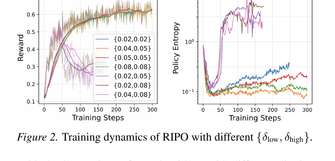
Figure 9 (paper Table 2 + Figure 2, reproduced from the source PDF): RIPO’s reward and entropy training curves under seven different $\{\delta_{low},\delta_{high}\}$ configurations.

The result splits cleanly into two regimes. Symmetric or mildly asymmetric $\delta$ values ($0.02$ to $0.08$, with $\delta_{low}\approx\delta_{high}$) all land within a narrow $40.8$–$43.8$ Avg@8 band — genuinely robust to the exact value chosen, which matters practically because it means $\delta$ does not need expensive per-task tuning. Highly asymmetric configurations ($\delta_{low}=0.02,\delta_{high}=0.08$ or similar) collapse to $27$–$29$ Avg@8 — a large, sudden drop. The paper’s explanation, visible directly in the reward/entropy curves (Figure 9 panel (b)): asymmetric clipping “makes action probabilities much easier to increase than to decrease,” so a token whose probability should be falling instead keeps rising unchecked, producing an entropy explosion and consequent reward collapse. The design lesson: a well-calibrated trust region must constrain both directions of probability movement in a matched way — over-relaxing one side while leaving the other tight reintroduces a new, asymmetric version of exactly the mismatch problem RIPO was built to eliminate.

Comparison with Other Clipping Motivations (Table 3)

Benchmark	GRPO	GPPO	Clip-Cov	RIPO
AIME24	31.7	31.7 (+0.0%)	36.3 (+4.6%)	43.8 (+12.1%)
AIME25	20.8	23.8 (+3.0%)	22.9 (+2.1%)	29.2 (+8.4%)
AMC23	66.6	73.4 (+6.8%)	66.6 (+0.0%)	79.7 (+13.1%)
HMMT25	12.9	14.2 (+1.3%)	11.7 (−1.2%)	16.7 (+3.8%)
BRUMO25	33.3	38.3 (+5.0%)	36.3 (+3.0%)	47.5 (+14.2%)
SMT25	21.9	25.0 (+3.1%)	30.2 (+8.3%)	34.2 (+14.2%)

GPPO (preserves gradients on clipped tokens rather than zeroing them) and Clip-Cov (clips high-covariance tokens to regulate entropy) each represent a genuinely different motivation for modifying the clip than RIC’s geometric argument. Both show modest, inconsistent gains over GRPO (Clip-Cov even loses slightly on HMMT25). RIPO’s margin over both is substantially larger and consistent across every benchmark — evidence that a principled geometric re-derivation outperforms heuristics aimed at related but distinct symptoms (gradient information loss, entropy regulation) of the same underlying miscalibration.

Transfer to the PPO Objective (Table 4)

To check whether RIC’s benefit is specific to GRPO’s group-relative advantage or a property of the clip itself, the paper swaps RIC into vanilla PPO (with a learned value model and GAE, Qwen2.5-Instruct, GSM8K, Avg@1):

Model size	PPO-Clip	DAPO-Clip	DCPO-Clip	RIPO-Clip
0.5B	58.0	58.7 (+0.7)	58.4 (+0.4)	61.1 (+3.1)
1.5B	79.2	80.9 (+1.7)	79.6 (+0.4)	81.6 (+2.4)
7B	91.7	90.8 (−0.9)	91.4 (−0.3)	93.5 (+1.8)
14B	93.2	93.6 (+0.4)	93.9 (+0.7)	94.4 (+1.2)

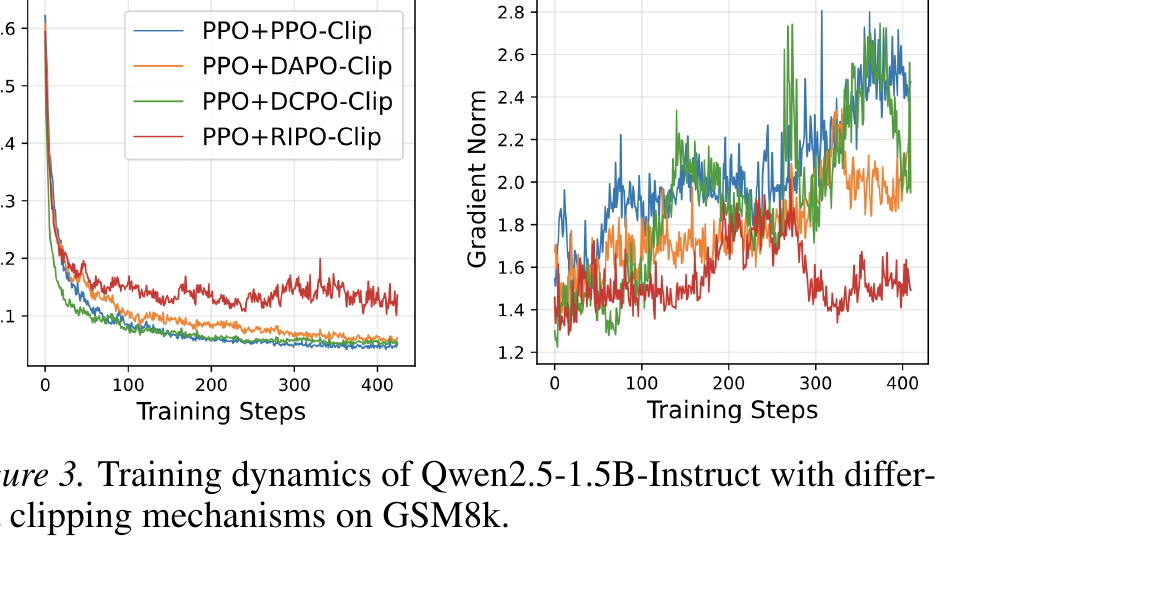
Figure 10 (paper Table 4 + Figure 3, reproduced from the source PDF): training dynamics of Qwen2.5-1.5B-Instruct under different clipping mechanisms on GSM8K, showing PPO-Clip’s severe entropy collapse to near-zero versus RIPO-Clip’s sustained moderate entropy, and PPO/DAPO/DCPO’s growing gradient-norm oscillations versus RIPO-Clip’s comparatively smooth gradient norm.

Notice DAPO-Clip and DCPO-Clip actually underperform vanilla PPO-Clip at 7B (negative deltas) — a reminder that heuristic clip modifications are not universally beneficial and can regress depending on model scale and objective. RIPO-Clip is positive at every scale tested, from 0.5B to 14B, which is the paper’s strongest evidence that the benefit comes from the clip’s geometry being corrected, not from anything specific to GRPO’s advantage estimator or to the particular model family used in the main experiments.

Pass@k: Does RIPO Raise the Capability Ceiling, or Just Pick Winners Faster?

A natural skeptical question about any RL method: does it genuinely expand what the model can do, or does it just make an already-latent capability easier to sample (i.e., would enough random sampling from the base/GRPO model eventually match it)? The paper checks this with a deep Pass@k sweep up to $k=128$ on the two hardest benchmarks:

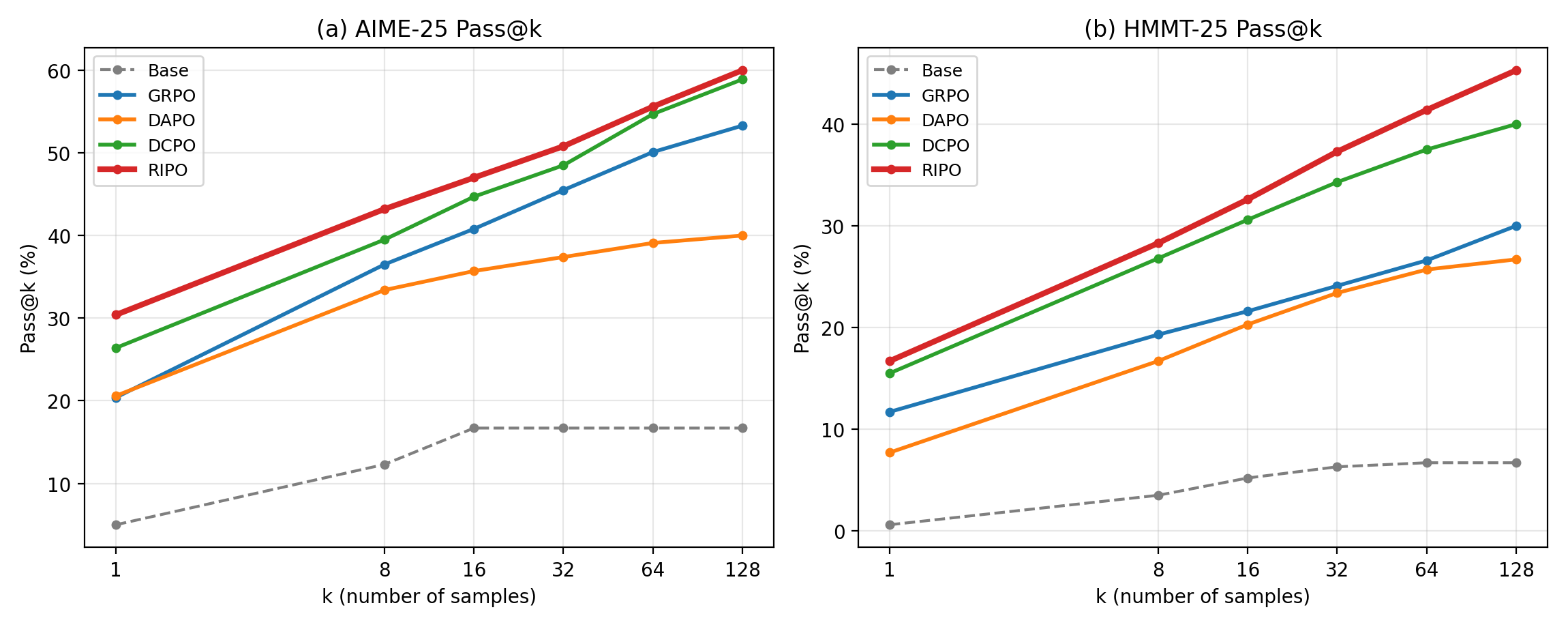
Figure 11 (paper Table 5, reproduced as line charts above): Pass@k curves for AIME-25 and HMMT-25, $k\in\{1,8,16,32,64,128\}$, comparing Base, GRPO, DAPO, DCPO, and RIPO.

The base model’s Pass@k curve plateaus by around $k=16$ on both benchmarks — sampling more from the un-tuned model simply does not find additional correct solutions past that point, indicating a genuine capacity ceiling, not just a sampling-budget problem. GRPO, DAPO, and DCPO all raise this ceiling somewhat but still show diminishing returns by $k=64$–$128$. RIPO’s curve keeps climbing all the way to $k=128$ (reaching 60.0% on AIME-25 and 45.3% on HMMT-25, both the highest of any method at every $k$ value tested) — this is direct evidence that RIPO is not merely re-ranking existing capability more efficiently, it is genuinely expanding the set of correct reasoning paths the policy can reach, which is exactly the claim that “fixing exploration collapse” should predict: a policy that explores more broadly during training should end up able to produce a more diverse — and hence larger, at high sampling budgets — set of valid solutions.

Generalization Beyond Math: Coding and Multi-Hop Search

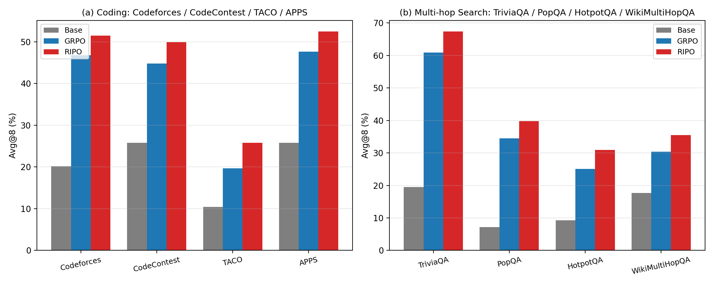
Figure 12 (paper Table 6, reproduced as grouped bar charts above): Avg@8 on four coding benchmarks (Codeforces, CodeContest, TACO, APPS; trained on Eurus-Code) and four multi-hop search benchmarks (TriviaQA, PopQA, HotpotQA, WikiMultiHopQA; trained on Search-R1), comparing Base, GRPO, and RIPO on Qwen3-8B-Base.

RIPO beats GRPO by 13.2% relative on the coding average and 15.1% relative on the search average — comparable in magnitude to the math-reasoning gains, and notably these are qualitatively different task families (competitive programming judged by test-case pass/fail; multi-hop question answering with an external search tool in the loop). The consistency of the gain across math, code, and search is the paper’s evidence that the mechanism it identifies — long-tailed token distributions making the ratio a poor proxy for real distributional change — is a general property of LLM generation, not an artifact specific to mathematical chain-of-thought.

Why Should a Math-Motivated Fix Transfer to Code and Search At All?

It is worth pausing on why this transfer is not obvious a priori, since the paper’s core diagnostic example (Section 3.1) is phrased entirely in terms of mathematical reasoning tokens. The argument that makes the transfer plausible rests on identifying what property of math token distributions the paper’s mechanism actually depends on, and then checking whether code and search share that property:

• The mechanism depends on long-tailed, skewed token probabilities — not on mathematical content per se. Equation 8’s geometric mismatch, $d_{geom}\propto\pi_{old}(a|s)\cdot(r-1)^2$, is a statement about any token whose old-policy probability is small; it never references what the token semantically represents. What made the math-reasoning setting a good testbed is that chain-of-thought math generation happens to have an especially long-tailed vocabulary: rare tokens correspond to specific numerical values, uncommon derivation steps, or infrequently-used symbolic manipulations, all of which are individually rare but collectively make up a large share of what separates a correct proof path from an incorrect one.
• Code generation has an analogous — arguably sharper — long tail. A correct program frequently depends on selecting one specific, rarely-used API call, an uncommon standard-library function, or an unusual-but-necessary edge-case branch (e.g., a specific exception type, a rarely-invoked helper). These tokens are exactly the kind PPO-Clip’s uniform $\epsilon=0.2$ under-explores: they are individually improbable under the old policy but often decisive for whether the generated program passes the test suite (Codeforces, CodeContest, TACO, APPS are all pass/fail judged, so a single wrong rare-token choice can flip an entire sample from correct to incorrect).
• Multi-hop search has a different but equally long-tailed structure: rare entities. TriviaQA, PopQA, HotpotQA, and WikiMultiHopQA all require the model to correctly generate or retrieve specific named entities (people, places, dates) that individually have low unconditional probability under the base policy, embedded inside otherwise fluent, high-probability surrounding text. A policy that under-explores rare-entity tokens because PPO-Clip’s fixed clip suppresses their gradient will systematically fail exactly the multi-hop steps that require chaining through an uncommon intermediate entity — which is precisely where Table 6 shows the largest relative RIPO gains (HotpotQA and WikiMultiHopQA, the two genuinely multi-hop benchmarks, rather than the single-hop TriviaQA/PopQA).

The generalizable claim, stated precisely: RIPO’s advantage should scale with how much a task’s correctness depends on rare-but-decisive tokens, not with whether the task is mathematical. Math, code, and search all satisfy this precondition for different surface reasons (rare derivation steps, rare API calls, rare entities), which is why the paper observes consistent double-digit relative gains across all three despite testing what look like unrelated task families. This also predicts where RIPO’s advantage should shrink: tasks whose correctness depends mostly on common, high-probability tokens (e.g., simple factual recall with a short, common answer) would give the geometric mismatch (which is largest for rare tokens) little room to matter — a testable boundary condition the paper does not explicitly probe (see Limitations below).

Practical Recipe: Swapping RIC into an Existing PPO/GRPO Pipeline

For a team with an existing GRPO or PPO training loop, the paper’s evidence suggests the following minimal-risk adoption path:

1. Identify the exact line where your codebase computes eps = 0.2 (or reads it from a config) and applies clip(ratio, 1-eps, 1+eps).
2. Replace the constant with a per-token function: eps_t = sqrt(delta / pi_old_t), where pi_old_t is the same old-policy probability already being used to compute the ratio — no new forward pass, no new logged quantity is required.
3. Start with $\delta$ near the paper’s default ($0.05$ for GRPO-style training on math data) and sanity-check the ablation range ($0.02$–$0.08$ symmetric) rather than searching asymmetric configurations first, since the paper’s Table 2 shows asymmetric $\delta$ is the one regime that can catastrophically fail.
4. Keep the dual-clip absolute safety rail (e.g., $[0.5, 10]$) alongside RIC — it is cheap insurance against numerically pathological ratios on extremely rare tokens and does not interact badly with RIC’s dynamic bound for any normally-occurring token probability.
5. Watch entropy and gradient-norm curves during a short pilot run, not just final accuracy — Figure 8’s panels (b) and (c) are the fastest early signal that RIC is behaving as intended (moderate, stable entropy; low-oscillation gradient norm) versus a misconfiguration.

A Subtlety About $\delta$‘s Actual Operating Regime in the Main Experiments

The worked mini-batch trace earlier in this review used the paper’s own illustrative $\delta=0.02$ (Section 3.1’s example value), which produces a crossover probability of $\pi_{old}=\delta/\epsilon^2=0.5$ — comfortably inside the valid $(0,1]$ probability range, so that example genuinely shows RIC narrowing the bound for common tokens ($\pi_{old}>0.5$) and widening it for rare ones ($\pi_{old}<0.5$). But the paper’s actual main-experiment default is $\delta=0.05$ (stated in the reproducibility details above), which changes the arithmetic: with $\delta=0.05$ and PPO’s standard $\epsilon=0.2$, the crossover point is $\pi_{old}=0.05/0.2^2=1.25$ — a value outside the valid probability range of $(0,1]$. The practical consequence: for every token probability that can actually occur ($\pi_{old}\in(0,1]$), $\sqrt{0.05/\pi_{old}}>0.2$ always holds (checking the extreme case $\pi_{old}=1$: $\sqrt{0.05}\approx0.224>0.2$), meaning at the paper’s actual default hyperparameter, RIC’s clip is wider than PPO’s fixed bound for every token in the main experiments, not narrower for any of them. This does not contradict the paper’s argument — the qualitative claim that RIC is isometric (constant geometric distance per token, Equation 8) and PPO is not still holds regardless of $\delta$‘s value, since the isometry property (Equation 8 stays flat across $\pi_{old}$) is a statement about the shape of the bound, not about whether it happens to be uniformly wider or narrower than a specific baseline constant. A uniformly wider clip is still consistent with Table 1’s accuracy gains and Figure 8’s sustained-entropy result: it simply means that, at this particular ($\delta$, $\epsilon$) operating point, the paper’s main experiments test a regime where RIC relaxes exploration broadly across the whole probability range rather than tightening it anywhere — the crossover-point analysis and the mini-batch trace above remain the correct way to reason about any other ($\delta,\epsilon$) pair a practitioner might choose, but readers should not assume the “some tokens get tighter, some get looser” framing literally describes the paper’s own reported numbers unless they check which regime their own $\delta$ falls into first.

Limitations and Boundary Conditions the Paper Acknowledges (and Some It Doesn’t Fully Explore)

• The core derivation is a local (second-order) approximation. Equation 4’s Taylor expansion of KL divergence is only accurate for policies that are close to $\pi_{old}$ — exactly the regime where trust-region methods operate by design, but this means RIC’s guarantees are, strictly, local guarantees, not global ones. The paper does not explore what happens under very large single-step updates (e.g., unusually high learning rates) where the second-order approximation itself would start to break down.
• The Binary-style single-token restriction (used implicitly in going from Equation 7’s vocabulary-wide sum to Equation 8’s single-action formula) ignores shifts in the rest of the distribution. Just as the DPPO paper (a closely related contemporaneous work also reviewed on this blog) found that a Binary divergence estimate can miss cases where the sampled token’s own probability barely moves but the surrounding distribution reshuffles substantially, RIPO’s per-token RIC formula has the same blind spot in principle — it does not check whether other tokens’ probabilities shifted, only the sampled one’s.
• $\delta$ is still a single global hyperparameter, even though the paper’s contribution is precisely to make the per-token clip width adaptive. The trust-region “radius” $\delta$ itself is not adapted per-task, per-model-scale, or over the course of training (e.g., annealed as training progresses) — the ablation (Table 2) only explores a fixed range at one point in training, not whether an optimal $\delta$ might itself vary as the policy matures.
• All main experiments train on math data with a rule-based verifiable reward. The RLHF-adjacent, higher-noise-reward setting (learned reward models, human preference data) is not tested in this paper at all — the closely related DPPO paper explicitly includes RLHF alignment experiments (HH-RLHF, UltraFeedback) that this paper does not, so RIPO’s behavior under noisier, non-verifiable rewards remains untested by this specific paper.
• Training-inference mismatch (the gap between the rollout engine’s and the training engine’s probabilities for byte-identical parameters) is not discussed at all in this paper, even though it is explicitly a live concern in the closely related DPPO paper and in practical large-scale RL systems. If $\pi_{old}$ as measured by the rollout engine differs even slightly from the value used to compute $\epsilon_{s,a}=\sqrt{\delta/\pi_{old}}$, the isometry guarantee is derived under an implicit assumption that this quantity is measured consistently — the paper does not test robustness to this common practical failure mode.
• The largest model tested is 8B (dense) or 30B-A3B (MoE, mentioned only in passing without full experimental detail in the visible sections of the paper) — no experiments at the 70B+ or frontier-scale regime where some of this paper’s claims (e.g., “RIPO scales effectively with model size” based on the pattern across 1.7B→3B→4B→8B) would need to be checked for whether the trend continues or saturates.

Critical Assessment: Weaknesses & Improvements

Weaknesses and flaws specific to this paper’s evidence. First, the headline “up to 60% improvement over GRPO on AIME24” (from the abstract) is a favorable cherry-pick of the single largest per-benchmark, per-model delta in Table 1 (Qwen3-1.7B-Base: GRPO 11.3 → RIPO 18.3 is close to +62%, though the reported average-across-benchmarks improvement for that model is a more modest +37.2%) — the paper’s own average-column numbers are the fairer summary statistic, and a reader skimming only the abstract could reasonably come away with an inflated sense of the typical gain. Second, the ablation study (Table 2) that demonstrates robustness to $\delta$ is run on a single model (Qwen3-8B-Base) and a single benchmark (AIME24) — a much stronger robustness claim would show the same $\delta$-insensitivity pattern across at least two model scales and two benchmarks, since it is entirely possible that the “safe” symmetric-$\delta$ region shifts with model size or task difficulty in ways this single ablation cannot reveal. Third, the paper never reports wall-clock or FLOP overhead of computing $\sqrt{\delta/\pi_{old}(a|s)}$ per token relative to the fixed-constant $\epsilon$ in baseline PPO/GRPO — while a square root and division per token is almost certainly negligible compared to a forward/backward pass through a multi-billion-parameter model, the paper’s claim of being a “cheap” drop-in replacement would be more convincingly supported with an explicit measured throughput comparison rather than an implicit assumption of negligibility.

Limitations the paper understates or does not test. The comparison set of baselines (GRPO, DAPO, GSPO, GMPO, DCPO, GPPO, Clip-Cov) is thorough for clipping-mechanism variants, but the paper never compares against RL algorithms that address exploration collapse through an entirely different mechanism — e.g., explicit entropy-bonus regularization, or KL-penalty-based methods (the paper explicitly removes the KL penalty term for all methods, following DAPO/DCPO precedent, which is standard practice but also means the comparison set is silent on whether a well-tuned KL penalty could achieve similar exploration benefits through a completely different, arguably simpler mechanism). Given that this paper’s entire theoretical framing is built on KL divergence, it is a real and somewhat surprising gap that no direct-KL-penalty baseline (rather than a ratio-clip-based proxy for it) appears anywhere in the experimental section — a reader is left to wonder whether re-adding a properly-scaled KL penalty term (rather than replacing the clip) might achieve a meaningfully similar effect at a fraction of the conceptual novelty, and the paper does not address this obvious alternative at all.

A boundary condition the paper’s own experiment design cannot reveal. The generalization argument above (why a math-motivated fix transfers to code and search) implies a testable prediction that the paper never states or checks: RIPO’s advantage should be a function of how rare-token-dependent a task’s correctness is, which means it should predictably shrink on tasks dominated by common, high-probability tokens. All four of the paper’s task families (math, competitive code, multi-hop search, and — within math — even the “easier” AMC23 benchmark) are chosen specifically because they are reasoning-heavy and rare-token-dependent; the paper contains no negative or near-neutral control task where a large gain would not be expected, so a reader cannot distinguish “RIPO helps on tasks with long-tailed correctness-critical tokens” (the paper’s implicit claim) from “RIPO always helps regardless of token-rarity structure” (a stronger, unsupported claim that the abstract’s language arguably invites by omission). A single additional benchmark selected for being low in rare-token dependence — e.g., simple, common-vocabulary factual QA — with a correspondingly small expected RIPO gain would have made the mechanism’s boundary condition falsifiable rather than merely plausible.

Concrete improvement suggestions. (1) Report the $\delta$-ablation (Table 2) across at least two model scales (e.g., repeat on Qwen3-1.7B-Base in addition to the 8B model already shown) to substantiate the “robust across a broad range” claim more generally. (2) Add a direct KL-penalty baseline (standard PPO/GRPO plus an explicit, separately-tuned $\beta\cdot D_{KL}(\pi_{old}\|\pi)$ term added to the loss, rather than only enforced through a ratio-based clip) to isolate how much of RIPO’s benefit is attributable to “using KL divergence as the guiding quantity” in the abstract sense versus “using it specifically inside a per-token clip boundary” as this paper does. (3) Measure and report training throughput (tokens/sec or steps/hour) for RIPO versus GRPO under identical hardware, to make the “cheap, drop-in” framing empirically airtight rather than merely plausible from the formula’s simplicity. (4) Test at least one setting with a learned, imperfect reward model (RLHF-style) rather than only rule-based verifiable rewards, since noisy reward signals could interact with RIC’s now-more-permissive treatment of rare tokens in ways that a clean 0/1 verifiable-reward setting cannot reveal — a rare token that is spuriously rewarded due to reward-model noise, for instance, would now receive a larger, less-constrained update under RIC than under PPO-Clip, which could be either a feature (faster learning from genuinely informative rare signals) or a risk (amplifying noise) depending on the reward model’s error characteristics, and the paper’s all-verifiable-reward experimental design cannot distinguish between these possibilities. (5) Explicitly test robustness to training-inference mismatch (deliberately introduce a controlled discrepancy between the logged rollout probability and the “true” training-time probability, as the concurrent DPPO paper does) to check whether the isometry guarantee degrades gracefully or catastrophically when its implicit assumption of consistent probability measurement is violated.

Follow-Up Research Directions This Work Opens Up

• Adaptive or annealed $\delta$. Since the ablation (Table 2) only tests a fixed $\delta$ at one point in training, a natural extension is to anneal $\delta$ over the course of training (e.g., start looser to encourage early exploration, tighten as the policy matures) — analogous to learning-rate schedules, but for the trust-region radius itself.
• Per-layer or per-position $\delta$. The paper’s qualitative analysis of which tokens get mis-clipped by PPO (referenced in the related DPPO paper’s Appendix D as disproportionately numerical symbols and discourse connectives) suggests $\delta$ itself might benefit from being non-uniform across token types, not just automatically adjusted by $\pi_{old}$ — an open question this paper does not explore.
• Combining RIC’s calibration with DPPO’s explicit divergence estimate. As discussed in the comparison section below, a natural hybrid would compute an explicit Binary or Top-K divergence estimate (DPPO’s approach) but calibrate the threshold using RIC’s $\pi_{old}$-aware formula rather than a flat $\delta$ — potentially capturing DPPO’s sensitivity to non-sampled-token distribution shifts and RIC’s principled per-token calibration simultaneously.
• Testing under training-inference mismatch. As flagged in the Limitations section, this paper does not test RIC’s robustness to the rollout-vs-training-engine probability discrepancies that are a live practical concern in large-scale RL systems (explicitly tested in the concurrent DPPO paper) — an natural and practically important follow-up.
• RLHF / learned-reward-model settings. All experiments here use rule-based verifiable rewards; testing RIC under noisier, learned reward models (as the concurrent DPPO paper does with HH-RLHF and UltraFeedback) would clarify whether RIC’s more permissive treatment of rare tokens interacts well or poorly with reward-model noise.
• Scaling beyond 8B/30B-A3B. Given the paper’s own observation that RIPO’s margin over GRPO grows with model size across the 1.7B→4B→8B range tested, an obvious open question is whether this trend continues, plateaus, or reverses at frontier scale (70B+ dense or larger MoE).

Where This Sits Relative to Concurrent Work (DPPO)

Readers of this blog may recognize substantial thematic overlap with DPPO (Rethinking the Trust Region in LLM Reinforcement Learning, reviewed here on 2026-07-11), a near-contemporaneous paper making a structurally similar argument: PPO’s ratio-based clip is a noisy, mis-calibrated proxy for the thing a trust region should actually measure, and the fix is to threshold on a more direct measure of distributional change instead of the raw ratio. It is worth being precise about how the two papers’ fixes differ, since the surface-level pitch (“ratio clipping is broken, use divergence instead”) sounds almost identical:

Aspect	DPPO (2602.04879)	RIPO (this paper, 2607.10169)
Diagnosed root cause	Ratio is a single-sample Monte Carlo estimate of TV divergence — noisy because it’s a point estimate over a huge action space	Ratio deviation is measured with the wrong (Euclidean) metric — miscalibrated because it ignores $\pi_{old}$ entirely, not because it’s noisy
What replaces the ratio threshold	An explicit, separately-computed divergence estimate $D(\mu\|\pi)$ (Binary or Top-K approximation) compared against a threshold $\delta$	A closed-form re-derivation of what the ratio threshold itself should be, as a function of $\pi_{old}(a
Extra computation vs. baseline	A small extra divergence computation per token (Binary: reuses existing scalars; Top-K: needs top-K lookups)	A single square root and division per token, using quantities already computed for the ratio
Masking behavior	Binary pass/block decision (mask $M_t\in\{0,1\}$)	Continuous clip (same min/clip structure as vanilla PPO, just with a dynamic boundary)
Theoretical grounding	Finite-horizon, undiscounted Kakade–Langford re-derivation specific to sequence-level terminal rewards	Riemannian/Fisher-information geometry of the per-token policy simplex, largely orthogonal to the horizon/discounting question

The two papers are more complementary than competing: DPPO’s argument is primarily about which quantity should gate the mask (an actual divergence estimate vs. a noisy ratio proxy), while RIPO’s argument is primarily about how that quantity should be calibrated (accounting for $\pi_{old}$-dependent geometric stretching that a flat threshold ignores). A natural, currently unexplored combination would be a DPPO-style explicit divergence estimate, but computed and thresholded using RIPO’s $\pi_{old}$-aware isometric calibration rather than a flat $\delta$ — neither paper tests this hybrid, and it is a natural next experiment for anyone building on both simultaneously.

Paper Section Map

For readers who want to go read the original PDF alongside this review, here is how the paper’s own section numbering maps to this review’s headings:

Paper section	What it covers	Where in this review
Abstract	One-paragraph summary of the diagnosis and fix	Short Answer
§1 Introduction	Motivation, three-part contribution summary	Short Answer; Key Takeaways
§2.1 Trust Region Policy Optimization	TRPO background	Prerequisites → “From MDPs to Trust Regions”
§2.2 Proximal Policy Optimization and Clip	PPO background	Prerequisites → “From MDPs to Trust Regions”
§2.3 Group Relative Policy Optimization and Variants	GRPO + DAPO/DCPO/GSPO/GMPO/CISPO/GPPO/SAPO background	Prerequisites → “GRPO”; “The Five Baselines, Formula by Formula”
§3.1 Exploration Collapse of PPO-Clip	The empirical symptom, worked numeric example	Core Diagnosis → “The Empirical Symptom”; “Walking Through the Worked Numeric Example”
§3.2 Geometric Mismatch in Policy Divergence	The Euclidean-vs-Riemannian derivation (Eq. 3–8)	Riemannian Geometry Lesson; “Deriving the Geometric Mismatch, Step by Step”
§4.1 Riemannian Isometric Clip	RIC’s derivation (Eq. 9–11)	“Riemannian Isometric Clip: The Fix, Derived Step by Step”
§4.2 Geometric Isometry Implies Homoscedasticity	Bias-variance theory (Eq. 12–14)	“Theory: Why Isometric Updates Also Fix a Variance Problem”
§4.3 Riemannian Isometric Policy Optimization	Full RIPO objective	”The Full RIPO Objective”
§5.1 Experimental Setup	Models, baselines, training/eval protocol	”Experimental Setup”
§5.2 Main Results	Table 1	”Main Result: Table 1, Reproduced”
§5.3 Training Dynamics and Analysis	Figure 1	”RQ: What Do the Training Dynamics Actually Look Like?”
§5.4 Ablation Study	Table 2, Figure 2	”Ablation: How Sensitive Is RIPO to Its One New Hyperparameter?”
§5.5 Comparison with Other Clippings	Table 3 (GPPO, Clip-Cov)	“Comparison with Other Clipping Motivations”
§5.6 Transfer to PPO Objective	Table 4, Figure 3	”Transfer to the PPO Objective”
§5.7 RIPO Breaks through the Capacity Boundaries	Table 5, Pass@k	”Pass@k: Does RIPO Raise the Capability Ceiling…”
§5.8 Generalization to Coding and Search Tasks	Table 6	”Generalization Beyond Math: Coding and Multi-Hop Search”
§6 Conclusion	Summary	Conclusion

Before vs. After: How This Paper Changes the Default RL Recipe

Aspect	Before (PPO/GRPO default)	After (RIPO)
Clip boundary	Fixed constant $\epsilon$ (e.g., $0.2$), identical for every token in the vocabulary	Per-token $\epsilon_{s,a}(\pi_{old})=\sqrt{\delta/\pi_{old}(a
Implicit metric on policy space	Euclidean (ratio deviation), silently mismatched to the KL-induced geometry the trust region is supposed to respect	Riemannian (KL/Fisher-information-induced), matching the theory the trust region was originally meant to approximate
Behavior on rare, low-probability tokens	Systematically under-updated — large ratio, clipped hard, minimal absolute probability change allowed	Allowed a much larger absolute probability change, because their true geometric “cost” is small
Behavior on dominant, high-probability tokens	Under-constrained relative to their true geometric cost — can swing a large amount of probability mass with a modest-looking ratio	More tightly constrained, in proportion to how much probability mass a given ratio change actually represents
Importance-sampling variance	Heteroscedastic — variance contribution depends on $\pi_{old}$, blows up for rare samples unless clipped away (introducing bias)	Homoscedastic — constant $O(\delta)$ variance contribution regardless of $\pi_{old}$ (Equation 13)
New hyperparameters introduced	—	One: $\delta$, shown robust over $[0.02,0.08]$ if kept symmetric
Compatibility with existing advantage estimators	—	Unchanged — verified with both GRPO’s group-relative advantage (main experiments) and classical GAE (PPO-transfer experiment)
Typical failure mode under stress	Exploration collapse (entropy → 0) if under-explored, or instability if patched too aggressively (e.g., DAPO’s asymmetric widening)	Entropy explosion and reward collapse specifically when $\delta_{low}\ne\delta_{high}$ by a large margin (Table 2) — a new, but well-characterized, failure boundary

Frequently Asked Questions

Does RIPO require a new network or loss term? No. It requires changing one line: the clip boundary computation, from a constant to a function of $\pi_{old}(a|s)$ that is already available wherever the ratio itself is computed.

At what old-policy probability does RIC’s bound cross over from wider-than-PPO to narrower-than-PPO? Exactly where $\sqrt{\delta/\pi_{old}}=\epsilon$, i.e. $\pi_{old}=\delta/\epsilon^2$. With the paper’s illustrative $\delta=0.02$ and PPO’s standard $\epsilon=0.2$, this crossover is at $\pi_{old}=0.02/0.04=0.5$ — tokens rarer than a coin-flip get a wider clip than PPO, tokens more likely than a coin-flip get a narrower one. This single number is a useful mental anchor for reasoning about any $(\delta,\epsilon)$ pair without recomputing the full curve. Note, however, that the paper’s actual main-experiment default is $\delta=0.05$, not $0.02$ — plugging this in gives a crossover at $\pi_{old}=1.25$, outside the valid $(0,1]$ range entirely (see “A Subtlety About $\delta$‘s Actual Operating Regime” below), so the two-sided widen/narrow picture from this FAQ answer describes the general formula’s behavior, not necessarily the specific numbers the paper’s headline results were produced with.

Why does a fix motivated entirely by mathematical reasoning transfer cleanly to code and search? Because the underlying mechanism (Equation 8) is a statement about any token with small $\pi_{old}$, not about mathematical content specifically. Math, code, and search all happen to have correctness that hinges on rare-but-decisive tokens (uncommon derivation steps, rare API calls, rare named entities respectively) — see the dedicated discussion above (“Why Should a Math-Motivated Fix Transfer to Code and Search At All?”) for the full argument and its predicted boundary condition.

Does RIPO change the advantage estimator? No. All main experiments use GRPO’s standard group-relative advantage (Equation 3) unchanged; the PPO-transfer experiment (Table 4) uses standard GAE unchanged. RIC only touches the clip boundary.

Is $\delta$ hard to tune? The paper’s evidence (Table 2) suggests not, within a reasonable symmetric range ($0.02$–$0.08$ tested), but see the Critical Assessment above regarding the narrowness of the ablation’s model/benchmark coverage.

Does RIC only work for GRPO-style training? No — Table 4 shows RIPO-Clip transferring cleanly to vanilla PPO with a learned critic, across model scales from 0.5B to 14B.

Is “Riemannian” just branding for a simple formula? The final formula (Equation 10) is indeed simple to implement, but the derivation genuinely relies on standard information-geometry facts (the Fisher-Rao metric as the local, second-order approximation to KL divergence) — see “A Note on ‘Riemannian’ as Marketing vs. Mechanism” above for exactly how much of the machinery is load-bearing versus decorative.

How does this relate to DAPO’s Clip-Higher? Clip-Higher widens the clip’s upper bound uniformly for every token; RIC changes the clip width per token, based on that token’s own probability, and the width can be either wider or narrower than PPO’s baseline depending on whether the token is rare or common. They are not the same kind of fix — Clip-Higher is a global re-tuning of one number, RIC is a re-derivation of what the number should depend on.

Notation Reference

Symbol	Meaning
$\pi_\theta$, $\pi$	current/target policy, parameterized by $\theta$
$\pi_{\theta_{old}}$, $\pi_{old}$	behavior/rollout policy that generated the data (parameters frozen during this update)
$s_t=(q,o_{<t})$	“state” at generation step $t$: the prompt plus tokens generated so far
$a$, $o_t$	an action / the $t$-th generated token
$r(\theta)$, $r_{s,a}(\theta)$	importance ratio $\pi_\theta(a
$\hat{A}$, $\hat{A}_{i,t}$	estimated advantage (group-relative, Equation 3, in all main experiments)
$\epsilon$	PPO’s fixed, constant clip half-width (typically $0.2$)
$\epsilon_{s,a}(\pi_{old})$	RIC’s dynamic, per-token clip half-width, Equation 10
$\delta$	RIPO’s one new hyperparameter: the target geometric (Riemannian) distance budget per token
$D_{KL}$	Kullback-Leibler divergence
$F(\theta)$	Fisher Information Matrix — the local Riemannian metric on parameter space
$d_{geom}$	true geometric (Riemannian) distance moved by an update, Equation 8
$d_{clip}$	the distance PPO-Clip’s ratio-deviation implicitly assumes, $(r-1)^2$
$G$	number of rollouts sampled per prompt in a GRPO group
$\rho^\pi$	discounted state-visitation distribution induced by policy $\pi$ (classical RL background only)

Equation Index

For quick cross-referencing while reading the derivations above:

#	What it says	Where it’s used
Eq. 1	TRPO’s KL-constrained trust-region optimization problem	Prerequisites; the classical template RIPO ultimately re-derives a per-token version of
Eq. 2	PPO-Clip’s surrogate objective with fixed $\epsilon$	Prerequisites; the baseline every later equation modifies
Eq. 3	GRPO’s group-relative advantage estimator	Prerequisites; unchanged by RIPO, used throughout
Eq. 4	Second-order Taylor expansion of KL divergence $\to$ Fisher Information Matrix	Riemannian Geometry Lesson; defines the local metric
Eq. 5	Per-state KL divergence as a $\pi_{old}$-weighted sum of squared ratio deviations	Riemannian Geometry Lesson; the single most important background formula
Eq. 6	Fisher Information Matrix, expanded via score-function form	Core Diagnosis derivation, Step 1
Eq. 7	KL divergence in terms of raw probability differences	Core Diagnosis derivation, Step 2
Eq. 8	Per-token geometric distance $d_{geom}\propto\pi_{old}(r-1)^2$	The crux equation — what PPO-Clip is missing
Eq. 9	The isometric constraint: hold $d_{geom}\le\delta$ for every token	RIC derivation, setup
Eq. 10	RIC’s final formula: $\epsilon_{s,a}(\pi_{old})=\sqrt{\delta/\pi_{old}(a	s)}$
Eq. 11	Full RIPO training objective (RIC substituted into GRPO)	Method section; what actually gets optimized
Eq. 12	Importance-sampling variance, dominated by the second-moment term	Bias-variance theory
Eq. 13	RIC’s variance contribution simplifies to constant $O(\delta)$ (homoscedasticity)	Bias-variance theory; explains Fig. 8(c)‘s flat gradient norm

Glossary: Every Acronym Used in This Review

• RIPO — Riemannian Isometric Policy Optimization, this paper’s full training algorithm (GRPO objective + RIC clip).
• RIC — Riemannian Isometric Clip, the clip-boundary formula itself (Equation 10); RIPO = GRPO + RIC.
• TRPO — Trust Region Policy Optimization (Schulman et al., 2015): proves the KL-constrained monotonic-improvement bound.
• PPO — Proximal Policy Optimization (Schulman et al., 2017): approximates TRPO’s constraint with ratio clipping.
• GRPO — Group Relative Policy Optimization: critic-free variant used for LLM RL, retains PPO’s clip, replaces the value function with group-normalized rewards.
• DAPO — an open-source GRPO variant introducing decoupled Clip-Higher and other stability tricks.
• GSPO — Group Sequence Policy Optimization: clips at the sequence level via geometric-mean ratio aggregation.
• GMPO — Geometric-Mean Policy Optimization: a related geometric-mean-ratio clipping variant.
• DCPO — Dynamic Clipping Policy Optimization: adapts the clip threshold based on training-time statistics.
• GPPO — a clipping variant that preserves gradient information on clipped tokens rather than zeroing it.
• Clip-Cov — clips tokens by covariance with the advantage rather than by ratio magnitude, to regulate entropy.
• GAE — Generalized Advantage Estimation: the classical, critic-based advantage estimator used in the PPO-transfer experiment (Table 4).
• KL — Kullback-Leibler divergence, the classical asymmetric distributional-distance measure at the heart of the trust-region literature.
• MDP — Markov Decision Process.
• Avg@$k$ — average accuracy over $k$ independent samples per problem (a variance-reduced accuracy metric).
• Pass@$k$ — probability that at least one of $k$ independent samples is correct (a capability-ceiling metric, distinct from Avg@$k$).
• AIME, AMC, HMMT, BRUMO, CMIMC, SMT — the seven competition math benchmarks used for evaluation (American Invitational Mathematics Examination, American Mathematics Competitions, Harvard-MIT Mathematics Tournament, Brown University Math Olympiad, Carnegie Mellon Informatics and Mathematics Competition, Stanford Math Tournament).
• TACO, APPS — competitive-programming benchmark datasets used in the coding generalization check.
• HotpotQA, WikiMultiHopQA — multi-hop question-answering benchmarks used in the search generalization check.

Related Work Map: Who’s Who in This Paper’s Citations

• Schulman et al. (2015, 2016, 2017) — TRPO, GAE, and PPO respectively; the entire classical foundation this paper re-derives a corrected version of.
• Shao et al. (2024) / Guo et al. (2025, DeepSeek-R1) — GRPO’s origin and its most visible large-scale validation; the objective RIPO is built directly on top of.
• Yu et al. (2025, DAPO) — documents exploration collapse empirically and proposes Clip-Higher as a first heuristic patch; this paper’s diagnosis directly responds to and supersedes DAPO’s fix.
• Zheng et al. (2025, GSPO) / Zhao et al. (2025, GMPO) — sequence-level and geometric-mean clipping variants; baselines in Table 1 and discussed in “The Five Baselines” above.
• Yang et al. (2025b, DCPO) — dynamic-adaptive clipping; a baseline and the closest prior work in spirit (adaptivity), though adapting over training time/statistics rather than per-token $\pi_{old}$.
• Chen et al. (2025, CISPO), Su et al. (2025, GPPO), Gao et al. (2025, SAPO) — gradient-preservation-motivated clipping variants; GPPO appears directly in Table 3.
• Cui et al. (2025b, Clip-Cov / entropy mechanism) — entropy-regulation-motivated token clipping; appears directly in Table 3.
• Cobbe et al. (2021, GSM8K) — the grade-school-math benchmark used for the PPO-transfer experiment (Table 4).
• Balunović et al. (2025, MathArena) — source of the decontaminated competition-math benchmark suite (AIME/AMC/HMMT/BRUMO/CMIMC/SMT) used for the main comparison.
• Sheng et al. (2025, HybridFlow/VeRL) — the RL training framework used for all main experiments.
• Jin et al. (2025, Search-R1) — source of the multi-hop-search training data and task family used in the generalization check.
• Cui et al. (2025a, Eurus-Code / process reinforcement) — source of the coding training data used in the generalization check.

Common Misreadings to Avoid

• “RIPO just widens the clip for rare tokens.” Not quite — it widens the clip for rare tokens and narrows it for common tokens, simultaneously, as a consequence of one shared formula (Equation 10). Reading only the “widen for rare tokens” half misses why RIPO’s ablation (Table 2) shows asymmetric configurations catastrophically failing: the narrowing half is equally load-bearing.
• “This is the same idea as DAPO’s Clip-Higher, just with a formula instead of a guess.” Clip-Higher changes one constant, uniformly, for every token. RIC’s bound is a genuine function of each token’s own probability — a rare token and a common token get different bounds within the same training batch, not just a different bound from last week’s DAPO run. See “The Five Baselines, Formula by Formula” above for the precise distinction.
• “Riemannian geometry means this paper uses geodesics / curvature / heavy differential-geometry machinery.” It does not — see “A Note on ‘Riemannian’ as Marketing vs. Mechanism” above. The paper uses only the local, second-order (Fisher-information) approximation to KL divergence, exactly the same regime TRPO itself operated in back in 2015.
• “RIPO fixes exploration collapse by adding an exploration bonus.” No new reward or bonus term is added anywhere. The fix operates entirely through recalibrating which updates are permitted to pass through the existing clip — exploration improves as a side effect of removing an artificial constraint, not from any new incentive to explore.
• “The variance/homoscedasticity result (Equation 13) is a separate, second contribution.” It is better understood as the same fix viewed through a different lens: the identical $\pi_{old}$-dependence that fixes the exploration-collapse bias problem also happens to flatten the importance-sampling variance. The paper is not stacking two unrelated tricks; one formula produces both effects.
• “RIC always gives rare tokens a wider clip boundary than PPO’s.” Only below the crossover probability $\pi_{old}=\delta/\epsilon^2$ (worked out explicitly in the mini-batch trace above) — for the paper’s illustrative $\delta=0.02$ against PPO’s $\epsilon=0.2$, that crossover is at $\pi_{old}=0.5$. A token with $\pi_{old}=0.6$ is still fairly “rare” in an intuitive sense, but Equation 10 already gives it a narrower bound than PPO’s fixed $0.2$ at that point (as tokens C and D in the worked trace demonstrate) — “rare” and “below the crossover” are not the same threshold, and conflating them can make RIC’s behavior at moderate probabilities seem contradictory when it is not.

Design Decisions at a Glance

Decision	What RIPO does	The obvious alternative	Why the alternative falls short
What metric to use for the clip boundary	Riemannian/KL-induced, $\pi_{old}$-dependent (Eq. 10)	Euclidean, constant $\epsilon$ (PPO’s original choice)	Ignores that the same ratio deviation corresponds to wildly different real distributional shifts depending on $\pi_{old}$ (Eq. 8)
Symmetric vs. asymmetric $\delta$	Symmetric $\delta_{low}=\delta_{high}$ by default	Asymmetric budgets (as DAPO does with $\epsilon_{low}\ne\epsilon_{high}$)	Table 2’s ablation shows asymmetric $\delta$ causes entropy explosion and reward collapse — both directions of movement must be constrained together
Where to apply the divergence bound	Per-token (matches Eq. 5’s per-token weighting)	Per-sequence (as GSPO does)	Per-sequence aggregation smooths token-level noise but re-introduces the same $\pi_{old}$-blind Euclidean assumption at the sequence level
Whether to keep or drop the dual absolute clip $[0.5,10]$	Keep it, layered on top of RIC	Rely solely on RIC’s dynamic bound	For vanishingly small $\pi_{old}$ (e.g., $10^{-6}$), RIC’s bound alone can become numerically enormous — the absolute clip is a cheap safety rail against this edge case
Whether to change the advantage estimator alongside the clip	No — keep GRPO’s group-relative advantage (or GAE for PPO-transfer) unchanged	Redesign the advantage estimator too	Keeping the advantage estimator fixed isolates the clip’s contribution cleanly, which is exactly what lets Table 4’s PPO-transfer experiment demonstrate RIC generalizes beyond GRPO specifically

A derived fact worth having on hand: at what $\delta$ does the crossover point itself hit the edge of the valid probability range? Solving $\delta/\epsilon^2=1$ for $\delta$ gives $\delta=\epsilon^2$, which for PPO’s standard $\epsilon=0.2$ is $\delta=0.04$. This single number splits the paper’s own $\delta$-ablation range (Table 2: $\delta\in[0.02,0.08]$) into two qualitatively different regimes:

$\delta$ value tested in Table 2	Crossover $\pi_{old}=\delta/0.04$	Regime
$0.02$	$0.5$	Two-sided: narrower than PPO for $\pi_{old}>0.5$, wider for $\pi_{old}<0.5$
$0.03$	$0.75$	Two-sided, crossover shifted toward higher probabilities
$0.04$	$1.0$	Boundary case: RIC’s bound equals PPO’s only at $\pi_{old}=1$ (never reached for any token with genuine uncertainty)
$0.05$ (main-experiment default)	$1.25$	One-sided: wider than PPO for every valid $\pi_{old}\in(0,1]$
$0.08$	$2.0$	One-sided, even more uniformly wide

This means roughly the upper half of the paper’s own tested $\delta$ range (everything from $0.04$ upward, including the $0.05$ default used for the headline Table 1 results) operates in the one-sided-wider regime, while only the lower quarter ($\delta\le0.04$) genuinely produces the two-sided narrow-for-common/wide-for-rare behavior often used to intuitively describe RIC. Both regimes are legitimate applications of the same isometric formula (Equation 10) and both are covered by Table 2’s robustness claim, but they correspond to different practical pictures of what RIC is doing to the training dynamics.

Reproducibility Notes

• Training framework: VeRL (Sheng et al., 2025 — HybridFlow), 8×A100 GPUs, all main math-reasoning experiments.
• Training data: DAPO-Math-17k (17,917 questions) for the main math-reasoning comparison; Eurus-Code for the coding generalization check; Search-R1’s training set for the multi-hop-search generalization check.
• Hyperparameters (main comparison): 8 rollouts/question, max response length 16,384 tokens, 1,024 rollouts/iteration, train batch size 128, 8 gradient updates per iteration at mini-batch size 16, AdamW at constant LR $1\times10^{-6}$, 300 steps, no KL penalty, dual clip $[0.5,10]$, RIPO’s $\delta=0.05$.
• PPO-transfer experiment hyperparameters: GSM8K (7K train / 1K held-out), Qwen2.5-Instruct at four scales, max response length 8,192, 256 rollouts/iteration at train batch size 512, 2 updates per iteration at mini-batch size 256, AdamW at LR $1\times10^{-6}$, 15 epochs (435 steps).
• Evaluation protocol: Avg@8 (8 samples/problem) for the main math-reasoning comparison across seven benchmarks — AIME24, AIME25, AMC23, HMMT25, BRUMO25, CMIMC25, SMT25; Avg@1 for the GSM8K PPO-transfer check; Avg@8 for coding/search generalization.
• No public code repository is referenced in the paper as reviewed here — implementing RIC requires only the single formula in Equation 10 substituted into an existing PPO/GRPO clip; the paper’s Appendix (not fully reproduced in this review) may contain further hyperparameter tables for the generalization experiments.
• This review’s self-drawn figures (the clip-boundary math visualization, the geometric-distance comparison, the Table 1/5/6 reproductions as charts) were generated directly from the numbers in the paper’s tables using standard plotting tools, to make the quantitative patterns easier to scan than the original dense tables; the raw paper figures (training dynamics, δ-ablation dynamics, PPO-transfer dynamics) are reproduced as cropped images from the source PDF with captions noting the original figure number.

Conclusion

RIPO’s contribution is best understood as a single, sharp observation followed all the way through to a practical fix: the reason PPO’s ratio clip has always felt slightly ad hoc — why $\epsilon=0.2$ works reasonably well in some settings and needs hand-tuned patches (Clip-Higher, dynamic clipping, sequence-level clipping) in others — is that it was never actually measuring the quantity it was designed to approximate. Once you write down, explicitly, what the KL-divergence-induced Riemannian geometry says the real per-token trust-region cost should be (Equation 8), the fix is not a new algorithm so much as a corrected formula: replace a constant with a square root of a ratio involving the token’s own probability. That the resulting method beats five more elaborate, more heuristic alternatives across four model families and both math and non-math tasks — while remaining a near-drop-in, one-line change — is a useful reminder, in an era of increasingly baroque RL-for-LLM recipes, that going back to first principles and fixing the actual mismatch can outperform accumulating layers of heuristic patches on top of a flawed foundation.