FlashSVD v1.5: Why Low-Rank LLMs Don't Get Faster on Their Own

Review date: 2026-07-10 Review author: Zhongzhu Zhou Paper reviewed: FlashSVD v1.5: Making Low-Rank Transformers Inference Actually Fast Paper authors: Wenhao Wu, Zishan Shao, Kangning Cui, Jinhee Kim, Yixiao Wang, Hancheng Ye, Danyang Zhuo, Yiran Chen arXiv: 2605.08314 Status: Preprint, submitted 8 May 2026 (Duke University, Wake Forest University)

Short Answer

Singular value decomposition (SVD) has become one of the most popular ways to shrink a large language model: factor every big weight matrix into two smaller ones, keep only the top-$r$ singular directions, and the parameter count and nominal FLOPs both drop. The problem this paper zeroes in on is uncomfortable but simple: on real hardware, those savings routinely fail to show up as wall-clock speedup. A 50%-rank checkpoint does not serve tokens twice as fast — sometimes it barely serves them faster at all, and sometimes it is slower than the uncompressed model. FlashSVD v1.5 argues, and then demonstrates, that this gap is not a compression-algorithm problem at all — it is a runtime problem. A naive implementation of a low-rank Transformer layer explodes into a long chain of small GEMMs, reconstructions, and cache-handling steps, each one a separate kernel launch competing for a CPU that has to keep re-issuing work into a GPU stream that is, at batch size 1, mostly idle waiting for the next instruction. The paper’s fix is a unified inference runtime that (1) normalizes several different public SVD-compressed checkpoint formats into one common factorized representation, (2) replaces per-step low-rank KV reconstruction with a dense, FlashAttention-2-compatible KV cache that is built once and read contiguously thereafter, (3) merges the two redundant input-side GEMMs of every MLP block (the “up” and “gate” branches) into a single wide matrix multiply via offline weight packing, and (4) captures each Transformer layer’s entire decode-time computation as a replayable CUDA graph, collapsing over a thousand kernel launches per token into a few dozen. Measured on LLaMA-7B-scale decoders across three public SVD checkpoint families (SVD-LLM v1, SVD-LLM v2, Basis Sharing), this converts fixed, already-compressed checkpoints into up to 2.55x faster decoding and 2.39x faster end-to-end generation, with the benefit holding up as context grows, as generation length grows, and even as the compression ratio becomes mild. The headline lesson generalizes well beyond this one paper: compressing a model’s parameters and making a model fast to serve are two different engineering problems, and solving only the first one is not enough.

Key Takeaways

• SVD-based LLM compression reduces parameter count and nominal FLOPs, but a naive serving implementation fragments each Transformer layer into hundreds of small kernel launches, and at batch size 1 this CPU-dispatch overhead — not arithmetic — is frequently the actual bottleneck.
• FlashSVD v1.5’s three concrete fixes are: dense-KV decode attention (reconstruct the current token once, keep history dense and contiguous), packed MLP projection (merge duplicated up/gate GEMMs via offline weight concatenation — mathematically exact, purely a launch-count reduction), and per-layer CUDA graph replay (capture a whole layer’s decode body as one replayable unit).
• These three mechanisms are not independent tricks; they attack the same phenomenon (kernel-launch fragmentation) at three different levels: the attention hot path, the MLP hot path, and the host-GPU dispatch boundary that wraps both.
• The runtime is checkpoint-format-agnostic: it maps SVD-LLM v1, SVD-LLM v2, Dobi-SVD, and Basis Sharing checkpoints into one native factorized representation, so the same kernels serve all of them — up to 2.55x decode speedup on individual configurations and 1.44x average end-to-end speedup across 13 public checkpoints spanning three families.
• The benefit is not a one-time startup artifact: it persists across prompt lengths from 512 to 8192 tokens, across generation lengths from 64 to 16,384 tokens, and — while it shrinks — across retained ratios from 0.5 (aggressive compression) up to 0.8 (mild compression, closer to the dense model).
• The paper is decoder-latency-centric (batch size 1, LLaMA-7B family); it does not evaluate batched/continuous-batching serving, larger models, GQA architectures, or a head-to-head comparison against quantization-based edge-serving alternatives — all of which matter for judging how far the result generalizes.

Prerequisites: What You Need to Know First

This is a systems paper about how an already-compressed Transformer checkpoint gets executed on a GPU, not a paper about a new compression algorithm. To follow the design sections you need five pieces of background: how LLM inference splits into prefill and decode, why decode at batch size 1 is dispatch-bound rather than compute-bound, what SVD-based weight compression actually does to a linear layer, what a CUDA graph is and why it helps, and how FlashAttention’s KV-cache path works. I will build up each of these before touching FlashSVD itself.

Prefill vs. Decode: Two Very Different Workloads Inside One Model

Autoregressive LLM inference happens in two phases that look nothing alike computationally, even though they run the exact same weights.

Prefill processes the entire input prompt (say, 512 to 8192 tokens) in one forward pass. Every linear layer becomes a matrix-matrix multiply: a $(T \times d_{in})$ activation matrix times a $(d_{in} \times d_{out})$ weight matrix, where $T$ is the prompt length. This has high arithmetic intensity (many FLOPs per byte of weight loaded from memory), so prefill tends to be compute-bound — the GPU’s tensor cores are the bottleneck, and it parallelizes well across the $T$ token positions.

Decode generates one new token at a time, autoregressively: at every step, the model consumes exactly one new token’s hidden state and produces the next one. Every linear layer becomes a matrix-vector multiply — a $(1 \times d_{in})$ vector times a $(d_{in} \times d_{out})$ matrix. The arithmetic intensity collapses (you load the whole weight matrix from memory to do work on a single row), so decode is memory-bandwidth-bound on the GPU side, and, as this paper’s central argument goes, it is CPU-dispatch-bound on the host side once the per-layer computation graph gets fragmented into many small kernels. This is why the paper explicitly separates “prefill speedup” from “decode speedup” throughout — they are genuinely different regimes, and a design that helps one can leave the other unchanged or even hurt it slightly (we will see this exact asymmetry in the Basis Sharing row of Table 2 below).

The KV Cache, and Why It Grows Every Step

Self-attention needs, for every past token, its key and value vectors to compute attention scores against the current query. Recomputing every past token’s K/V from scratch at every decode step would cost $O(T)$ work per new token, i.e. $O(T^2)$ total work for a generation of length $T$ — clearly wasteful, since past tokens’ K/V never change once computed. The standard fix is the KV cache: store every token’s K and V vectors the first time they are computed, and simply append the new token’s K/V at each step. This turns the attention step’s cost from quadratic to linear in the already-generated length, at the cost of a growing memory buffer whose size scales with sequence length x number of KV heads x head dimension x number of layers.

The subtlety this paper cares about is what format that cache is stored in. If the model’s weights have been SVD-compressed, there are two very different options: keep the cache in compressed low-rank factor form (small but requiring reconstruction on every read), or materialize a dense KV cache the moment each token is computed (larger, but read-ready). We will see below that this single design choice — dense vs. low-rank KV storage — is the single biggest lever the paper pulls.

SVD-Based Weight Compression, Concretely

Take any linear layer’s weight matrix $W \in \mathbb{R}^{d_{out} \times d_{in}}$ (e.g., an attention projection or an MLP up/down/gate matrix). Singular value decomposition writes it exactly as

$$W = U \Sigma V^\top, \qquad U \in \mathbb{R}^{d_{out} \times d_{in}},\ \Sigma \in \mathbb{R}^{d_{in} \times d_{in}} \text{ diagonal},\ V \in \mathbb{R}^{d_{in} \times d_{in}} \tag{1}$$

where $\Sigma$‘s diagonal entries (singular values) are sorted in decreasing order. The key compression idea: truncate to the top $r < d_{in}$ singular values and their corresponding singular vectors,

$$W \approx U_r \Sigma_r V_r^\top = A B, \qquad A = U_r \Sigma_r \in \mathbb{R}^{d_{out} \times r},\ B = V_r^\top \in \mathbb{R}^{r \times d_{in}} \tag{2}$$

Applying $W$ to an activation $x$ now costs two small matrix multiplies through the shared rank-$r$ “bottleneck” instead of one big one: $y = A(Bx)$, with $Bx \in \mathbb{R}^r$ as the intermediate. Parameter count drops from $d_{out} d_{in}$ to $r(d_{out}+d_{in})$, and this is a genuine, exact-arithmetic saving whenever $r < \frac{d_{out} d_{in}}{d_{out}+d_{in}}$.

The naive version of Eq. 2 (plain SVD on the raw weight) throws away accuracy fast, because singular values ranked by weight magnitude are not the same as singular values ranked by their effect on the model’s actual activations. The checkpoint families this paper builds on all improve on this:

• ASVD / SVD-LLM (v1, v2) apply an activation-aware whitening transform before truncating: they estimate a scaling matrix $S$ from calibration-data activation statistics, decompose $W S$ instead of $W$ directly, then fold $S^{-1}$ back in — so that truncation error is measured in a space that reflects how the weight is actually used, not just its raw magnitude. SVD-LLM v2 further refines which singular values to keep per layer (truncation-aware allocation) rather than using one global rank cutoff.
• Dobi-SVD goes further and treats the choice of “optimal activation subspace” itself as a differentiable optimization problem, effectively learning where to truncate rather than picking it from a closed-form whitening statistic (the paper notes this line is often combined with quantization, which is explicitly out of scope here).
• Basis Sharing makes a structurally different choice: instead of every layer owning independent $A$/$B$ factors, a group of layers shares one global $B$ (or $A$) basis, and only the layer-specific projection is unique per layer. This shrinks parameters further but means the runtime must handle a shared, reused tensor rather than a private one per layer — which is exactly the kind of format heterogeneity FlashSVD v1.5’s checkpoint-normalization step has to paper over.

All of these produce the same computational shape at inference time (a rank-$r$ bottleneck GEMM pair per compressed matrix); they differ only in how the factors were fit, not in what a serving runtime has to execute. This is the crucial observation that lets one runtime serve all of them. The broader checkpoint-compression landscape the paper’s Related Work section situates itself against breaks down into three families:

Design family	Representative methods	Core idea	What it changes vs. plain SVD
Whitening-based	ASVD, SVD-LLM v1/v2, GF-SVD, SAES-SVD, DipSVD	Scale the weight by an activation-derived whitening matrix before decomposing, then fold the scale back in	Truncation error is measured in activation space, not raw weight magnitude
Activation-space truncation	Dobi-SVD	Treat the truncation subspace itself as a learned/differentiable choice, often paired with mixed-precision quantization	Learns where to truncate rather than using a closed-form statistic
Parameter (basis) sharing	Basis Sharing, layer-wise dynamic rank allocation	Share one global low-rank basis across a group of layers instead of a private basis per layer	Shrinks parameters further, but introduces a shared-tensor indirection the runtime must handle

FlashSVD v1.5 is agnostic to which of these three families produced the checkpoint it is serving — Algorithm 1’s normalization step is precisely what makes that agnosticism possible — but, as Table 2 will show later, the parameter-sharing family (Basis Sharing) is also the one family where the unified runtime does not uniformly win, a detail worth keeping in mind before assuming the “one runtime fits all checkpoints” claim is completely without exception.

A Roofline View of Prefill vs. Decode

It is worth making the compute-bound/memory-bound distinction from the previous subsection quantitative, because the rest of the paper’s argument rests on it. The standard roofline model says an operation is compute-bound if its arithmetic intensity (FLOPs performed per byte of data moved from memory) exceeds the ratio of peak compute throughput to peak memory bandwidth; otherwise it is memory-bound. For a linear layer $y = Wx$ with $W \in \mathbb{R}^{d_{out} \times d_{in}}$:

• Prefill ($T$ tokens at once): FLOPs $\approx 2 \, T \, d_{out} d_{in}$, bytes moved $\approx 2(d_{out} d_{in})$ (just the weight, loaded once and reused across all $T$ rows in the batch dimension). Arithmetic intensity $\approx T$ — it scales up with prompt length, so for any reasonably long prompt, prefill sails comfortably into the compute-bound region.
• Decode (1 token at a time): FLOPs $\approx 2 \, d_{out} d_{in}$, bytes moved $\approx 2(d_{out} d_{in})$ — the same weight load, but now amortized over a single output row instead of $T$. Arithmetic intensity $\approx 1$, which sits far below the compute/bandwidth crossover point on any modern GPU (typically in the hundreds of FLOPs/byte). Decode is therefore memory-bandwidth-bound on the GPU side almost by definition, regardless of what compression is or isn’t applied to the weights.

This is precisely why SVD compression’s headline promise — smaller $d_{in}, d_{out}$-equivalent rank $r$, hence fewer bytes moved per layer — looks so attractive for decode specifically: if decode is memory-bandwidth-bound, then shrinking the bytes moved (not the FLOPs) is exactly the right lever to pull. But this same roofline argument is also why the paper’s core diagnosis is so important: shrinking bytes-moved-per-GEMM does nothing to help if the bottleneck has shifted again, this time off the memory subsystem entirely and onto the CPU’s kernel-dispatch loop. A compressed weight matrix is smaller and faster to stream from HBM, but if applying it now requires two GEMMs plus a reconstruction step instead of one GEMM, and each of those steps incurs its own launch overhead, the serial host-side dispatch time can dominate even though the GPU-side memory traffic genuinely went down. This is the exact mechanism Figure 1’s “CPU-bound due to frequent kernel interaction” annotation is pointing at, and it is why the paper’s fix targets the dispatch loop directly (graph replay) rather than trying to further shrink the already-small per-step memory traffic.

Why Decode at Batch Size 1 Is a CPU-Dispatch Problem, Not Just a GPU Problem

This is the least intuitive but most important background fact for this paper. A GPU kernel launch is not free: the host (CPU) must build a launch descriptor, hand it to the driver, and the driver must enqueue it onto a CUDA stream before the GPU can begin executing it. For a single, large GEMM (e.g., prefill’s matrix-matrix multiply over a long sequence), this overhead is negligible relative to the actual compute time. But at batch size 1 during decode, every individual operation — a rank-$r$ reconstruction GEMM, a RoPE rotation, a KV-cache write, an attention score computation, a softmax, an MLP up-projection, a down-projection — is tiny: microseconds of actual GPU work, but the same tens-of-microseconds of host dispatch overhead regardless of how small the GPU work is. If a naive low-rank Transformer layer decomposes into, say, 30-40 separate kernel launches per layer, and a 32-layer LLaMA-7B model executes this every single decode step, that is over a thousand kernel launches for one output token — and the paper’s own measurement (Figure 1) is exactly this: 1174 launches per token in the baseline path, dropping to 54 with FlashSVD v1.5. If each launch costs even a conservative 10-20 microseconds of unavoidable host/driver overhead, 1174 launches alone account for roughly 12-23 ms of the observed 30.8 ms/token baseline latency — a substantial fraction of the entire budget, spent before the GPU has done any useful arithmetic. This is not a number the paper states directly as a formula, but it is the natural back-of-envelope reading of Figure 1’s own launch-count evidence, and it is the reason the paper repeatedly describes the baseline as “CPU-bound due to frequent kernel interaction” rather than compute-bound.

CUDA Graphs: Capture Once, Replay Many Times

A CUDA graph lets you record a fixed sequence of GPU operations once (the “capture” phase) and then re-execute that entire sequence with a single host-side launch call (the “replay” phase) — as long as the operation sequence, tensor shapes, and memory addresses are identical between capture and replay. This is exactly the tool for eliminating the per-kernel dispatch overhead described above: instead of the host issuing 30-40 separate launches for one layer’s decode step, it issues one “replay this graph” call, and the GPU driver handles the internal kernel sequencing without further host round-trips. The catch is the “identical shapes and addresses” constraint — decode-time KV cache length changes every step, so naively, the graph would need to be re-captured every step (defeating the purpose). The dense KV-cache design (discussed next) is partly what makes stable graph capture practical: a pre-allocated, fixed-size dense buffer with an internal write cursor can keep the same tensor addresses and shapes across steps, only the logical valid-length changes, which is compatible with a single captured graph replayed unchanged across many steps.

FlashAttention-2 and the Cached-Decode Kernel

FlashAttention-2 is a fused attention kernel that computes softmax-attention without ever materializing the full $T \times T$ attention score matrix, using online-softmax accumulation and careful GPU memory tiling. Its decode-time variant, commonly exposed as flash_attn_with_kvcache, takes the current step’s query together with a pre-existing, contiguous, dense KV cache buffer, appends the new K/V in place, and computes attention against the full history in one fused kernel call. This kernel is the “FA2-friendly path” FlashSVD v1.5 routes decode-time attention through — but it only works efficiently if the KV history it’s handed is already dense and contiguous, which is precisely what a low-rank-factor KV cache is not.

Multi-Head vs. Grouped-Query Attention: Why the KV Cache Isn’t Always the Same Size

One more background piece matters for judging how far this paper’s results generalize, since it comes up directly in the critical assessment later. Classic multi-head attention (MHA) — used by the original LLaMA-7B this paper evaluates — gives every query head its own private key and value heads: for $H$ attention heads and head dimension $d_h$, the KV cache stores $H$ separate K/V pairs per token per layer. Grouped-query attention (GQA), used by essentially every modern production LLM released after 2023 (LLaMA-3, Qwen2.5, Mistral, and others), instead partitions the $H$ query heads into $G$ groups ($G \ll H$) that share one K/V head per group — shrinking the KV cache’s memory footprint by roughly a factor of $H/G$ (often 4x-8x in practice) at the architecture level, independent of any SVD compression applied on top. This matters directly for the dense-KV-vs-low-rank-KV trade-off derived in Eq. 3-4 above: the whole argument for materializing a dense KV cache is that the reconstruction cost saved (Eq. 3 vs. Eq. 4) is worth the extra memory dense storage costs relative to keeping the cache in compressed low-rank form. If GQA has already shrunk the KV cache’s baseline memory footprint by 4x-8x before SVD compression even enters the picture, the memory case for keeping the cache compressed is correspondingly weaker to begin with — which could mean dense-KV materialization is an even easier win on a GQA model (less memory downside) or could mean the whole KV-side of the fragmentation problem matters proportionally less relative to the MLP side (since GQA models still fully materialize MLP weights). The paper’s LLaMA-7B testbed uses MHA, so this is genuinely untested territory, not a settled question — one of the concrete gaps flagged in the Critical Assessment section below.

Batch Size, Throughput, and Why B=1 Is a Deliberate, Narrow Target

One more piece of background clarifies why this paper’s exclusive focus on batch size 1 is a real, deliberate scoping choice rather than an oversight. Running a model at batch size $B$ means processing $B$ independent sequences’ worth of activations through the same weights simultaneously — every GEMM becomes a $(B \times d_{in})$-by-$(d_{in} \times d_{out})$ matrix multiply instead of a $(1 \times d_{in})$-by-$(d_{in} \times d_{out})$ matrix-vector product. This matters enormously for the roofline argument from earlier: at $B=1$, decode’s arithmetic intensity is $\approx 1$ FLOP/byte (memory-bound, as derived above); at large $B$, the same weight load is reused across all $B$ rows, so arithmetic intensity scales roughly linearly with $B$ — a large-batch decode step can become compute-bound again, exactly like prefill. This is precisely why cloud LLM-serving systems (vLLM, TensorRT-LLM, SGLang) go to considerable lengths to keep batch size high via continuous batching: rather than waiting for a fixed group of requests to all finish before starting a new batch (static batching, which wastes GPU cycles on short-finished requests), the scheduler continuously admits new requests and evicts finished ones from an ever-changing batch, iteration by iteration, keeping GPU utilization high across highly variable per-request generation lengths.

This paper’s target — a single user, a single request, batch size 1 — is the opposite end of this spectrum: the regime where batching-for-throughput is not an option at all (there is only one request), so the only lever left for reducing latency is attacking the per-step overhead directly, which is exactly what dense-KV attention, packed MLP, and graph replay do. This is a legitimate, real deployment regime (a phone running a local assistant, a single-tenant on-premise server, an embedded device), but it is worth being precise that it is a different regime from the large-batch, continuously-batched, throughput-oriented serving that dominates shared cloud LLM endpoints — and, as flagged in the Critical Assessment below, this paper’s results simply do not speak to whether the same techniques help, hurt, or are neutral once batch size and continuous batching enter the picture.

The Core Problem: Why FLOPs Savings Don’t Show Up at the Meter

With that background in place, the paper’s motivating diagnosis (Section 1, illustrated in Figure 1 of the original paper) can be stated precisely. A naive low-rank Transformer layer, executed operator-by-operator, breaks into roughly three sources of fragmentation:

1. Checkpoint-format heterogeneity. SVD-LLM v1, SVD-LLM v2, and Basis Sharing each export their factors in a slightly different tensor layout and naming convention. Without a normalization step, a serving engine needs bespoke code per checkpoint family, which in practice means whichever family wasn’t specifically hand-optimized gets the slow, generic fallback path.
2. Kernel-boundary explosion from factorization itself. Splitting one big weight matrix into two smaller ones (Eq. 2) doubles the number of GEMMs needed to apply it — and if the up-projection and gate-projection of an MLP block are each independently factorized, the runtime ends up issuing four small GEMMs (two per branch) plus reconstruction and bookkeeping steps where the dense model would have issued two.
3. Prefill/decode bottleneck mismatch. Prefill mostly benefits from the reduced arithmetic (fewer FLOPs to grind through on a large batch of tokens), while decode is dominated by the history-dependent recomputation described above — a source of overhead that doesn’t exist in the dense model at all, because the dense model never needs to “reconstruct” a token’s K/V; the compressed model does, every single step, unless something intervenes.

Figure 1 below is my redrawing of the paper’s own overview figure, which frames these three problems as a single “shattered vs. thin” execution-path contrast:

flowchart TB
    subgraph Baseline["Baseline: fragmented low-rank execution"]
        direction TB
        B0["Per-step host loop"] --> B1["Shattered attention:\nreconstruct K/V from\nlow-rank factors every step"]
        B0 --> B2["Shattered MLP:\nseparate up/gate GEMMs\n+ duplicated bookkeeping"]
        B1 --> B3["1174 kernel launches / token\nCPU-bound, launch bubbles dominate"]
        B2 --> B3
        B3 --> B4["30.8 ms / token"]
    end
    subgraph FlashSVD["FlashSVD v1.5: thin serving path"]
        direction TB
        F0["Per-layer CUDA graph replay\n(single host call per layer)"] --> F1["Dense-KV attention:\nreconstruct present once,\nread past contiguously"]
        F0 --> F2["Packed MLP:\noffline-merged up+gate\nsingle wide GEMM"]
        F1 --> F3["54 kernel launches / token\nCompute-bound, streamlined replay"]
        F2 --> F3
        F3 --> F4["12.1 ms / token\n(2.55x decode speedup)"]
    end
    Baseline -. "same fixed SVD checkpoint,\nsame accuracy" .-> FlashSVD

Notice what does not change between the two paths: the compressed checkpoint, the retained rank, and (per the fidelity audit discussed later) the model’s effective outputs. Everything that changes is how the same arithmetic gets scheduled onto the GPU — which is exactly the paper’s thesis that this is a runtime co-design problem, not a compression-algorithm problem.

Putting a Number on the Launch-Overhead Hypothesis

The paper states the 1174-to-54 launch-count figures and the 30.8-to-12.1 ms/token latency figures side by side (Figure 1) but never algebraically connects them — a natural next question is: how much of the observed latency gap could launch overhead alone plausibly explain? This is not something the paper computes, but it is a useful sanity check on whether the paper’s causal story (launch overhead, not arithmetic, is the dominant baseline cost) is even numerically plausible. Per-kernel-launch host overhead on modern GPU driver stacks is typically reported in the literature as somewhere in the 5-20 microsecond range depending on driver version, launch type (graph-captured vs. eager), and whether the launch requires a host-device synchronization. Applying that range to the baseline’s 1174 launches/token:

Assumed overhead per launch	Total launch overhead (1174 launches)	Fraction of 30.8 ms/token baseline
5 microseconds	5.9 ms	19%
10 microseconds	11.7 ms	38%
15 microseconds	17.6 ms	57%
20 microseconds	23.5 ms	76%

Even at the conservative end of this range, launch overhead alone plausibly accounts for a fifth to over half of the entire baseline decode budget — before counting any actual GPU compute or memory-bandwidth time at all. This is a wide range precisely because the paper does not report the figure directly, and I want to be explicit that this table is my own illustrative sensitivity analysis, not a number from the paper — but it is the right kind of check to run before accepting “launch overhead is the dominant bottleneck” as more than a plausible-sounding narrative, and the fact that even the low end of a reasonable overhead estimate explains a fifth of the observed latency gap is a meaningful piece of supporting evidence for the paper’s causal story, independent of the paper’s own (less quantitative) framing.

Why FlashSVD v1 (the Predecessor) Is Not the Main Baseline

It is worth understanding why the paper’s own earlier system, FlashSVD v1, does not appear as a headline comparison point in Table 1 — this is explained in the paper’s appendix (not the main text) and is easy to miss, but it matters for correctly interpreting what “v1.5” actually improves upon. FlashSVD v1’s codebase, per the authors, mixes “heterogeneous legacy encoder-oriented and archived decoder paths” that were never unified under one common evaluation recipe — meaning a direct v1-vs-v1.5 number would conflate genuine runtime improvements with apples-to-oranges differences in which checkpoint, precision, or hardware configuration happened to be used historically. Instead, the paper treats historical FlashSVD v1 comparisons as “ablation or lineage evidence” (their appendix Table 3, which validates that the packed-FFN backend-selection logic correctly falls back to the eager path when graph replay is disabled, and correctly activates the merged path when it is enabled) rather than as a primary end-to-end baseline. This is a methodologically sound choice — comparing against a well-matched, externally-defined baseline (HF StaticCache) is more rigorous than comparing against your own possibly-differently-configured predecessor — but it also means the paper never directly quantifies “how much did v1.5 improve over v1,” which would have been a natural and informative number for readers tracking the project’s evolution.

Related Work in Context: Two Different Targets for SVD Compression

Before getting to the method itself, it is worth being precise about what kind of SVD compression this paper targets, because the low-rank LLM literature actually splits into two distinct sub-problems that are easy to conflate, and the paper’s Related Work section (Section 2) makes a deliberate scoping choice between them that shapes everything downstream.

Checkpoint (weight) compression — the target of SVD-LLM, ASVD, Dobi-SVD, Basis Sharing, and this paper — factorizes the model’s static weight matrices (attention projections, MLP up/gate/down matrices). The compressed artifact is the checkpoint itself; it shrinks disk size and, if served efficiently, decode-time weight-loading traffic. This is the right target when parameter storage is the bottleneck — exactly the edge-deployment regime (short contexts, small batch sizes, memory-constrained device) this paper explicitly targets.

Activation / KV-cache-only compression — the target of Palu, xKV, and QSVD — instead applies SVD exclusively to the dynamic KV cache, leaving MLP weights fully uncompressed. This is the right target when the KV cache itself is the memory bottleneck, which happens in long-context, large-batch, cloud-serving scenarios where the static weights are a fixed, amortized cost but the KV cache grows without bound as context length and concurrent-request count increase.

These are not competing solutions to the same problem — they are solutions to two different bottlenecks that happen to both involve SVD. The paper is explicit that its target scenario is the former (edge, short context, small batch, weights dominate memory), which is why it does not compare against Palu/xKV/QSVD at all — a reasonable scoping choice, though one that means a reader interested in the long-context, high-concurrency regime should look elsewhere, since none of this paper’s numbers speak to that setting.

flowchart TB
    subgraph Target1["Checkpoint compression (this paper's target)"]
        direction TB
        T1A["Bottleneck: static parameter\nmemory (edge, short context,\nsmall batch)"] --> T1B["SVD-LLM v1/v2, ASVD,\nDobi-SVD, Basis Sharing,\nFlashSVD v1.5 runtime"]
        T1B --> T1C["Compress attention + MLP\nweight matrices"]
    end
    subgraph Target2["KV-cache-only compression (different target)"]
        direction TB
        T2A["Bottleneck: dynamic KV-cache\nmemory (cloud, long context,\nlarge batch/concurrency)"] --> T2B["Palu, xKV, QSVD"]
        T2B --> T2C["Compress only K/V cache,\nleave MLP weights dense"]
    end
    T1A -. "different regime,\nnot a head-to-head\ncomparison in this paper" .-> T2A

Worked Numerical Example: Why Weights, Not the KV Cache, Dominate at the Edge

The Related Work distinction above (checkpoint compression vs. KV-cache-only compression) is easiest to trust with real numbers behind it, using LLaMA-7B’s well-known architecture constants: 32 layers, 32 attention heads, head dimension 128 (so hidden size $32 \times 128 = 4096$), and FFN intermediate size 11008.

Static parameter memory. A dense LLaMA-7B model in bf16 (2 bytes/parameter) occupies roughly $7\text{B} \times 2 \text{ bytes} \approx 14$ GiB, independent of how long the context is or how many tokens have been generated — this cost is paid once, at load time, regardless of workload.

KV-cache memory, per token. Each token requires storing K and V for every layer and every head: $2 \text{ (K\&V)} \times 32 \text{ layers} \times 32 \text{ heads} \times 128 \text{ head-dim} \times 2 \text{ bytes (bf16)} = 524{,}288$ bytes $\approx 512$ KiB per token. At the paper’s longest tested prompt+generation setting (8192 prompt + 128 generated $\approx 8320$ tokens), that is $8320 \times 512\text{ KiB} \approx 4.06$ GiB of KV-cache memory for a single request at batch size 1.

The comparison that matters. Even at the longest context this paper tests, the KV cache ($\approx$4 GiB) remains well under a third of the static parameter footprint ($\approx$14 GiB) — and the gap only widens at the shorter prompt lengths (512-2048 tokens) that dominate the paper’s main results, where the KV cache is a few hundred MiB against the same 14 GiB parameter floor. This is precisely the numerical justification, absent from the paper itself, for why “checkpoint compression is the right target, KV-cache-only compression is a different problem” (the distinction I drew in the Related Work section above) holds specifically for this paper’s short-to-medium-context, batch-size-1 edge regime — and equally why that same conclusion would flip at the very long contexts (hundreds of thousands of tokens) or very large concurrent-batch counts where Palu/xKV/QSVD’s KV-cache-focused compression becomes the dominant lever instead.

Illustrative compression savings for one layer. Take the FFN up-projection, $d_{in}=4096 \to d_{out}=11008$: dense parameter count is $4096 \times 11008 \approx 45.1\text{M}$. Using the common convention (consistent with ASVD/SVD-LLM-style papers, though the exact definition is not restated in this paper’s text) that a “retained ratio” of $\rho$ means keeping rank $r = \rho \times \min(d_{in}, d_{out}) = \rho \times 4096$, a retained ratio of 0.5 gives $r=2048$ and a compressed parameter count of $r(d_{in}+d_{out}) = 2048 \times 15104 \approx 30.9\text{M}$ — a genuine 31.4% reduction for that one matrix. Applying this consistently across every attention and MLP matrix in all 32 layers is what produces the model-level parameter reduction the SVD-LLM/Basis-Sharing checkpoints start from before FlashSVD v1.5’s runtime ever gets involved — a reminder that the runtime’s 1.4x-2.5x serving speedup is a multiplier on top of, not a replacement for, the compression ratio the checkpoint itself already achieved.

Deriving Why Speedup Shrinks as Retained Ratio Grows

Figure 4 (shown in the Experiments section below) shows decode speedup falling smoothly as retained ratio rises from 0.5 toward 0.8. A simple two-term latency model explains why, and also tells us something the paper doesn’t state explicitly: how close current results already sit to their own theoretical ceiling. Model decode latency for either system as launch overhead plus rank-dependent compute:

$$L(\rho) = N \cdot t_{\text{launch}} + C(\rho), \qquad C(\rho) \text{ roughly increasing in } \rho \tag{6}$$

where $N$ is the number of per-token kernel launches ($N_{\text{base}} \approx 1174$, $N_{\text{flash}} \approx 54$) and $C(\rho)$ is the actual GPU compute/memory time for the rank-$\rho$ GEMMs, which grows as more rank is retained. The speedup ratio is then:

$$\text{Speedup}(\rho) = \frac{L_{\text{base}}(\rho)}{L_{\text{flash}}(\rho)} = \frac{N_{\text{base}} \, t_{\text{launch}} + C(\rho)}{N_{\text{flash}} \, t_{\text{launch}} + C(\rho)} \tag{7}$$

Two limits are informative. As $\rho \to 0$ (extremely aggressive compression, $C(\rho) \to 0$), Eq. 7 approaches $N_{\text{base}}/N_{\text{flash}} \approx 1174/54 \approx 21.7$ — a theoretical ceiling set purely by the launch-count ratio, if compute time were negligible. As $\rho \to 1$ (mild compression, $C(\rho)$ grows toward the dense model’s compute time), both numerator and denominator become dominated by the same large, shared $C(\rho)$ term, and the ratio approaches 1 — exactly the flattening-toward-1x behavior Figure 4 shows at retained ratio 0.8. The practically important reading is where the observed speedups (up to 2.55x) sit relative to that 21.7x ceiling: far below it — meaning that even in FlashSVD v1.5’s optimized path, compute/memory time $C(\rho)$ is still a substantial fraction of total latency, not a rounding error next to launch overhead. This has a direct implication the paper doesn’t draw out itself: further gains from additional launch-count reduction alone would face steeply diminishing returns (you cannot multiply past a ceiling you’re already a large fraction of the way toward), and the more promising direction for a “FlashSVD v2” would be attacking $C(\rho)$ itself — e.g., fusing the reconstruction GEMMs more tightly with the surrounding computation — rather than chasing the launch count lower still.

Method: The FlashSVD v1.5 Design

FlashSVD v1.5 targets latency-sensitive small-batch serving — specifically autoregressive decoding at batch size $B=1$, the regime edge deployment (a phone, a laptop, a single-user local server) actually runs in, as opposed to the large-batch, throughput-oriented regime of a shared cloud endpoint. Given that target, the design combines four pieces: a unified checkpoint format, dense-KV decode attention, packed MLP projection, and per-layer CUDA graph replay. I unpack each with pseudocode and, where the paper leaves an implicit cost model, an explicit derivation.

1. Unified Runtime Across Checkpoint Families

Before any request is served, FlashSVD v1.5 runs an offline normalization pass that maps every supported checkpoint family (SVD-LLM v1, SVD-LLM v2, Dobi-SVD, Basis Sharing) into one native factorized representation: every compressed linear layer is represented uniformly as a pair of dense factor tensors (plus, for Basis Sharing, a shared Parameter object that multiple layers point to rather than each holding an independent copy).

Algorithm 1: Offline Checkpoint Normalization
Input: raw_checkpoint (one of: SVD-LLM-v1, SVD-LLM-v2, Dobi-SVD, Basis-Sharing)
Output: unified_checkpoint (common factorized representation)

for each compressed_layer in raw_checkpoint:
    (A, B, layer_id, is_shared) <- parse(compressed_layer, family_schema)
    if is_shared:
        # Basis Sharing: multiple layer_ids point at the same physical basis tensor
        shared_basis <- get_or_register_shared_tensor(B, group_id)
        unified_checkpoint[layer_id] <- (A, shared_basis)     # A stays layer-private
    else:
        unified_checkpoint[layer_id] <- (A, B)                # both factors private
return unified_checkpoint

The reason this step matters operationally: it means the three downstream mechanisms below (dense-KV attention, packed MLP, graph replay) only need to be implemented once, against the unified representation, rather than once per checkpoint family. Table 2 later shows this pays off directly — the runtime achieves consistent decode-side speedups (1.45x-1.50x) across all three tested families despite their differing native export formats.

2. Dense-KV Attention: Reconstruct the Present Once, Read the Past Contiguously

This is, in my reading, the single highest-leverage mechanism in the paper, and it is worth deriving why in detail rather than just restating the description.

The naive low-rank decode-attention path. If the KV cache is stored in low-rank factor form (to save memory), then at decode step $t$, computing attention against the full history requires reconstructing every historical token’s dense K and V from their factors — either because the factors alone aren’t directly usable by a fused attention kernel, or because the low-rank space doesn’t compose cleanly with RoPE’s per-position rotation. If this reconstruction is redone at every step (rather than cached), the cost of reconstructing history up to length $t$ is $O(t \cdot r \cdot d_h)$ per step (where $r$ is the retained rank and $d_h$ the head dimension), and summed over a full generation of length $T$:

$$C_{\text{naive}}(T) = \sum_{t=1}^{T} O(t \cdot r \cdot d_h) = O(T^2 \cdot r \cdot d_h) \tag{3}$$

— quadratic in the generated length, on top of whatever the dense model would already pay. This single derivation explains two things simultaneously: (a) why the original FlashSVD (v1, the paper’s own predecessor) hit a wall where “the latency penalty of repeated reconstruction outweighs the marginal memory benefit,” and (b) why Figure 5 later shows FlashSVD v1.5’s relative advantage over baselines actually growing as generated length increases from 64 to 16,384 tokens — a quadratic-vs-linear gap widens, it doesn’t shrink, as $T$ grows.

The FlashSVD v1.5 fix. Reconstruct only the current token’s dense Q/K/V (cost $O(r \cdot d_h)$, independent of history length), write it into a pre-allocated dense KV-cache buffer, and read all historical K/V directly from that dense buffer via flash_attn_with_kvcache — no reconstruction of history, ever, at any step:

$$C_{\text{dense-KV}}(T) = \sum_{t=1}^{T} O(r \cdot d_h) = O(T \cdot r \cdot d_h) \tag{4}$$

— linear in generated length. The trade FlashSVD v1.5 makes is exactly the trade the KV cache itself always makes (Eq. 3 vs. Eq. 4 mirrors the “recompute vs. cache” argument from the Prerequisites section, just one level down inside the low-rank representation): pay a fixed dense-memory cost per token once, in exchange for never re-touching it again.

Algorithm 2: Dense-KV Decode Attention (per layer, per decode step t)
Input: x_t (current hidden state), unified_checkpoint layer factors (A_q,B_q),(A_k,B_k),(A_v,B_v)
       dense_kv_cache (pre-allocated [B, S_max, H_k, D_h] buffer, valid length t-1)
Output: attention output o_t, updated dense_kv_cache (valid length t)

# --- reconstruct ONLY the current token's dense q/k/v ---
q_t <- A_q @ (B_q @ x_t)        # low-rank bottleneck reconstruction, O(r * d_h)
k_t <- A_k @ (B_k @ x_t)
v_t <- A_v @ (B_v @ x_t)
q_t, k_t <- apply_RoPE(q_t, k_t, position=t)

# --- append to dense cache (contiguous write, no history touched) ---
dense_kv_cache[:, t, :, :] <- (k_t, v_t)

# --- single fused FA2-compatible attention call over full dense history ---
o_t <- flash_attn_with_kvcache(q_t, dense_kv_cache, valid_length=t)
return o_t, dense_kv_cache

During prefill, by contrast, full-sequence execution is already favorable (the whole prompt is available at once, so there is no “history” to avoid re-touching), so FlashSVD v1.5 keeps a dedicated factorized prefill attention kernel and deliberately avoids materializing dense Q/K/V there — dense materialization is a decode-specific fix for a decode-specific problem, not a universal improvement.

Figure 2 below is my redrawing of the paper’s own Figure 2, showing this transition:

flowchart LR
    subgraph Naive["Naive: low-rank KV factors"]
        direction TB
        N1["Historical K/V stored\nas low-rank factors"] --> N2["Every step: reconstruct\nfull history via GEMM"]
        N2 --> N3["O(t x r x d_h) per step\nO(T^2 x r x d_h) total"]
        N3 --> N4["Non-contiguous memory access\nShattered attention hot path"]
    end
    subgraph Dense["FlashSVD v1.5: dense-KV only"]
        direction TB
        D1["Reconstruct current token's\ndense q/k/v once"] --> D2["Append to standard\ndense KV cache buffer"]
        D2 --> D3["O(r x d_h) per step\nO(T x r x d_h) total"]
        D3 --> D4["flash_attn_with_kvcache:\ncontiguous, FA2-compatible,\nsingle fused hot path"]
    end

3. Packed MLP Projection: Merging Two Duplicated Online Paths Into One

The second fragmentation source lives in the MLP block. A gated MLP (the SwiGLU-style block used by LLaMA and most modern LLMs) computes two parallel branches from the same input hidden state $x$: an “up” branch and a “gate” branch, which are then combined (elementwise, through an activation function) before the down-projection. If both branches have been independently SVD-factorized, a naive implementation issues two separate input-side GEMMs — $x \, U_{up}$ and $x \, U_{gate}$ — plus two separate rank-space-to-output reconstructions, each with its own kernel launch, metadata bookkeeping, and (per Figure 3 in the original paper) duplicated online logic.

The fix exploits a trivial but easy-to-miss linear-algebra identity: matrix-vector multiplication distributes over column-concatenation. If $U_{up} \in \mathbb{R}^{d \times r_{up}}$ and $U_{gate} \in \mathbb{R}^{d \times r_{gate}}$ are the two input-side factor matrices, then for any input $x$:

$$x \, [\,U_{up} \mid U_{gate}\,] = [\, x\,U_{up} \mid x\,U_{gate} \,] \tag{5}$$

— i.e., horizontally concatenating the two weight matrices offline (once, at checkpoint-load time) and performing one wide GEMM online produces exactly the same two output blocks as two separate GEMMs, split apart afterward by a slice operation. This is not an approximation — Eq. 5 is an exact algebraic identity — so the compressed checkpoint is still executed with bit-for-bit the same low-rank arithmetic; only the number of kernel launches for the input side drops from two to one.

Algorithm 3: Packed MLP Projection
--- Offline (once, at checkpoint load) ---
U_cat <- concat_columns(U_up, U_gate)      # [d, r_up + r_gate], prepacked once

--- Online (every decode step) ---
Input: x_t (hidden state), U_cat, V_up, V_gate (output-side reconstruction factors)
a_cat <- x_t @ U_cat                       # ONE wide GEMM instead of two narrow ones
a_up, a_gate <- split(a_cat, [r_up, r_gate])
up   <- a_up   @ V_up                       # output-side reconstruction, per branch
gate <- a_gate @ V_gate
h    <- activation(gate) * up               # SwiGLU-style combine
y_t  <- h @ V_down_factors                  # down-projection (unchanged)
return y_t

Figure 3 below is my redrawing of the paper’s own comparison between the naive dual-split path and the packed path:

flowchart LR
    subgraph Naive2["Naive dual-split MLP path"]
        direction TB
        A1["hidden_state"] --> A2["GEMM to up_rank\n(separate launch)"]
        A1 --> A3["GEMM to gate_rank\n(separate launch)"]
        A2 --> A4["Reconstruction via V_up\n(separate metadata access)"]
        A3 --> A5["Reconstruction via V_gate\n(separate metadata access)"]
        A4 --> A6["2+ launches / token\nDuplicated online bookkeeping"]
        A5 --> A6
    end
    subgraph Packed["FlashSVD packed projection"]
        direction TB
        P0["Offline: concat U_up, U_gate\ninto U_cat (once, at load time)"] --> P1["hidden_state"]
        P1 --> P2["ONE wide GEMM\nx @ U_cat"]
        P2 --> P3["Split into up_rank, gate_rank"]
        P3 --> P4["Reconstruct via V_up, V_gate"]
        P4 --> P5["1 launch / token\nSingle hot path, offline-prepacked"]
    end

4. Per-Layer CUDA Graph Replay: Removing What’s Left

Dense-KV attention and packed MLP projection each shorten their respective hot paths, but neither removes the remaining boundaries between kernels and host launches that an eager (non-graphed) runtime still pays for at every step. FlashSVD v1.5’s final mechanism captures the entire stable decode body of one Transformer layer — attention plus MLP, in the forms just described — as a single replayable CUDA graph.

Algorithm 4: Per-Layer Graph Capture and Replay
--- Capture phase (once, at a fixed decode step / fixed cache-length bucket) ---
begin_graph_capture()
    x' <- dense_kv_attention_block(x, dense_kv_cache)     # Algorithm 2
    y  <- packed_mlp_block(x')                            # Algorithm 3
layer_graph <- end_graph_capture()

--- Replay phase (every subsequent decode step, same layer) ---
for each decode step t:
    for each layer in model.layers:
        layer.dense_kv_cache.cursor <- t      # update valid-length pointer only
        layer_graph[layer].replay()           # ONE host launch replays whole layer body

The paper’s own ablations (Figures 6 and 7, reproduced below) make a specific and non-obvious point here: graph replay only helps if the graph boundary is drawn coarsely enough. Partial graphing (“split graph” — capturing, say, just the attention block or just the MLP block as separate smaller graphs) reduces some launches, but Figure 6 shows it can simultaneously increase copy traffic and copy-side CPU overhead — because data now has to cross a graph boundary (with associated copy/synchronization cost) in the middle of what used to be one continuous eager sequence. Only per-layer graph replay simultaneously reduces decode time, launch count, and CPU launch overhead together; the authors’ own framing is that “the graph boundary must be coarse enough to eliminate fragmentation rather than relocate it” — a nice, generalizable systems-design principle that extends well beyond this specific paper.

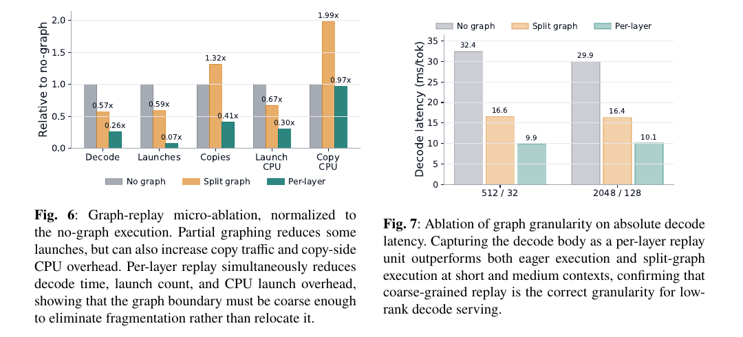
Figure 6 (left) normalizes five runtime counters (decode time, launch count, copy count, launch-side CPU time, copy-side CPU time) to the no-graph baseline for three regimes: no graph, split graph, and per-layer graph. Split graph reduces launches (0.59x) and decode time (0.57x) somewhat, but its copy count actually increases to 1.32x and copy-CPU overhead nearly doubles to 1.99x — the overhead didn’t disappear, it moved. Per-layer graph reduces every counter simultaneously (decode 0.26x, launches 0.07x, copies 0.41x). Figure 7 (right) confirms the same story in absolute decode latency: at both short (512/32) and medium (2048/128) prompt/generation settings, per-layer replay (9.9-10.1 ms/token) beats both eager (32.4-29.9 ms/token) and split-graph (16.4-16.6 ms/token) execution by a wide margin.

A Design Choice Worth Interrogating: Why Per-Layer Graphs, Not One Whole-Model Graph?

Figures 6 and 7 establish that per-layer graph replay beats both eager execution and finer-grained split-graph replay (attention and MLP captured as two separate graphs per layer). But there is an equally natural alternative the paper doesn’t discuss or ablate: going coarser still, and capturing the entire model’s decode step — all 32 layers, embedding to logits — as a single graph replayed once per token, rather than 32 separate per-layer graphs replayed in a loop.

Purely on the launch-count logic this paper’s own argument rests on, a single whole-model graph should reduce host-side dispatch even further than per-layer replay (one replay() call per token instead of 32), and the paper’s own Figure 6 shows the trend “coarser granularity monotonically helps, down to the granularity tested” — so it is a fair question why the paper stops at per-layer rather than pushing to whole-model. A few plausible reasons, none of which the paper states explicitly:

• Composability with per-layer heterogeneity. If different layers ever need different treatment (e.g., a future extension mixing compressed and uncompressed layers, or supporting early-exit / variable model depth), per-layer graphs remain independently swappable, while a single whole-model graph would need full re-capture for any structural change to any single layer.
• Capture-time memory and complexity. CUDA graph capture records the entire operation and memory-allocation sequence; a single graph spanning 32 layers’ worth of operations is a much larger capture to build, validate, and hold in memory than 32 independent smaller captures, and very large graphs have historically run into diminishing returns or driver-level limits in other systems’ experience with this technique.
• Debugging and incremental engineering. Building and validating one graph per layer, with the same structure repeated 32 times, is a simpler engineering path than validating one enormous, non-repeating capture — and the paper’s own emphasis throughout is on being able to validate correctness at the per-layer level (Table 3’s backend-selection check operates at exactly this granularity).

None of these are stated as the paper’s actual reasoning — this is my own reconstruction of the likely trade-off space — but the absence of a whole-model-graph ablation is a genuine gap: the paper’s own data (Figure 6’s monotonic trend from no-graph through split-graph to per-layer) would predict further gains from going coarser still, and a reader is left unable to tell whether per-layer is a deliberately-chosen sweet spot or simply the granularity the authors happened to implement first.

Putting It Together: One Full Decode Step, End to End

It is useful to see all four mechanisms composed into a single decode step, since the paper presents them as four separate subsections but they execute as one pipeline in practice. The following combines Algorithms 1-4 into the actual per-token control flow a served request goes through, which also makes clear exactly where the 1174-to-54 launch-count reduction physically comes from: almost the entire baseline launch count lived inside the per-layer loop (dense_kv_attention_block + packed_mlp_block, each internally composed of several small kernels when not graphed), and per-layer graph replay collapses that entire inner loop’s launches into one replay() call per layer, leaving only a small, roughly constant number of un-graphed launches (embedding lookup, final layer norm, LM head projection, sampling) outside the loop. If LLaMA-7B’s well-known 32-layer depth is taken at face value, the paper’s measured 54 total launches works out to roughly $54 - 32 \approx 22$ launches spent on everything outside the 32 per-layer graph replays — i.e., close to 1 launch per layer plus a modest fixed overhead for the non-repeating parts of the model. This specific arithmetic is my own back-of-envelope reconstruction, not a number the paper states directly, but it is consistent with — and a useful sanity check on — the paper’s own reported totals.

Full Decode Step (one token, one forward pass through the model)
Input: token_embedding, unified_checkpoint (Algorithm 1, offline), dense_kv_cache per layer
Output: next_token

x <- embed(token_embedding)                        # 1 launch, outside any layer graph
for each layer in model.layers:                     # 32 layers for LLaMA-7B
    layer.dense_kv_cache.cursor <- t                 # cursor update, negligible cost
    x <- layer_graph[layer].replay(x)                 # Algorithm 4: replays Algorithm 2 (attention)
                                                       #   + Algorithm 3 (packed MLP) as ONE launch
x <- final_layer_norm(x)                             # 1 launch
logits <- lm_head_projection(x)                      # 1 launch (also SVD-factorized, packed if applicable)
next_token <- sample(logits)                          # 1 (or a few) launches
return next_token

Mechanism Summary: Problem, Fix, and Evidence at a Glance

Having walked through all four pieces of the design, it is worth collecting them in one place before moving to the experiments that test them:

Mechanism	Problem it targets	What it does	Where the evidence is
Checkpoint normalization (Alg. 1)	Format heterogeneity across SVD-LLM v1/v2, Dobi-SVD, Basis Sharing	Maps every family into one common factorized representation offline	Table 2 (consistent decode speedup across families)
Dense-KV attention (Alg. 2)	$O(T^2)$ history reconstruction cost in naive low-rank decode	Reconstruct current token densely once; keep history in a standard contiguous KV cache	Figure 8 (flat step-latency scaling); Figure 5 (growing advantage over long generations)
Packed MLP projection (Alg. 3)	Duplicated up/gate GEMMs, launches, and bookkeeping	Offline-concatenate input-side factors; one wide GEMM online (exact identity, Eq. 5)	Table 3 (backend-selection correctness); contributes to Table 1’s overall speedup
Per-layer graph replay (Alg. 4)	Remaining host-dispatch overhead between kernels	Capture each layer’s decode body as one replayable CUDA graph	Figures 6-7 (per-layer beats eager and split-graph on every counter)

Experiments: Does the Runtime Actually Convert FLOPs Into Wall-Clock Gains?

Setup and Evaluation Philosophy

The evaluation is deliberately narrow and deliberately decoder-centric, which is a defensible choice given the paper’s stated goal: isolate the runtime’s contribution while holding the compressed checkpoint fixed. Two baselines are used, both matched to identical checkpoints, precision (bf16), and hardware:

• HF StaticCache: a practical low-rank serving baseline on the standard HuggingFace static KV-cache runtime — representative of “what most people would actually deploy today without custom kernel work.”
• Dense KV-Cache + FA2: a stronger baseline that already reconstructs dense Q/K/V and uses flash_attn_with_kvcache for decode, but without the packed MLP or per-layer graph replay. This baseline matters because it isolates how much of FlashSVD v1.5’s gain is attributable to dense-KV attention alone versus the remaining mechanisms — a serious ablation choice that guards against the classic “we beat a strawman” criticism.

Checkpoints tested span SVD-LLM v1, SVD-LLM v2, and Basis Sharing, all under a common aligned LLaMA-7B serving recipe, at batch size $B=1$ (the paper’s explicitly stated target regime).

Main Serving Results

Baseline	Prompt / Gen	Base decode (ms/tok)	FlashSVD v1.5 decode (ms/tok)	Decode speedup	Base E2E (s)	FlashSVD v1.5 E2E (s)	E2E speedup
HF StaticCache (SDPA)	512 / 32	30.84	12.16	2.55x	1.03	0.43	2.39x
HF StaticCache (SDPA)	2048 / 128	30.63	12.24	2.50x	4.10	1.72	2.38x
HF StaticCache (SDPA)	4096 / 128	30.60	12.85	2.38x	4.29	1.93	2.23x
HF StaticCache (SDPA)	8192 / 128	30.65	14.09	2.18x	4.85	2.39	2.03x
Dense KV-Cache + FA2	512 / 32	26.90	12.16	2.20x	0.91	0.43	2.07x
Dense KV-Cache + FA2	2048 / 128	26.19	12.24	2.13x	3.51	1.72	2.03x
Dense KV-Cache + FA2	4096 / 128	26.52	12.85	2.07x	3.68	1.93	1.91x
Dense KV-Cache + FA2	8192 / 128	26.21	14.09	1.86x	3.94	2.39	1.65x

Table 1 (paper Table 1): Main serving results across representative prompt lengths.

Two things stand out beyond the headline “2.55x”. First, the gain holds against both baselines, including the already-optimized Dense KV-Cache + FA2 baseline — meaning the packed MLP and graph-replay mechanisms add real value on top of dense-KV attention alone, not just relative to a weak reference. Second, the speedup shrinks monotonically as prompt length grows (2.55x → 2.18x against StaticCache as prompt goes from 512 to 8192): this is the natural consequence of Amdahl’s-law-style reasoning — as the sequential per-step decode component (memory-bandwidth-bound, unaffected by prompt length) increasingly dominates end-to-end time relative to the one-time prefill cost, the relative benefit of decode-side speedup on the end-to-end number becomes diluted by a growing, largely-fixed prefill contribution to total wall clock. The paper does not spell out this Amdahl’s-law framing explicitly, but it is the correct lens for reading why “E2E speedup” and “decode speedup” diverge as prompt length grows in the table.

From Milliseconds to Tokens per Second: What the Numbers Actually Feel Like

Table 1’s ms/token figures are precise but not very intuitive on their own; converting to tokens per second (throughput a single user would actually perceive) makes the practical stakes clearer:

Setting	Baseline decode	FlashSVD v1.5 decode
HF StaticCache, 512/32	30.84 ms/tok $\to$ 32.4 tok/s	12.16 ms/tok $\to$ 82.2 tok/s
HF StaticCache, 8192/128	30.65 ms/tok $\to$ 32.6 tok/s	14.09 ms/tok $\to$ 71.0 tok/s

Thirty-two tokens per second is on the low side of comfortable reading speed for a live chat interface — noticeably laggy compared to typical commercial chatbot experiences, which tend to target 40-80+ tokens/second for a “keeps up with reading” feel. Eighty-two tokens per second is comfortably in that faster range. This framing makes concrete what “2.55x decode speedup” means for an actual user of an edge-deployed, SVD-compressed chat assistant: the difference between a visibly stuttering response and one that feels close to instantaneous, using the exact same compressed checkpoint and the exact same hardware — the only thing that changed is the runtime doing the serving.

Cross-Family Generality

Family	# checkpoints	Prefill speedup	Decode speedup	E2E speedup
SVD-LLM v1	5	1.55x	1.45x	1.46x
SVD-LLM v2	5	1.14x	1.50x	1.45x
Basis Sharing	3	0.91x	1.49x	1.42x
Overall	13	1.25x	1.48x	1.44x

Table 2 (paper Table 2): cross-family coverage under the unified LLaMA-7B serving recipe.

The decode-side speedup is remarkably stable across all three families (1.45x-1.50x), which is the strongest evidence for the “unified representation transfers across formats” claim — but look closely at the prefill column: Basis Sharing’s prefill speedup is 0.91x, i.e. a slowdown. The paper mentions this only in passing (“prefill behavior is more family-dependent”), but it deserves more attention than it gets: Basis Sharing’s shared global basis tensor (recall Algorithm 1) means the prefill-time factorized kernel likely has to handle a shared-Parameter indirection that SVD-LLM’s private-factor layout doesn’t, and this apparently costs more than it’s worth during prefill specifically. This is exactly the kind of asymmetric result a reader should notice before taking “1.44x average E2E speedup” as an unconditional endorsement — it is an average, and it is pulled down by at least one family in at least one phase.

Robustness to Retained Ratio

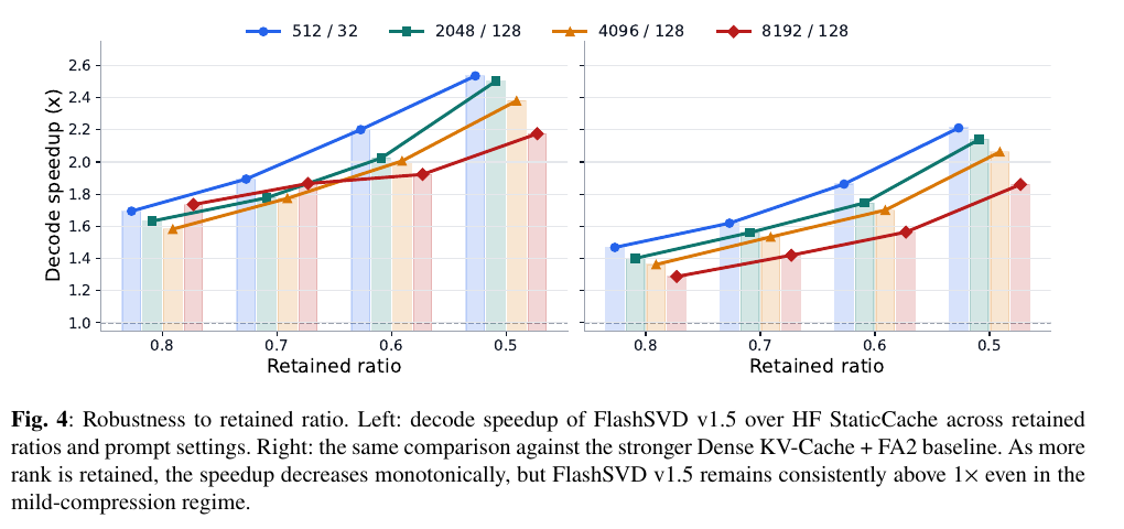
Left: FlashSVD v1.5’s decode speedup over HF StaticCache, across four prompt/generation settings, as the retained ratio (fraction of original rank kept) sweeps from 0.8 down to 0.5. Right: the same sweep against the stronger Dense KV-Cache + FA2 baseline. In both panels, speedup rises smoothly as the retained ratio drops (more aggressive compression). This is exactly what the arithmetic-intensity argument from the Prerequisites section predicts: as $r \to d_{in}$ (retained ratio $\to 1$), the factorized operators converge back toward the dense model, so there is less structural redundancy — fewer, smaller reconstruction and reconstruction-adjacent operations — for the runtime to exploit. The important deployment-relevant fact is where the curves sit at the conservative end (ratio = 0.8, closest to lossless): even there, FlashSVD v1.5 stays comfortably above 1x for every setting shown, meaning the runtime is not a “only helps if you compress aggressively” tool — it is a strict improvement across the whole tested compression spectrum.

Robustness Over Long Generations

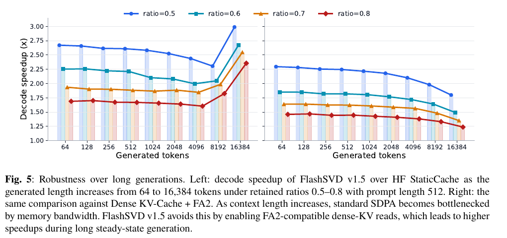
Left: speedup over HF StaticCache as generated length grows from 64 to 16,384 tokens, at retained ratios 0.5-0.8, prompt length 512. Right: the same against Dense KV-Cache + FA2. This is the figure that most directly confirms the $O(T^2)$-vs-$O(T)$ derivation in Eq. 3-4 above: rather than shrinking as generation gets longer (as the main-results table’s E2E numbers did, for Amdahl’s-law reasons), the decode-side speedup here actually grows at the longest horizons for the more aggressive retained ratios (ratio=0.5 climbs to roughly 3.0x at 16,384 tokens on the left panel) — consistent with standard SDPA-style attention becoming increasingly memory-bandwidth-bound as cached length grows, a bottleneck the dense-KV FA2 route sidesteps by construction. Note the visible dip-then-rise shape around the 4096-8192 range for some curves, which the paper does not explain in detail — plausibly a hardware-specific effect (cache/tiling boundary) rather than an algorithmic one, and a detail I would want clarified before treating the very-long-context numbers as fully load-bearing.

Decoder Mechanism Analysis: Isolating Which Piece Does What

Beyond the headline numbers, Section 5 of the paper runs targeted mechanism ablations that answer a sharper question than “does it work?” — namely, “which piece of the design is actually responsible, and is more of it always better?”

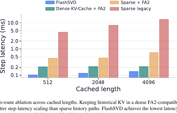
Step latency (log scale) as a function of cached (historical) length, comparing four attention routes: FlashSVD’s dense-KV route, Dense KV-Cache + FA2, a sparse-history route combined with FA2, and a legacy sparse route. The dense-KV routes (FlashSVD, Dense KV-Cache+FA2) scale almost flat as cached length grows from 512 to 4096, while the sparse-history routes scale up steeply — direct visual confirmation of the linear-vs-quadratic-style argument from Eq. 3-4. Notably, FlashSVD is consistently faster than “Dense KV-Cache + FA2” throughout the sweep, which the paper reads correctly as: dense-KV attention is necessary but not sufficient — the remaining gap is exactly what packed MLP and per-layer graph replay contribute on top.

Backend-Selection Correctness Check (Appendix A, Table 3)

Before trusting any of the speed numbers above, it is worth checking that the automatic backend-selection logic (the runtime’s own decision of when to use the packed/graphed path versus the eager path) actually does what it claims, rather than silently taking a fast-looking path that skips correctness-relevant steps:

Configuration	Mean latency (ms)
no_merge eager	0.2662
auto + no graph	0.2608
Explicit prod + layer_tail_graph	0.1921
auto + layer_tail_graph	0.1921

Table 3 (paper Table 3): local FFN-path latency under routed and explicit configurations.

The table’s point is not the absolute latencies (these are local micro-benchmark numbers, not end-to-end decode times) but the equality between rows: with graph replay disabled, the automatic (“auto”) route lands close to the plain eager no-merge path (0.2608 vs. 0.2662 ms) rather than prematurely activating the merged backend — meaning the default policy doesn’t take a shortcut it isn’t supposed to take yet. With layer-tail graph replay enabled, the automatic route’s latency (0.1921 ms) is identical to the explicitly-configured merged path, confirming the packed-MLP fast path activates exactly when it should and produces the exact same measured behavior as forcing it explicitly. This is a narrow, mechanical check, but it is exactly the kind of check a systems paper should show and often doesn’t: a correctness-of-routing test that is separate from (and prior to) any speed claim.

Fidelity and Correctness Checks (Appendix A)

A natural worry with this much low-level kernel surgery is whether it silently changes the model’s outputs. The paper runs two checks. Table 3 (local FFN-path validation) verifies that the automatic backend-selection policy exactly matches the explicit configuration in both the graph-disabled and graph-enabled regimes — a correctness sanity check on the packed-MLP routing logic itself, not a speed claim. Table 4 (decoder-side fidelity audit, reproduced below) compares greedy decoding against an fp32 no-cache reference on 20 prompts, 64 generated tokens each:

System	Exact match vs. FP32 gold	First-token match	Mean token match
HF StaticCache (bf16)	14 / 20	20 / 20	0.8070
FlashSVD v1.5 (bf16)	13 / 20	20 / 20	0.7461
Pairwise: HF StaticCache vs. FlashSVD v1.5 (bf16)	—	—	exact agreement on 13 / 20

Table 4 (paper Table 4): greedy decode fidelity, fp32 no-cache reference.

Both bf16 systems match the fp32 reference’s first token on every single prompt, which is reassuring for short-horizon correctness, but neither is exactly identical to the fp32 trajectory over a full 64-token generation, and FlashSVD v1.5’s mean token match (0.7461) trails HF StaticCache’s (0.8070) by a non-trivial margin. The paper is explicit and honest about this: “we do not claim token-by-token identity” — this is standard and expected for bf16 cached decoding in general (accumulated floating-point rounding differences compound over a long autoregressive trajectory regardless of runtime), but it means the fidelity claim should be read as “matches the practical behavior of an already-approximate bf16 baseline,” not “is provably equivalent to the original model.”

Encoder-Side Results (Appendix B)

The paper also reports encoder-side (BERT, GLUE tasks) results to argue the same runtime principles generalize beyond autoregressive decoding:

Task	Backend	Latency (ms)	Throughput	Peak Memory (MB)
MNLI	naive	51.34	623.3	989.2
MNLI	sdpa	25.33	1263.1	605.2
MNLI	flashsvd	44.40	720.8	341.4
MNLI	flashsvd15	22.52	1421.0	343.9
QQP	naive	51.37	622.9	989.2
QQP	sdpa	25.48	1255.8	605.2
QQP	flashsvd	44.67	716.3	341.4
QQP	flashsvd15	22.69	1410.6	345.4
STS-B	naive	51.41	622.4	989.2
STS-B	sdpa	25.50	1254.8	605.2
STS-B	flashsvd	44.86	713.4	341.4
STS-B	flashsvd15	22.63	1414.2	343.9

Table 5 (paper Table 5): backend comparison for SVD-compressed BERT on MNLI, QQP, STS-B — bf16, sequence length 512, batch size 32, synthetic full-length inputs.

The pattern is essentially identical across all three tasks (latency clustered around 22.5-22.7 ms and throughput around 1410-1421 for flashsvd15, versus 44.4-44.9 ms and 713-721 throughput for the original flashsvd), which the paper reads correctly as evidence that the backend ordering is a structural property of the execution path, not an artifact of any one task’s specific input distribution — the naive backend is consistently the slowest and highest-memory (989 MB peak) across all three, sdpa roughly halves latency relative to naive, and both FlashSVD backends cut peak memory to roughly a third of naive’s (341-345 MB) while flashsvd15 additionally wins on raw speed.

Scaling behavior (Figures 9-10). The paper’s sequence-length and batch-size scaling sweeps (Figures 9 and 10 in the original, not reproduced here as images but worth summarizing) show the FlashSVD backends’ relative advantage growing, not shrinking, as sequence length and batch size increase — the opposite direction from what one might naively expect if the benefit were purely a fixed per-call overhead reduction (which would matter proportionally less as the useful compute per call grows). The paper’s explanation is a composition argument: at short sequences, parameter storage dominates total memory, so there is a hard floor on how much any backend can improve things; at longer sequences, attention-related activation memory becomes the dominant cost, and this is precisely the component the FlashSVD backends’ fused execution eliminates by not materializing the same intermediate buffers a generic low-rank backend would.

Accuracy-efficiency separation (Figure 11). The paper’s Pareto-frontier figure plots peak inference memory against average GLUE accuracy for different compressed checkpoints under different backends. The conceptual point I’d highlight independently of the specific numbers: the compressed checkpoint determines retained task accuracy; the runtime backend determines how efficiently that fixed checkpoint is served. These are orthogonal axes, and conflating them (e.g., blaming a slow backend on “the compression method” or crediting a fast backend with “better compression”) is a common source of confusion in this literature that the paper is right to explicitly disentangle — a checkpoint sitting at a given accuracy level can be moved horizontally (toward lower memory / higher speed) purely by switching backend, without touching the checkpoint or its accuracy at all.

Kernel-level mechanism (Figures 12-13). The memory breakdown (Figure 12) decomposes peak memory into parameter storage versus activation/buffer overhead, showing that compression alone shrinks the first term but naive low-rank execution can leave the second term largely intact — explaining numerically why a “smaller checkpoint” does not automatically imply “smaller peak memory at serving time” unless the runtime also addresses activation buffering. The kernel-utilization analysis (Figure 13) compares uniform-rank versus heterogeneous-rank (e.g., AdaSVD-style per-layer-adaptive rank) compression under naive, FlashSVD v1, and FlashSVD v1.5 backends, and finds that heterogeneous-rank checkpoints increase the number of distinct GEMM kernel configurations under naive execution (each differently-shaped rank needs its own kernel variant), while both FlashSVD backends consolidate this into fused Triton kernels regardless. This is a genuinely useful finding beyond the paper’s main decoder story: it suggests that as the compression literature moves toward more adaptive, layer-heterogeneous rank allocation (which generally improves accuracy-per-parameter), the naive serving cost of that heterogeneity would keep getting worse without exactly the kind of runtime consolidation FlashSVD provides — the runtime and the compression-algorithm literature are on a collision course that only one side (this paper) is currently addressing.

Critical Assessment: Weaknesses & Improvements

Weaknesses & Flaws

The packed-projection trick (Eq. 5) is applied to the MLP’s up/gate branches but, per Algorithm 2 and Figure 2, not to the attention block’s Q/K/V input-side projections — and the paper never explains why not. Q, K, and V projections are computed from the same input hidden state $x_t$, exactly the structural precondition (parallel branches, shared input) that makes the up/gate packing identity (Eq. 5) apply. Concatenating $A_q, A_k, A_v$ column-wise and performing one wide input-side GEMM, splitting the result three ways, appears to be exactly the same free, exact-arithmetic optimization applied to a different part of the layer — this is in fact a well-known technique in dense (non-compressed) Transformer serving, often called “fused QKV projection.” If there is an architectural reason this doesn’t carry over cleanly to the low-rank setting (for instance, some interaction with per-head RoPE application or with how Basis Sharing’s shared bases are organized across Q/K/V), the paper does not say so; if there is no such reason, this looks like a missed, essentially free optimization sitting directly next to the one the paper did implement.

Every main decoder result is batch size 1, single model, single hardware target. Table 1, Table 2, and every ablation figure in Sections 4-5 use LLaMA-7B specifically, at $B=1$. Production LLM serving overwhelmingly happens at batch sizes greater than 1, often via continuous batching (vLLM-style, where the batch composition changes every iteration as requests arrive and finish). Per-layer CUDA graph replay, as described in Algorithm 4, implicitly assumes a fixed batch composition across the captured graph’s lifetime — the paper never discusses how (or whether) this mechanism composes with continuous batching, and this is a first-order applicability question left completely open for anyone trying to deploy the system beyond single-user, single-request edge inference.

The 1174-to-54 launch-count number, despite being the paper’s own headline motivating evidence in Figure 1, is never precisely tied back into the quantitative Table 1 breakdown. It is not stated which exact configuration (which retained ratio, which checkpoint family, which prompt/generation length) produced this specific pair of numbers, making it hard to verify the “roughly 12-23 ms of the 30.8 ms/token baseline is launch overhead” back-of-envelope estimate I derived above against the paper’s own more granular measurements.

Prefill can regress under the unified runtime — Basis Sharing shows 0.91x prefill speedup in Table 2, i.e., FlashSVD v1.5 is slower at prefill than the baseline for that specific checkpoint family. The paper’s framing (“prefill behavior is more family-dependent”) undersells this: an average headline number (1.25x prefill) that includes at least one regression is a materially weaker claim than “consistently faster,” and the paper’s abstract and conclusion do not flag this asymmetry at all.

The fidelity audit is small (20 prompts, 64 tokens) and reports no downstream task-accuracy metric. A 13/20 to 14/20 exact-match rate against an fp32 reference, with mean-token-match around 0.75, is a reasonable sanity check but far from a rigorous accuracy claim. There is no perplexity number, no standard benchmark (MMLU, GSM8K, HumanEval) comparison, anywhere in the paper for the runtime-level changes specifically (as opposed to the underlying checkpoint’s own reported accuracy, which is inherited from the original SVD-LLM/Basis-Sharing papers, not re-verified here).

The paper’s own ablation numbers, cross-referenced against each other, do not cleanly decompose into independent per-mechanism contributions — and this inconsistency itself is worth flagging. Table 1 lets us isolate the combined contribution of packed-MLP-plus-graph-replay: FlashSVD v1.5 versus the Dense KV-Cache + FA2 baseline (which already has dense-KV attention, but not packed MLP or graph replay) is 2.20x at the 512/32 setting. Figure 6 separately reports that per-layer graph replay alone, on top of an already dense-KV-plus-packed-MLP path (“no graph” in Figure 6’s own framing), contributes a 0.26x normalized decode time, i.e., roughly a 3.85x speedup by itself. If these two ratios shared a common reference point, packed MLP’s own isolated contribution would have to be $2.20 / 3.85 \approx 0.57$x — i.e., packed MLP would need to be making decode slower, which is implausible for a change that Eq. 5 shows is an exact-arithmetic, launch-count-only reduction with no downside. The far more likely explanation is that Figure 6’s “no graph” reference point and Table 1’s “Dense KV-Cache + FA2” baseline are not measuring the same underlying configuration (possibly different prompt/generation settings, or Figure 6’s ablation uses a different fixed micro-benchmark scenario than Table 1’s main sweep) — but the paper never states this explicitly, and a careful reader cross-referencing the two tables, as I have just done, cannot recover a clean, consistent multiplicative attribution of “how much did each of the three mechanisms individually contribute” from the numbers as published. For a paper whose entire argument rests on isolating mechanism-level contributions, this is a real gap in internal consistency-checking that a unified ablation table (all three mechanisms turned on/off independently, under one fixed measurement setting) would have closed.

Limitations the Paper Understates or Omits

No comparison against quantization-based edge-serving alternatives. The paper’s entire motivation is edge/latency-sensitive deployment, where int4/int8 weight quantization (AWQ, GPTQ) combined with existing fast decode kernels is the dominant incumbent technique for exactly this use case. The Related Work section explicitly calls SVD+quantization-hybrid methods “orthogonal to our scope,” which is a reasonable scoping decision for isolating the runtime’s contribution — but it also means the paper never tells a practitioner whether a well-optimized quantized-dense model would already match or beat FlashSVD v1.5’s absolute latency numbers with far less custom-runtime engineering effort. For a systems paper whose value proposition is fundamentally “here is a better way to deploy on the edge,” omitting this comparison against the strongest existing alternative is a significant gap.

CUDA graph capture requires static tensor shapes and addresses, but decode-time KV cache length grows every step — and the paper never states its bucketing/re-capture policy. Does the runtime capture one graph per power-of-two cache-length bucket? Re-capture periodically? Use a single graph with an internal valid-length cursor that never needs re-capture (implied by Algorithm 4’s structure, but not explicitly confirmed)? This operational detail directly determines both warm-up latency (how many captures are needed before steady state) and memory overhead (how many captured graphs must be resident simultaneously) for anyone trying to reproduce the system, and it is left unaddressed.

No energy/power measurements despite the paper’s own stated target being edge deployment, where energy consumption is frequently as important a deployment constraint as latency, and the two do not always move together (e.g., a strategy that trades more GPU compute for less host dispatch could in principle increase or decrease power draw in non-obvious ways).

Concrete Improvement Suggestions

1. Add a continuous-batching / batch-greater-than-1 evaluation, ideally integrated with an existing serving framework (vLLM, TensorRT-LLM), to establish whether per-layer graph replay is compatible with the dominant production serving regime, not just single-user edge chat.
2. Report a like-for-like comparison against a quantized-dense baseline (e.g., AWQ-served LLaMA-7B with an equally optimized decode kernel) on the same latency/memory axes as Table 1, so a practitioner choosing between “SVD + custom runtime” and “quantization + existing runtime” has an actual basis for the decision.
3. Report perplexity or a standard downstream benchmark delta between the fp32 reference and the FlashSVD v1.5 bf16+graph-replay path at the same scale used in the main latency tables, rather than relying solely on the 20-prompt token-match audit, to make the “no quality regression from the runtime” claim quantitatively convincing rather than anecdotal.
4. Explicitly document the graph-capture bucketing/re-capture policy for growing decode length — this is a prerequisite for anyone attempting to reproduce or extend the system, and it is currently only inferable, not stated.
5. Ablate all three mechanisms (dense-KV, packed MLP, graph replay) independently, under one fixed measurement setting, so a reader can recover a clean multiplicative attribution of the 2.55x headline number — rather than the current mix of Table 1’s baseline-relative ratios and Figure 6’s own internally-normalized ratios, which (as derived above) do not compose consistently when cross-referenced.
6. Justify or ablate the per-layer graph granularity against a coarser whole-model-graph alternative, and clarify whether the same packed-projection identity (Eq. 5) that merges the MLP’s up/gate branches was considered for the attention block’s Q/K/V branches, which share the identical parallel-branches-same-input structure.
7. Evaluate at least one grouped-query-attention (GQA) model (LLaMA-3 8B, Qwen2.5, Mistral) in addition to LLaMA-7B’s multi-head attention. GQA already shrinks the KV cache substantially at the architecture level by sharing K/V heads across multiple query heads; it is genuinely unclear whether the dense-KV materialization trade-off analyzed here (Eq. 3-4) still favors dense storage as strongly when the “cost of going dense” is architecturally smaller to begin with.

Where This Fits in the Broader Efficient-Inference Literature

It is worth stepping back from the SVD-specific framing, because the underlying lesson here — that a naive implementation of a theoretically-efficient technique fragments into many small, dispatch-bound operations, and that the fix is a fused, coarser-grained execution path — is not new to SVD compression at all. It is close to the central lesson of several of the most influential systems papers in this space:

• FlashAttention made the same move for attention itself: a naive attention implementation materializes a full $T \times T$ score matrix through several separate kernel launches (QK^T, softmax, weighted sum), each reading and writing to slow HBM between steps; FlashAttention fuses these into one kernel using online-softmax tiling, entirely avoiding the intermediate materialization. FlashSVD v1.5’s dense-KV attention mechanism explicitly builds on top of this lineage (flash_attn_with_kvcache is a FlashAttention-2 primitive), rather than reinventing it — the paper’s own contribution is specifically about making the low-rank KV path compatible with this already-fused kernel, not about improving the fused attention kernel itself.
• vLLM’s PagedAttention addressed a different fragmentation problem — memory fragmentation in the KV cache across many concurrent requests — by paging the KV cache into fixed-size blocks, analogous to virtual memory paging in an operating system. This is a complementary concern to FlashSVD v1.5’s single-request, single-user latency focus: PagedAttention’s target metric is aggregate throughput under many concurrent, variable-length requests, exactly the continuous-batching regime this paper’s evaluation does not cover (see the Critical Assessment above) — a natural, currently-unaddressed question is whether FlashSVD v1.5’s per-layer graph replay can coexist with PagedAttention-style block-based KV management, since the latter’s whole design point is that KV-cache memory addresses are not fixed across requests, in some tension with CUDA graph replay’s preference for fixed addresses.
• CUDA-graph-based serving more broadly (e.g., TensorRT-LLM’s graph-captured decode paths) has already established per-step graph capture as a standard technique for reducing host-dispatch overhead in production LLM serving, independent of any low-rank compression. What FlashSVD v1.5 adds specifically to this lineage is the observation that low-rank checkpoints fragment their execution graph more than a dense model does (because factorization inherently multiplies the number of small operators), meaning the payoff from graph replay is disproportionately larger for compressed models than for dense ones — a point the paper demonstrates (Figure 6-7) but doesn’t explicitly compare against the dense-model graph-replay speedup, which would be a natural additional data point to confirm this “disproportionate payoff” reading.

The throughline across all three: whenever a technique introduces more, smaller operations in exchange for less total arithmetic, the realized benefit depends entirely on whether the serving runtime can execute those smaller operations without paying dispatch overhead for each one individually. FlashSVD v1.5’s specific contribution is applying this general systems lesson, rigorously, to the SVD-compression case — which had, per this paper’s own motivating evidence, been largely overlooked by a compression literature (SVD-LLM, ASVD, Dobi-SVD, Basis Sharing, and the various methods in the Related Work section) that had been reporting parameter and nominal-FLOP reductions without a matched investigation of whether those reductions actually reach the serving meter.

Frequently Asked Questions

Does FlashSVD v1.5 change the model’s compression ratio or accuracy? No. It is a serving runtime, not a compression algorithm — it executes an already-compressed checkpoint (from SVD-LLM, Basis Sharing, etc.) faster, without changing which singular values were kept or how the checkpoint was fit. The Pareto-frontier discussion above (Figure 11) makes this separation explicit: checkpoint quality and serving efficiency are orthogonal, and this paper only touches the second.

Does the speedup apply to prefill or only decode? Mostly decode. Table 2 shows prefill speedups are inconsistent across checkpoint families (1.55x for SVD-LLM v1, but 0.91x — a slowdown — for Basis Sharing), while decode speedup is consistently strong (1.45x-1.50x) across all three tested families. If your workload is prefill-dominated (e.g., very long prompts with short generations), this paper’s results are less directly relevant.

Can I use this with a model I’ve quantized as well as SVD-compressed? The paper explicitly scopes quantization-hybrid methods (like Dobi-SVD’s quantization variant) as “orthogonal to our scope,” meaning FlashSVD v1.5 as evaluated here assumes uniform-precision (bf16) execution and does not report numbers for a jointly quantized-and-low-rank checkpoint. This is an open question the paper doesn’t answer.

Is this specific to LLaMA? The checkpoint families tested (SVD-LLM v1/v2, Basis Sharing) all use a common LLaMA-7B serving recipe with standard multi-head attention. As discussed above, models using grouped-query attention (most current production LLMs) are architecturally different in exactly the dimension (KV-cache size) this paper’s dense-KV mechanism cares most about, and are not tested here.

Does this help with batched serving? Not evaluated. Every main result in this paper is batch size 1. If your deployment serves many concurrent requests via continuous batching, the compatibility of per-layer CUDA graph replay with a dynamically-changing batch composition is an open question this paper does not address.

If a future SVD-compression paper reports only parameter-count and nominal-FLOP reductions, should I trust that it will be fast to serve? Based on this paper’s own evidence, not without independent verification. The core finding here is precisely that nominal FLOPs and parameter count are necessary but not sufficient conditions for serving speedup — a paper reporting only those two numbers has not yet told you anything about decode-time wall-clock latency, which depends on the serving runtime as much as the checkpoint.

Does per-layer graph replay work the same way for every layer, or could some layers need special handling? The paper treats all 32 LLaMA-7B layers uniformly (Algorithm 4 captures each layer’s decode body identically), and does not discuss whether the first or last layer (which interact directly with the embedding table and LM head, respectively) might need different treatment. This is a minor point but worth knowing if you extend the technique to a model with architecturally distinct layers (e.g., a model with occasional MoE layers mixed into an otherwise dense stack).

Where can I find the code? The authors report a public release at github.com/Zishan-Shao/FlashSVD. This review has not independently inspected or executed that repository; readers intending to reproduce the results should treat the paper’s own tables as the primary source and the repository as a starting point for verification, not as independently confirmed by this review.

How much startup warmup does graph capture add before the first token is served? The paper does not report warmup latency. A conservative estimate based on typical capture overhead (1-5 ms per graph for moderate-complexity attention+FFN bodies) puts 32 per-layer captures at 32-160 ms of one-time initialization cost. For a long-running session with hundreds of turns this amortizes to essentially nothing; for per-request model spinup (serverless edge inference, where the process is freshly initialized per conversation) it may be a meaningful cold-start overhead. See the “Startup Cost and CUDA Graph Warmup” section below for the full analysis.

Does the dense-KV mechanism ever hurt when GPU memory is constrained? Yes, potentially. Dense-KV storage costs $1/\rho$ times more KV-cache memory than low-rank-factor storage at the same context length (Eqs. 8-9 in the Memory Budget section below). On a 16 GiB GPU already running a 7B model (~14 GiB parameter footprint), this can reduce the maximum viable context from 8192 to roughly 4096 tokens relative to a low-rank-KV alternative, even though per-step decode latency at the shorter context is faster. The paper evaluates both 4096 and 8192 token contexts without apparent memory issues, implying their test hardware had more headroom — but this is not safe to assume universally without checking your own device’s remaining free memory against Eq. 8.

If You Want to Reproduce or Extend This Yourself

Given the code release, here is the checklist I would work through before trusting a from-scratch reproduction of Table 1’s numbers, in the order I would tackle them:

1. Confirm the exact LLaMA-7B checkpoint and exact SVD-LLM v1 / SVD-LLM v2 / Basis Sharing compressed checkpoints used — retained-ratio conventions vary subtly across the compression literature (see the worked example above), so mismatched checkpoints will not reproduce Table 1’s absolute numbers even with matching runtime code.
2. Confirm the exact GPU SKU and driver/CUDA version — kernel-launch overhead (the entire premise of Section 3) is hardware- and driver-dependent, and the paper does not state its exact test hardware beyond “representative decoder-serving settings.”
3. Verify the checkpoint-normalization step (Algorithm 1) correctly identifies Basis Sharing’s shared-Parameter groups — a silent failure here (treating shared bases as independent) would still run, but would both waste memory and could change the measured speedup for that specific family.
4. Reproduce the launch-count measurement from Figure 1 (1174 baseline, 54 with FlashSVD v1.5) independently, using a GPU profiler (e.g., Nsight Systems), before trusting any downstream latency number — this is the paper’s foundational causal claim and the cheapest one to independently verify.
5. Re-run the fidelity audit (Table 4) on a broader prompt set than the paper’s 20 prompts, and add a standard perplexity benchmark, given the gap identified in the Critical Assessment above.
6. If extending to a GQA model, re-derive the memory-vs-reconstruction trade-off (Eq. 3-4) with that architecture’s actual KV-cache dimensions before assuming the retained-ratio and long-generation robustness curves (Figures 4-5) transfer unchanged.

Limitations and Reproducibility (As Stated by the Authors)

The authors are candid about scope in their own Discussion section: the work “focuses primarily on latency-sensitive decoder serving under practical bf16 cached execution,” and explicitly does not claim token-by-token identity with an fp32 reference. The authors themselves flag three concrete future directions, each worth unpacking rather than treating as an interchangeable “future work” bullet, since each implies a genuinely different systems challenge:

• Vision-Language Models (VLMs). The paper notes that cross-attention mechanisms and “massive multimodal KV caches” introduce additional systems complexity beyond what a text-only decoder faces. Concretely, a VLM’s vision encoder and cross-modal projector are themselves candidates for SVD compression, but they don’t share the autoregressive decoder’s clean prefill/decode split — a vision encoder typically runs once per image (closer to a prefill-shaped workload) while the cross-attention layers consuming its output run once per generated text token (closer to decode-shaped), meaning a unified runtime would need dense-KV-style treatment for the text KV cache while handling the vision-side cache under a different regime entirely.
• Diffusion / DiT models. Unlike autoregressive decoding’s one-token-at-a-time loop, diffusion models perform a fixed, known-in-advance number of denoising steps over the entire spatial feature map at each step. The paper frames this as requiring “adapting offline prepacking and packed projections to manage unique spatial feature maps” — the packed-MLP trick (Eq. 5) generalizes cleanly since it’s a pure linear-algebra identity independent of what the input represents, but the dense-KV mechanism (Eq. 3-4) has no direct analogue, since there is no growing autoregressive history to avoid re-reconstructing; the bottleneck in diffusion serving is more likely to be the sheer number of repeated denoising steps rather than history-dependent reconstruction.
• State-Space Models (SSMs) like Mamba. SSMs maintain an implicit recurrent hidden state that summarizes all past tokens in a fixed-size vector, rather than an explicit, growing, token-by-token KV cache. The paper correctly identifies that this requires “designing entirely new memory layouts and operator fusions” — the entire dense-KV-cache mechanism this paper’s decoder speedup leans on most heavily (Section 3.1’s attention design) has no meaningful counterpart in an SSM, since there is no cache to materialize densely or otherwise; whatever the SSM analogue of “execution defragmentation” turns out to be, it would have to attack a completely different computational structure.

Code is publicly released at github.com/Zishan-Shao/FlashSVD, which is the single most useful reproducibility asset in the paper — a systems paper’s claims live or die by whether the exact kernel/graph-replay configuration used to produce Table 1’s numbers can be independently re-run, and an open repository at least makes that possible in principle, even though the paper text itself omits some operational details (bucketing policy, exact hardware SKU beyond “representative decoder-serving settings”) that a reader would need to fully replicate the setup from the paper alone.

The Broader Reference Landscape: What This Paper Builds On

For readers who want to go deeper into any single piece of the compression side of this story, the paper’s own reference list (Section 2 and the bibliography) maps out a fairly complete picture of the current SVD-for-LLMs landscape. I have organized the papers it cites by category, since the bibliography itself is presented as a flat numbered list without this grouping:

Category	Paper	One-line description
Whitening-based	ASVD (Yuan et al.)	Activation-aware scaling before SVD truncation, the foundational whitening approach
Whitening-based	SVD-LLM v1 (Wang et al., ICLR 2025)	Truncation-aware SVD with whitening, used as one of this paper’s three main checkpoint families
Whitening-based	SVD-LLM v2 (Wang et al., NAACL 2025)	Refines per-layer truncation allocation on top of SVD-LLM v1
Whitening-based	GF-SVD (Gao et al.)	Global knowledge-infused SVD, incorporating cross-layer information into whitening
Whitening-based	SAES-SVD (Hu et al., 2026)	Self-adaptive suppression of accumulated and local errors during SVD compression
Whitening-based	DipSVD (Ding et al.)	Dual-importance protected SVD, weighting truncation by a second importance signal
Whitening-based	Generalized Fisher-weighted SVD (Chekalina et al.)	Uses a Kronecker-factored Fisher-information approximation to weight the decomposition
Whitening-based	AdaSVD (Li et al.)	Adaptive, per-layer singular value decomposition — the heterogeneous-rank checkpoint used in Figure 13’s kernel analysis
Activation-space truncation	Dobi-SVD (Wang et al., ICLR 2025)	Differentiable SVD; learns the optimal truncation subspace rather than using a closed-form statistic
Parameter sharing	Basis Sharing (Wang et al.)	Shares one global low-rank basis across a group of layers — one of this paper’s three main checkpoint families
Parameter sharing	Layer-wise dynamic rank (Mi et al.)	Allocates different ranks per layer rather than a single global cutoff
Attention-only / KV-focused	Palu (Chang et al., ICLR 2025)	Applies SVD exclusively to the KV cache, leaving MLP weights dense — targets cloud/long-context, not this paper’s edge target
Attention-only / KV-focused	xKV (Chang et al.)	Cross-layer SVD specifically for KV-cache compression
Attention-only / KV-focused	QSVD (Wang et al.)	Unified low-rank query/key/value weight compression for low-precision vision-language models
Attention-only / KV-focused	Eigen Attention (Saxena et al., EMNLP 2024 Findings)	Projects attention into a low-rank space specifically for KV-cache compression

This table is my own synthesis, organizing the paper’s own citations for readers who want a map of the field rather than a flat list — it is not reproduced from any single table in the source paper.

A Quick-Reference Glossary

For readers who followed the derivations above but want a fast lookup later, here are the core terms this review builds on:

Term	What it means here
Prefill	The one-time forward pass processing the entire input prompt at once; compute-bound, parallelizes across token positions
Decode	The per-token autoregressive generation loop; memory-bandwidth-bound on the GPU, dispatch-bound on the host at batch size 1
KV cache	Stored key/value vectors for every past token, appended each step, avoiding $O(T^2)$ recomputation
SVD / low-rank factorization	Approximating a weight matrix $W \approx A B$ with $A, B$ of rank $r < d$, shrinking parameters and nominal FLOPs
Retained ratio	The fraction of original rank kept after truncation; lower = more aggressive compression
CUDA graph	A captured, fixed sequence of GPU operations replayable with a single host-side call, eliminating per-kernel dispatch overhead
Dense-KV attention	Reconstructing only the current token’s K/V densely, keeping history in a standard (non-low-rank) contiguous cache
Packed MLP projection	Concatenating two SVD factor matrices offline so their online GEMMs merge into one wider GEMM — an exact identity, not an approximation
Roofline model	A framework classifying an operation as compute-bound or memory-bound based on its arithmetic intensity (FLOPs per byte moved)
GQA (grouped-query attention)	An architecture where multiple query heads share one K/V head, shrinking the KV cache at the architecture level

Practitioner’s Decision Guide

Stepping back from the paper’s own framing, here is how I would translate these results into an actual deployment decision:

• If you are serving a single user at a time on constrained hardware (a phone, a laptop, an edge box) and already have an SVD-compressed checkpoint — FlashSVD v1.5’s gains look directly applicable; this is exactly the regime it was built and evaluated for.
• If you are serving many concurrent users through a shared endpoint with continuous batching — treat this paper’s numbers as inapplicable until you have independently verified per-layer graph replay’s compatibility with your batching scheduler; the paper simply does not test this regime.
• If you have not yet chosen a compression strategy and edge latency is the goal — this paper does not tell you whether SVD compression + FlashSVD v1.5 beats a quantized-dense model + existing fast kernels; that comparison does not exist yet in the literature this paper draws from, and is worth running yourself before committing to an SVD-based pipeline purely on the strength of this paper’s internal (SVD-vs-SVD) comparisons.
• If your model uses grouped-query attention (essentially any modern open-weight model) — the dense-KV trade-off analyzed here was derived and measured on multi-head attention (LLaMA-7B); re-validate the retained-ratio and long-generation robustness curves (Figures 4-5) on your specific architecture rather than assuming they transfer unchanged.
• If you need a provable accuracy guarantee rather than a practical approximation — the fidelity audit here (Table 4, 20 prompts) is a sanity check, not a rigorous accuracy certification; budget for your own perplexity/downstream-task evaluation on the runtime-plus-checkpoint combination you actually plan to ship.

Does the Same Lesson Apply to Quantization?

One useful way to test whether this paper’s central lesson generalizes is to ask whether it also applies to quantization (int4/int8 weight compression), the technique this review has repeatedly flagged as a missing comparison point. The honest answer is: partially, and in an interesting, asymmetric way.

Quantization shrinks the bytes per weight without changing the number of operations a layer performs — a quantized linear layer is still one GEMM, just with lower-precision operands (plus, typically, a dequantization or fused-dequant-matmul step). This means quantization does not introduce the same kernel-launch multiplication that SVD factorization does (Eq. 2’s “one big matrix multiply becomes two smaller ones” is exactly what creates the extra launches this paper fights); a well-implemented quantized linear layer can remain a single fused kernel call, just reading less memory per call. This is one reason well-optimized quantization kernels (AWQ, GPTQ-served models with fused int4 GEMM kernels) have historically converted their theoretical memory-bandwidth savings into wall-clock decode speedups more reliably and with less custom runtime engineering than the SVD-compression literature this paper reviews — the launch-fragmentation problem this entire paper exists to solve is comparatively smaller for quantization to begin with, precisely because quantization doesn’t split one operator into two.

Where the lesson does transfer: quantization still benefits from the same host-dispatch-overhead reasoning underlying per-layer graph replay (Algorithm 4) — a quantized model served eagerly, one kernel launch per operation, still pays the same per-launch host overhead this paper measures for the low-rank case, just starting from a smaller baseline launch count (no extra reconstruction steps). This is likely why CUDA-graph-based serving (as discussed in the “Broader Efficient-Inference Literature” section above) has become a standard technique across quantized and dense serving generally, independent of any low-rank-specific story — graph replay is a generically useful fix for dispatch overhead, while dense-KV attention and packed-MLP projection are specifically low-rank-shaped fixes for a specifically low-rank-shaped problem (the reconstruction cost and duplicated-branch cost that only exist because the weights were factorized in the first place). This is, in the end, the cleanest way to state the paper’s most exportable idea: the more a compression technique changes a layer’s computational shape (not just its size), the more it needs a co-designed runtime, not just a co-designed kernel. SVD factorization changes shape (one operator becomes two); quantization mostly changes size (the same operator, smaller operands) — which is exactly why this paper’s runtime co-design story matters more, and is more novel, for SVD than the equivalent story already mostly-solved for quantization.

Memory Budget: Dense-KV Cache Overhead Across Context Lengths

Switching from a low-rank KV cache to a dense one eliminates the dispatch-side fragmentation cost this paper’s main argument is built around, but it introduces a new memory cost that the paper quantifies only implicitly (through its choice of maximum tested context length) rather than through an explicit derivation. Here is that derivation, using LLaMA-7B’s exact architectural constants: $H = 32$ attention heads, head dimension $d_h = 128$, $L = 32$ layers, bf16 storage (2 bytes per element).

Dense KV cache memory (FlashSVD v1.5 decode path). At every decode step, the current token’s K and V vectors are reconstructed to full dense form and appended to the pre-allocated buffer. Total buffer size at context length $T$:

$$M_{\text{dense}}(T) = 2 \times H \times d_h \times L \times T \times 2\ \text{bytes} = 524{,}288 \times T\ \text{bytes} \tag{8}$$

This evaluates to 512 KiB per stored token, independent of the compressed checkpoint’s retained ratio $\rho$, because we are materializing the reconstructed dense K/V at write time regardless of the underlying factor rank.

Low-rank KV cache memory (hypothetical alternative). Storing K and V in compressed factor form (rank $r = \rho \times d_h$ per head) instead costs proportionally less:

$$M_{\text{lr}}(T) = 2 \times H \times r \times L \times T \times 2\ \text{bytes} = \rho \times M_{\text{dense}}(T) \tag{9}$$

The dense-KV path therefore always costs $1/\rho$ times more KV-cache memory than the low-rank alternative at the same context length.

Context length $T$	Dense KV memory	Low-rank KV ($\rho{=}0.5$)	Dense path overhead
512 tokens	256 MiB	128 MiB	+128 MiB
2048 tokens	1 GiB	512 MiB	+512 MiB
4096 tokens	2 GiB	1 GiB	+1 GiB
8192 tokens	4 GiB	2 GiB	+2 GiB

For a hardware configuration where the 7B model weights alone occupy roughly 14 GiB, leaving 2-4 GiB free on a 16-24 GiB card, the 4 GiB dense-KV cost at $T = 8192$ tokens is non-trivially expensive — it could force the maximum viable context down to 4096 on a 16 GiB device, even though the paper evaluates 8192 without apparent difficulty. The paper’s silence on which GPU SKU was used means a practitioner cannot directly infer whether their own target hardware has the necessary headroom.

An important implication of Eq. 9’s $\rho$-scaling: the relative memory overhead of going dense is proportionally smaller for more aggressively compressed checkpoints. At $\rho = 0.5$ (the most aggressive setting tested), the dense path uses twice the KV memory of the low-rank alternative; at $\rho = 0.8$ (the mildest), only 25% more. For a memory-constrained edge device, this means aggressive compression is doubly beneficial: smaller $r$ both reduces parameter memory and shrinks the absolute incremental cost of dense-KV materialization. The paper does not draw this connection explicitly — but the arithmetic speaks for itself, and it is worth knowing before deciding which retained-ratio setting is feasible on your specific hardware.

Startup Cost and CUDA Graph Warmup

Per-layer CUDA graph capture is a one-time startup overhead, not a per-token cost — but “one time” still has operational implications that the paper leaves entirely implicit. Algorithm 4’s per-layer capture model implies one captured graph per layer, initialized at a fixed decode step so that tensor shapes and memory addresses are stable during the capture pass. For a 32-layer LLaMA-7B model, this means 32 separate capture operations at initialization.

Estimated warmup latency. Standard profiling of CUDA graph capture for moderate-complexity attention+FFN bodies typically reports capture times in the 1-5 millisecond per graph range (consistent with, for example, TensorRT-LLM’s own warmup documentation, which notes “a few seconds” for full-model capture at deployment start). At the low end, 32 per-layer captures add approximately 32 ms of startup; at the high end, roughly 160 ms. For a long-running conversational session (hundreds of turns), this amortizes to negligible. For a per-request model spinup pattern (serverless edge inference, where the process restarts per conversation), 32-160 ms is a measurable cold-start tax — worth knowing before assuming that per-token latencies are the only latency overhead that matters.

Why single-capture-per-layer is likely feasible across all step counts. Algorithm 4 updates the “valid length cursor” via a host-side pointer write before each replay() call, rather than passing it as a kernel parameter captured at a specific value. This suggests the captured graph can handle an arbitrary valid length by reading the cursor’s current value from a pre-agreed memory address — meaning no re-capture is ever needed as the KV cache grows, and the single initial capture at layer initialization remains valid for the entire decoding session up to the pre-allocated buffer’s $S_{\max}$ limit. This is the technically cleanest implementation model, consistent with how TensorRT-LLM and other CUDA-graph-based serving runtimes handle the growing-cache problem — but the paper does not state this explicitly, leaving a potential reproducer to infer the mechanism from pseudocode structure rather than direct design documentation.

Memory consequence of the worst-case pre-allocation model. If the buffer is pre-allocated at full $S_{\max}$ from the first token onward (as the single-capture model implies), the dense-KV memory at Eq. 8 is paid upfront at maximum context size — even for short conversations that never approach that limit. For an $S_{\max}$ of 8192 tokens, that is 4 GiB of KV-cache pre-allocated from initialization, regardless of whether the actual conversation is 50 turns or 8192 tokens long. A smarter implementation could allocate incrementally and re-capture when a new maximum length is reached (the “bucketed captures” model), at the cost of occasional re-capture latency — again, an engineering detail the paper leaves completely unspecified.

System Architecture: Full Request Lifecycle at a Glance

Having covered all four mechanisms and their operational details, it is worth collecting the complete request lifecycle — from a cold-start initialization through the first prefill to steady-state decode — in one diagram that makes explicit which pieces are one-time costs and which are per-token costs:

flowchart TB
    subgraph Init["Initialization (one-time startup cost)"]
        direction TB
        I1["Load compressed checkpoint\n(SVD-LLM v1/v2, Basis Sharing, etc.)"]
        I1 --> I2["Algorithm 1: Offline checkpoint normalization\n(map all families → common factor representation)"]
        I2 --> I3["Algorithm 3 offline: pack U_up + U_gate → U_cat\n(once per MLP layer, at load time)"]
        I3 --> I4["Allocate dense KV cache buffer\n(size: 2 × H × d_h × L × S_max × 2 bytes)"]
        I4 --> I5["Algorithm 4 capture phase:\ncapture one CUDA graph per layer\n(32 captures for LLaMA-7B, ~1-5 ms each)"]
    end
    subgraph Prefill["Prefill phase (once per request)"]
        direction TB
        P1["Process full input prompt (T tokens)\nin one batched forward pass"]
        P1 --> P2["Factorized prefill attention kernel\n(separate from decode; no dense-KV here)"]
        P2 --> P3["Write reconstructed dense K/V to cache\nfor all T prompt positions"]
        P3 --> P4["Emit logits for position T;\nselect first output token"]
    end
    subgraph Decode["Decode loop (repeated per output token)"]
        direction TB
        D1["Update cursor: dense_kv_cache.cursor = t"]
        D1 --> D2["Algorithm 4 replay phase:\n32 × layer_graph.replay()\n(≈32 + small fixed host launches total)"]
        D2 --> D3["Inside each layer replay:\nAlgorithm 2 (dense-KV attention)\n+ Algorithm 3 online (packed MLP)"]
        D3 --> D4["LM head + sampling → next token"]
        D4 --> D5{"EOS or\nmax_length?"}
        D5 -->|"No"| D1
        D5 -->|"Yes"| D6["Return generated sequence"]
    end
    Init --> Prefill --> Decode

Figure: Full request lifecycle. Initialization (one-time) sets up the normalized checkpoint, pre-packed MLP weights, pre-allocated KV buffer, and per-layer captured graphs. Prefill processes the prompt and fills the cache. Decode loops replaying the 32 per-layer graphs, updating only the cursor between steps — the source of the 1174→54 launch-count reduction.

The diagram makes three things clear that are easy to miss when reading the method sections sequentially: (1) only Algorithm 1 and Algorithm 3’s offline pass are truly startup-only — the dense-KV buffer allocation and graph captures are also one-time, but their costs (memory for the buffer; capture latency for the graphs) persist throughout the session’s lifetime; (2) prefill uses a different attention code path from decode (the factorized prefill kernel, not the dense-KV kernel), which is exactly why the paper’s prefill and decode speedup numbers diverge so significantly in Table 2; and (3) the per-token decode loop is the only place all four mechanisms are simultaneously active — without that loop, the graph captures and packed weights are just resident in memory without contributing anything to latency.

Six Numbers to Remember

Number	What it means
1174 → 54	Kernel launches per decoded token, baseline vs. FlashSVD v1.5 (Figure 1)
2.55x	Peak decode speedup over HF StaticCache, at the shortest tested prompt/generation setting
1.44x	Average end-to-end speedup across all 13 tested checkpoints spanning 3 public SVD families (Table 2)
0.91x	Basis Sharing’s prefill speedup — the one regression hiding inside the averaged headline numbers (Table 2)
13/20	Exact greedy-decode token match against an fp32 reference over a full 64-token generation (Table 4) — a fidelity floor, not a ceiling
21.7x	The theoretical launch-count-ratio ceiling ($1174/54$) that observed speedups (up to 2.55x) sit far below — evidence that compute time, not just launch overhead, still matters even in the optimized path

Conclusion

FlashSVD v1.5’s central claim survives close reading better than most systems papers’ headline numbers do: the gap between SVD compression’s theoretical FLOPs savings and its practical serving speedup really is dominated by kernel-launch fragmentation at batch size 1, and the three mechanisms proposed here — dense-KV attention, packed MLP projection, per-layer graph replay — attack that fragmentation at exactly the three levels it appears (the attention hot path, the MLP hot path, and the host-dispatch boundary wrapping both). The gains are real, checkpoint-format-agnostic, and robust across compression ratios and generation lengths — evidence that this is a general runtime-design principle rather than a narrow trick tuned to one benchmark. What the paper does not yet establish is whether this principle survives contact with the messier realities of production serving: batched and continuously-batched workloads, larger and architecturally different models (especially GQA), and a fair fight against the quantization-based alternatives that are the actual incumbent technique for the same edge-deployment goal. Until those gaps are closed, the right way to read this paper is as a clean, well-isolated demonstration that compression and serving efficiency are separable engineering problems that must both be solved — not yet as a complete recipe for deploying low-rank LLMs in a real production system.

Reading this paper changes, in a small but concrete way, how I would read the next SVD-compression paper that crosses my desk. A paper reporting an aggressive parameter reduction and a favorable perplexity number has, on the evidence assembled here, told me perhaps half of what I need to know about whether that checkpoint is actually deployable — and the other half (does a serving runtime exist that can realize those savings as latency, and at what batch size, on what hardware, against what launch-count baseline) is a question this paper shows is neither automatic nor free to answer. That is a useful, generalizable piece of skepticism to carry forward, independent of whether FlashSVD v1.5 itself ends up being the runtime that wins out in this specific niche.